©2018 The Authors Journal of the Royal Statistical Society: Series C (Applied Statistics) Published by John Wiley & Sons Ltd on behalf of the Royal Statistical Society.
This is an open access article under the terms of the Creative Commons Attribution License, which permits use, dis-tribution and reproduction in any medium, provided the original work is properly cited.
0035–9254/19/68029 68,Part1,pp.29–49
Projecting UK mortality by using Bayesian
generalized additive models
Jason Hilton, Erengul Dodd, Jonathan J. Forster and Peter W. F. Smith
University of Southampton, UK
[Received January 2018]
Summary.Forecasts of mortality provide vital information about future populations, with impli-cations for pension and healthcare policy as well as for decisions made by private companies about life insurance and annuity pricing. The paper presents a Bayesian approach to the fore-casting of mortality that jointly estimates a generalized additive model (GAM) for mortality for the majority of the age range and a parametric model for older ages where the data are sparser. The GAM allows smooth components to be estimated for age, cohort and age-specific improve-ment rates, together with a non-smoothed period effect. Forecasts for the UK are produced by using data from the human mortality database spanning the period 1961–2013. A metric that approximates predictive accuracy is used to estimate weights for the ‘stacking’ of forecasts from models with different points of transition between the GAM and parametric elements. Mortality for males and females is estimated separately at first, but a joint model allows the asymptotic limit of mortality at old ages to be shared between sexes and furthermore provides for forecasts accounting for correlations in period innovations.
Keywords: Age–period–cohort; Bayesian analysis; Forecasting, Generalized additive models; Mortality
1. Introduction
The future level of mortality is of vital interest to policy makers and private insurers alike, as lower mortality results in greater expenditure on pension payments and higher social care spending. Individuals are living longer because of improved mortality conditions and will reach higher ages in greater number as the post-war baby boom cohort ages, and thus forecasts of mortality at the oldest ages are becoming more important. However, these remain challenging to produce, as the available mortality data at these ages are sparse and concentrated in the most recent years. The work of Doddet al. (2018a) in producing the 17th iteration of theEnglish Life
Tablesprovided a methodology for mortality estimation that combines smoothing based on
generalized additive models (GAMs) (Wood, 2006) at the youngest ages with a parametric model at older ages. This paper extends this approach to a forecasting context and introduces period and cohort effects, producing fully probabilistic mortality projections within a Bayesian framework.
2. Mortality forecasting
2.1. Mortality rates
The raw materials for stochastic mortality forecasts are data on the number of deathsdxt in yeartand age last birthdayx, and matching population countsPxt derived from census data
Address for correspondence: Jason Hilton, Centre for Population Change, University of Southampton, Highfield, Southampton, SO17 1BJ, UK.
0 30 60
(a) (b)
90 0 30 60 90
−10.0 −7.5 −5.0 −2.5 0.0
Age (years)
log
(
m
[image:2.485.50.439.54.224.2])
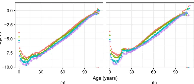
Fig. 1. Log-mortality rates for the UK for selected years for (a) males and (b) females (source: Human Mortality Database (2018)): , 1961; , 1981; , 2001; , 2013
adjusted for births, deaths and migration in the intervening period. The appropriate exposures to risk, which are needed for the calculation of mortality rates, can be estimated from these population counts. Most often, the estimated mid-year population totalsPx.t+0:5/are used to approximate exposures Rxt, directly, over the whole year under the assumption that births, deaths and migrations occur uniformly throughout the year.
The observed deaths ratesdxt=Rxt for the UK for the years 1961, 1981, 2001 and 2013 are displayed in Fig. 1, based on data taken from the human mortality database (Human Mortality Database, 2018). The human mortality database uses a more sophisticated method of approx-imating exposure to risk than that described above, accounting for the distribution of deaths within single years of age (Wilmouthet al., 2017). The mortality rates plotted can be seen to decrease with time, and consistently to increase with age beyond early adulthood, as might be expected. The empirical rates appear volatile at higher ages where there are fewer survivors and therefore less data.
The central mortality rate, which is the quantity which we wish to estimate and forecast, is defined as
mxt=E[dxt]=Rxt: .1/
This is equal to the force of mortality or hazard of deathμ.x/within the year and age group under the assumption that the force of mortality is constant over that interval. Thatcheret al. (1998) and Keyfitz and Caswell (2005) have provided more detail on the exact relationship between these quantities.
2.2. Models of mortality
A large part of the existing literature on stochastic mortality modelling has developed from the work of Lee and Carter (1992). This approach models the log-mortality rate log.mxt/by using an age-specific termαx, giving the mean mortality rate for each agex, and a bilinear termβxκt, where theκ-vector describes the overall pace of mortality decline, whereas theβ-coefficients describe how this decline varies by age, so that
This reduces the complexity of the forecasting problem, as only theκ-component varies over time. This can be modelled by using standard Box–Jenkins methods (most often a random walk with drift), which also provide for measures of forecast uncertainty.
The simplicity of the Lee–Carter model has led to a large range of other adjustments and extensions. Brouhnset al. (2002), for example, estimated the parameters through maximization of a Poisson likelihood for the observed deaths rather than working with a Gaussian likelihood on the log-rates, as in Lee and Carter (1992). Renshaw and Haberman (2003a), in contrast, included multiple bilinear age–period terms to capture a greater proportion of the total variation than is possible with a single term.
Renshaw and Haberman (2006) went further by adding a cohort term β.2/
x γt−x to allow for differences in mortality by year of birth. Models that include cohort terms are attractive as in some countries, and notably in the UK, cohort effects are prevalent in the underlying mortality data, possibly reflecting the different life experiences and lifestyle habits of those born in different periods (Willets, 2004; Cairns et al., 2009). Standard age–period–cohort (APC) models can therefore capture such characteristics of the data but, given the linear dependence in such models (in thatc=t−x, withcindexing cohort), identifying constraints are needed for fitting. APC models are widely used in the field of cancer research to make predictions of future cancer rates (e.g. Mølleret al. (2003)).
The work of Cairns and collaborators (Cairnset al., 2009; Dowdet al., 2010) describes a family of models where mortality is modelled through sums of terms of the form βxκtγt−x, where βx refers to age effects, κt to period effects andγt−x to cohort effects. Any of these elements may be constant or deterministic in particular models, and so the Lee–Carter and APC models are incorporated as special cases. The in-sample and forecasting performance of these models were assessed against a number of criteria in Cairnset al. (2009). A notable finding was the lack of robustness of many of the models that were investigated that included cohort effects; in particular, parameters in such models were found to be sensitive to the fitting period. Furthermore, Palin (2016) has identified some concerns regarding potentially spurious quadratic patterns in cohort effects in several of the models that were discussed above, caused by variation in mortality improvement rates by age being captured in the cohort effect.
Renshaw and Haberman (2003b) identified commonalities between the Lee–Carter model and their generalized linear model approach to mortality modelling focusing on mortality reduc-tion factors. Instead of modelling declines in mortality by using a bilinear termbxκt, however, Renshaw and Haberman included a termbxtthat is linear in time, simplifying the fitting process. Thebx-parameters now represent age-specific mortality improvements, where improvements are defined as differences in log-mortality. In a similar vein, and building on the cohort enhancement proposed by Renshaw and Haberman (2006), an APC model for improvements has been de-veloped by the Continuous Mortality Investigation (2016). However, this forces a deterministic convergence to user-specified long-term rates of mortality improvement rather than using time series methods for forecasting. Richardset al. (2017), however, have provided full stochastic forecasts by using the APC for improvements model by fitting time series models to the period and cohort effects, and also found that this model fits the data better in sample than either the APC or Lee–Carter models.
function coefficients that was used in theP-spline method to ensure smoothness in sample also provides for extrapolation. Although this model fits the data well, forecasts that are wholly dependent on extrapolation from splines are likely to be oversensitive to data and trends at the forecast origin.
Bayesian methods are also increasingly being employed for mortality forecasting to incor-porate prior knowledge about underlying processes, and to provide distributions of future mortality risk accounting for multiple sources of uncertainty. Girosi and King (2008) demon-strated methods for mortality forecasting within a Bayesian framework that allow for smoothing the underlying data together with borrowing strength across regions, as well as jointly forecast-ing cause-specific mortality. Wi´sniowskiet al. (2015) used the Lee–Carter method for all three components of demographic change (fertility, mortality and migration), again using Bayesian methods to obtain predictive probability distributions.
The method that is developed in this paper combines elements of many of the approaches above, including allowing for smooth functions of age and cohort, while providing stable esti-mates of mortality at extreme ages and avoiding some of the problems that are caused by lack of robustness in parameter estimation that was discussed above. The model also shares some features with the APC for improvements model of Richards et al. (2017), particularly in the structure of the main part of the model. However, there are some significant points of differ-ence; the model that is described here applies to the entire age range and adopts a Bayesian approach to account for all sources of uncertainty.
2.3. Structure
The remainder of the paper is structured as follows: Section 3 sets out the features of the model that are used in later sections. Section 4 details the data that are used and the estimation procedure. Section 5 presents the posterior distributions of the GAM components and provides predictive distributions for log-rate forecasts, and Section 6 displays posterior distributions combined over several alternative models on the basis of in-sample predictive performance, using the method of Yaoet al. (2018). Section 7 presents an alternative model where the sexes are fitted jointly, whereas Section 8 compares out-of-sample performance of the single-sex and joint models, using the years 2004–2013. Section 9 contrasts forecasts from the joint model with those made by the UK Office for National Statistics (ONS) (Office for National Statistics, 2016), and the final section offers some conclusions and directions for future work.
The programs that were used to analyse the data can be obtained from
http://wileyonlinelibrary.com/journal/rss-datasets
3. Model description
3.1. Bayesian generalized additive models
GAMs provide a flexible framework for modelling outcomes where the functional form of the response to covariates is not known with certainty but is expected to vary smoothly. The general form for such models is as follows (Wood, 2006):
g{E.yi/}=xiθ+s1.xi1/+s2.xi2/+: : : :
strictly local basis functions, with the domain of each function defined by a set of knots spread across the covariate space (Wood, 2016). Following the BayesianP-splines approach of Lang and Brezger (2004), prior distributions are used to represent a belief that adjacent P-spline covariates β will be close to one another. Multivariate normal prior distributions are used, with the covariance matrix constructed from two matrices:Aproviding a penalty on the first differences of the vector of coefficientsβ, andBpenalizing the null space ofAensuring that the resulting prior is proper (Wood, 2016):
s.x/=βTb.x/,
β∼MVN
0,
1
σ2 A
A+σ12
B B
−1
: .3/
3.2. Generalized additive models for mortality forecasting
The method of mortality forecasting that is developed in this paper fits a GAM to the majority of the age range, while applying separate parametric models to older age groups and to infants. This enables a flexible but smooth fit where the data allow and imposes some structure on the model where data are sparse, particularly at very high ages. Deathsdxtare considered to follow a negative binomial distribution parameterized in terms of the mean, which in this case is equal to the product of the relevant exposureExtand expected death ratemxt. The dispersionφcaptures additional variance relative to the Poisson distribution:
dxt∼NegBinomial.Extmxt,φ/,
p.dxt|mxt,Ext,φ/=
Γ.dxt+φ/
dxt!Γ.φ/
Extmxt
Extmxt+φ
dxt φ
Extmxt+φ
φ
:
An APC GAM for the log-mortality improvement ratios log.mxt=mx.t−1//could be expressed with P-spline-based smooth functions for age and cohort improvements, and an additional period componentκ:
log
mxt
mx.t−1/
=sβ.x/+sÅγ.t−x/+κÅt : .4/
An equivalent expression of this model can be made in terms of mortality rates rather than mortality log-improvement-ratios
log.mxt/=sα.x/+sβ.x/t+sγ.t−x/+κt, .5/ with the cohort and period terms now accumulated versions of their equivalents in equation (4). This is the model that is used in the estimation process. There are now two smooth functions of age:sα.x/, which describes the underlying shape of the log-mortality curve, andsβ.x/, which describes the pattern of (linear) mortality improvements with age. Knots are spaced at regular intervals in both the age and the cohort direction (every 4 years), with three knots placed outside the range of the data at either end of the age range, enabling a proper definition of theP-spline at the edge of the data.
T
t=1
κt=0, T t=1
tκt=0,
C
c=1
sγ.c/=0, sγ.1/=0, sγ.C/=0,
.6/
withChere indicating the most recent cohort andT the latest year. These constraints ensure that linear improvements in mortality with time are estimated as part of thesβ.x/term.
For older ages, a parametric model is adopted because of the sparsity of the data in these regions—the additional structure that is provided by specifying a parametric form guards against overfitting and instabilities in this age range:
mxt=
exp.β0old+β1oldx+β2oldt+β3oldxt/
1+exp.β0old−log.ψ/+β1oldx+β2oldt+β3oldxt/ exp{sγ.t−x/+κt} ∀x:xxold:
.7/
A logistic form is used, allowing mortality rates to tend towards a constantψas age increases, as in the model in Beard (1963). Such a pattern in mortality at the population level has some theoretical justification, as it can result when heterogeneity (‘frailty’) is applied to rates that follow a log-linear Gompertz mortality model at the individual level, and this frailty is assumed to be distributed among the population according to a gamma distribution (Vaupelet al., 1979). In the life table context, Doddet al. (2018a) found that the logistic form performed better than the log-linear equivalent when assessed by using cross-validation techniques. Linear age and time effects are included in the old age model, together with an interaction term, and the cohort and period effects are held in common with the model that is applied to younger ages and are applied multiplicatively to the logistic model.
Constraints are also applied to the parameters of the old age model to ensure that the derivative of the parametric part of the model with respect to age (ignoring the period and cohort effects) is never less than 0; this reflects our prior belief that mortality should not decrease with age after middle age. The constraints that are required are as follows, withHdescribing the most distant time for which forecasts are desired:
βold 1 >0,
βold 2 <0,
βold
3 >−β1old=H:
⎫ ⎬
⎭ .8/
Infant mortality is also excluded from the GAM, as it behaves differently from mortality at other ages. The model for infants is given a similar structure to the old age model, except that the period effectκt is excluded, as variation in infant mortality with time does not appear to follow the same pattern as it does over the rest of the age range:
log.m0t/=β10+β01t+sγ.t/: .9/
The period-specific effectsκt in equations (5) and (7) are common across ages and capture deviations from the linear trend that is described by the smooth improvementssβ. These effects are not modelled as smooth, as they may capture effects such as weather conditions or infec-tious disease outbreaks that would not be expected to vary smoothly from year to year. The innovations in these period effects are given a normal prior with varianceσκ, so that
κt=κt−1+ t,
However, these effects are constrained to identify the APC model, so we need to account for this by conditioning on the two period constraints that are given in equation (6). This is achieved by transforming the-parameters by using a matrixZ, constructed so that the final T−2 parameters remain unchanged, but the first two transformed parameters will equal 0 if the constraints on the cumulative sum of the-series hold (see the on-line appendix). The resulting vectorηhas a multivariate normal distribution
η=Z,
η∼MVN.0,ZZTσκ2/: .
11/
A distribution conditioning on the first two elements ofη, denotedη†, equalling 0 can be obtained by using standard results for the multivariate normal distribution. This conditional prior onηÅ (which contains the last T−2 elements ofη) is the distribution that is used for sampling, and the full set of values ofcan then be recovered deterministically:
η=
η† ηÅ
,
ηÅ|.η†=0/∼N.0,Σ
ÅÅ−ΣņΣ−1††Σ†Å/,
Σ=ZZTσ2, =Z−1
0 ηÅ
,
⎫ ⎪ ⎪ ⎪ ⎪ ⎪ ⎪ ⎬ ⎪ ⎪ ⎪ ⎪ ⎪ ⎪ ⎭
.12/
where subscripts on the covariance matrices indicate partitions, soΣņis the submatrix ofΣ
with rows corresponding toηÅ and columns toη†. For forecasts, innovations of the period coefficients are unconstrained and so have independent normal distributions with varianceσκ2. The same method is used to define a distribution for the innovations in the basis functions coefficients for the cohort spline, accounting for the cohort constraints in equation (6) and replacing the prior in expression (3). In contrast with the period effects, however, the trans-formation matrix that is used accounts for the fact that the constraints apply to the resulting smooth function and not the coefficient values themselves. Knots for the basis functions of the cohort smooth are evenly spaced along the range of cohorts to be estimated, so forecasts of future cohort values can be obtained by drawing new coefficient innovations from the normal distribution with mean 0 and varianceσ2γwhich replacesσA2 andσ2Bfor this effect. Full details are given in the on-line appendix.
Priors for the model hyperparameters are generally vague, although not completely uninfor-mative:
βold∼N.0, 100/,
β0∼N.0, 100/,
σA∼N+.0, 100/,
σB∼N+.0, 100/,
σκ∼N+.0, 100/,
σγ∼N+.0, 100/,
φ∼U.−∞,∞/,
ψ∼LogNormal.0, 1/:
Carlo samples, but with reasonable amounts of data should not affect the final inference to any great extent (Gelmanet al., 2014). The scale of the data and covariates is also important in determining the interpretation of these priors; the use of standardized age and time indices means that regression coefficients are unlikely to take large values. The use of the addition symbol as a subscript appended to the normal distribution,N+, indicates that only the positive part of the normal distribution is used and therefore refers to a half-normal distribution.
4. Estimation
Samples from the posterior distributions of the parameters and rates were drawn by using Hamil-tonian Monte Carlo sampling and specifically using thestansoftware package (Stan Develop-ment Team, 2015).stanand its interface in the R programming language (R Core Team, 2017) allows the construction of a Hamiltonian Monte Carlo sampling ‘no U-turns sampler’ (Hoff-man and Gel(Hoff-man, 2014) from a simple user specification of the Bayesian model to be estimated. The code that is required to fit the model is also available from https://github.com/
jasonhilton/mortality-bgam.Hamiltonian Monte Carlo sampling is a special case of
the more general Metropolis–Hastings algorithm for Markov chain Monte Carlo sampling and uses the derivatives of the log-posterior with respect to the parameters of interest in the sampling process, often enabling the posterior to be traversed much more quickly than under standard methods (Neal, 2010). The model was fitted using human mortality database data for the UK from 1961 to 2013 (Human Mortality Database, 2018). The first five cohorts (those born be-fore 1856) were excluded, as exposures are very low for these groups. Four parallel chains were constructed, each with 8000 samples, and the first half of each chain was used as a warm-up period (during whichstantunes the algorithm to reflect the characteristics of the posterior best) and discarded. Parallel chains were used to assess convergence to the posterior distribution better; the diagnostic measure that was advocated by Gelman and Rubin (1992) indicates that all parameters have converged to an acceptable degree. The 16000 post-warm-up samples were ‘thinned’ by a factor of 4 by discarding three values in four to avoid excessive memory usage, leaving 4000 posterior samples for inference for each model.
5. Initial results
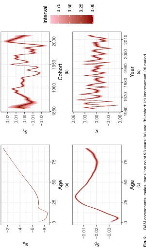
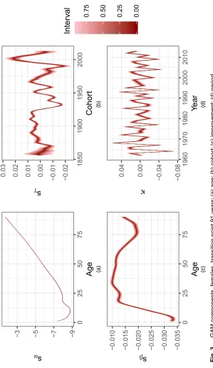
Some preliminary results are displayed in this section, conditionally on a particular choice for the point of transition between the GAM to the parametric old age model. Fitting a similar model to ONS data for England and Wales for 2010–2012, Doddet al. (2018a) found by using cross-validation methods that the most probable points of transition were age 91 for females and 93 years for males. Samples were obtained for models using these transition points, and the posterior distributions of the parameters of the GAM model are given in Figs 2 and 3 for males and females respectively. The colour scheme in these plots identifies intervals containing vari-ous proportions of the posterior density, so that the darkest represents the central 2% interval, whereas 90% of the posterior density is contained between the lightest bands. The distribu-tions of mortality improvement rates for both males and females display greater uncertainty at younger ages where there are fewer deaths. As might be expected, uncertainty for cohort effects increases for the oldest and most recent cohorts, as these have the fewest data points. Note that it is the differenced cohort and period effects (sÅγ.t−x/andκÅt from equation (4)) that are plotted rather than their summed equivalents.
−8 −6 −4 −2 02 5 5 0 7 5
Age
(a [image:9.485.87.388.82.593.2]0 40 80
(a) (b)
120 0 40 80 120
−12 −9 −6 −3 0
Age (years)
Log-rate
[image:11.485.49.443.55.282.2]0.00 0.25 0.50 0.75 Interval
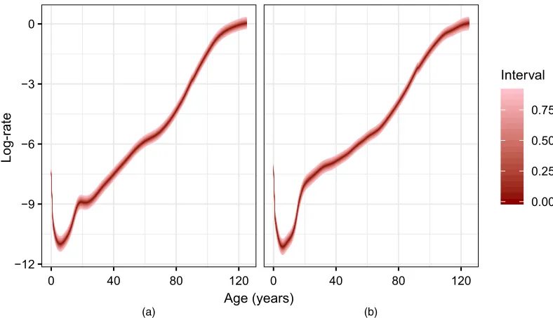
Fig. 4. Predictive distribution of log-rates with single points of transition, 2063: (a) females; (b) males
show lower rates of improvement than females in their late 20s. Cohort and period contributions to mortality decline show similar but not identical patterns for each sex.
Posterior distributions for log-rates generated from this model fit the data relatively closely. However, Fig. 4 displays forecasts of log-rates at 50 years into the future, which, although appearing reasonable, contain small discontinuities at the point of transition between the GAM and the parametric model. The discontinuity is particularly evident in the forecast for males. This suggests that some sort of averaging over or combination of models using different transition points might be advisable.
6. Transition points and model stacking
The choice that is made regarding the age at which the model transitions from the GAM (which is used over the majority of the age range) to the parametric model for old ages is essentially arbitrary; we do not believe that there is a switch between data-generating processes at some pointxold, but rather that the task of predicting mortality is better served by two models. There
is thus no ‘true’ value for the point of transition, and decisions regarding transition should be governed by model performance. The methodology that was used in the latestEnglish Life Tables (Doddet al., 2018a) used cross-validation to obtain posterior weights over a set of modelsM defined byKdifferent points of transition, based on mortality data from 2010 to 2012. In that analysis, age 91 for females and 93 years for males are the most probable points of transition, and the final predictive distribution was obtained by averaging over models using the calculated weights. However, the model that is described here differs from that used in Doddet al. (2018a) in that it varies in time and applies to a period spanning many years, so the question of the distribution of the transition between the parametric model and the GAM must be revisited.
58890 58920 58950 58980 59010
80 85 90 95
Transition Point
(a) (b)
LOOIC
60175 60200 60225 60250
80 85 90 95
Transition Point
[image:12.485.44.439.52.246.2]LOOIC
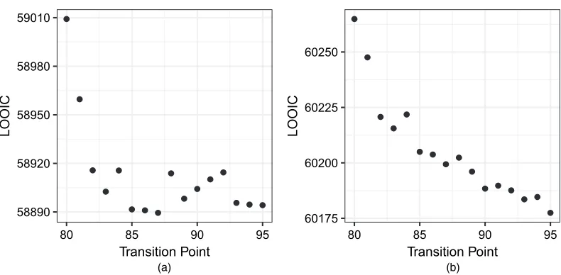
Fig. 5. LOOIC values for models by using different transition points: (a) females; (b) males
developed by Vehtariet al. (2016). The LOOIC is a measure of how well we might expect a model to perform in predicting a data point without including it in the data that are used to fit the model. It is based on an approximation of the leave-one-out log-pointwise predictive density Σn
i=1log{p.yi|y−i/}, where they−isubscript indicates a data set excluding theith observation,
θis a vector of parameters and
p.yi|y−i/=
p.yi|θ/p.θ|y−i/dθ:
Rather than fitting the modelntimes (once for every data point), Vehtariet al. (2016) provided a method for approximating the LOOIC from just one set of posterior samples of the predictive density computed from the full data set, implemented within the looR package. This uses importance sampling to approximate the leave-one-out log-predictive-density, correcting for instabilities caused by the potentially high or infinite variance of some importance weights by fitting a Pareto distribution to the upper tail of the raw weights.
The LOOIC scores for males and females for the models with transition points k=[80,
81,: : :, 95] years are given in Fig. 5. Later cut points tend to be preferred because the greater
flexibility of the GAM model gives lower LOOIC values even at relatively high ages, although the absolute differences between the models are small. Models with points of transition above age 95 years are not considered, as this would leave too few data points with which to estimate the old age model effectively.
Although the LOOIC is not a measure offorecastperformance as such, as it is focused on how the model would perform at predicting data points that are contained within the original data set and does not consider the times at which data points become available, it does provide an indication of how well the models specified reflect the structure of the data.
Following the work by Yaoet al. (2018), these LOOIC values can be used as the basis for ‘stacking’ the predictive distributions of each model to obtain a distribution which combines models in a principled way, with weights determined by approximate cross-validation perfor-mance. Stacking is often used for averaging over point estimates in ensemble models, but Yao
0.00 0.05 0.10 0.15 0.20
80 85 90 95
Point of Transition
Model W
eight
0.0 0.2 0.4
80 85 90 95
Point of Transition
Model W
eight
[image:13.485.48.446.52.248.2](a) (b)
Fig. 6. LOOIC values for models by using different points of transition: (a) females; (b) males
0 40 80
(a) (b)
120 0 40 80 120
−12 −8 −4 0
Age
Log-r
ate
[image:13.485.50.444.243.486.2]0.00 0.25 0.50 0.75 Interval
Fig. 7. Stacked forecasts for 2063, single-sex models: (a) females; (b) males
weightsw, elements of which correspond to one ofKpossible modelsMk, are estimated through the solution of the optimization problem
arg max
w n
i=1 log
K
k=1
wkp.yi|y−i,Mk/
subject towk>0, K k=1
wk=1, .13/
(Yaoet al. (2018), page 7), wherep.yi|y−i,Mk/is approximated by using the LOOIC measure
described above. The form of the combined predictive distribution is then
ˆ
p.y˜|y/=K
k=1
The estimated model weights are shown in Fig. 6; the greatest individual weight is given to models with the latest points of transitions, reflecting the pattern in the LOOIC measure. Other models with earlier transition points are also given weight, however, reflecting that they perform well at predicting some data points which are not so well estimated by the late transition model. Samples from the combined posterior predictive distribution were obtained by using the estimated weights by sampling from the posterior distribution that is associated with each model in proportion to its weight. The resulting stacked forecasts are given in Fig. 7; the discontinuities that were seen previously are now smoothed out through the process of taking the weighted combination of distributions.
7. Jointly modelling male and female mortality
In the work that was described above, models for males and females were estimated separately. However, much of what drives the underlying processes of mortality and how it changes over time is likely to be common between sexes. Thus, we may gain from borrowing strength across models and also from explicitly representing covariances between parameters for each sex, as in Wi´sniowskiet al. (2015). Because males tend to die sooner than females, there are fewer data points (i.e. lower total exposure) with which to estimate parameters in the old age model. For this reason, the parameterψ, representing the asymptote of the logistic function in the old age model, is now shared between sexes.
We also allow the innovations in the period effectsκtto be correlated, so that joint forecasts can be generated accounting for the fact that, in potential futures where mortality for females is high, it will tend to be high for males as well. The joint distribution for the period innovations for both sexes, conditionally on the constraints, is obtained in a similar way to that for the single-sex models, described in Section 3. Full details are given in the on-line appendix.
As before, LOOIC scores and model weights were obtained for the joint model (Fig. 8). The pattern of LOOIC scores and weights are similar to those for the separate models, with the highest transition point obtaining most weight, but considerable weight also attached to earlier transitions.
119100 119150 119200 119250
80 85 90 95
Point of Transition
(a) (b)
LOOIC
0.0 0.1 0.2 0.3
80 85 90 95
Point of Transition
[image:14.485.48.442.421.614.2]Model weight
0 40 80
(a) (b)
120 0 40 80 120
−9 −6 −3 0
Age
Log-r
ate
[image:15.485.45.448.54.260.2]0.25 0.50 0.75 Interval
Fig. 9. Stacked forecasts from the joint-sex model, 2038: (a) females; (b) males
Joint forecasts of log-mortality are displayed in Fig. 9. The estimated correlation in the inno-vations of the period effects (the off-diagonal elements ofP) is high—generally above 95%.
8. Model assessment
To assess the robustness and forecasting accuracy of the models that were described above, fitting was conducted on a truncated data set, excluding the years 2004–2013. Robustness was then assessed by comparing posterior means of the main smooth functions estimated on this reduced data set against the same quantities estimated on all the data. Fig. 10 displays such a comparison for males, plotting posterior means for each point of transition and fitting period. Estimates of period and cohort effects are relatively stable, particularly in the interior of the data. Although some differences are evident in the pattern of improvements, the general shape of the curve is notably similar, and the downward shift appears to reflect real increases in the rate of mortality decline after 2003, particularly for younger adults. The shape of the age effect is again very similar, and the differing location of the smooth curve is accounted for by a change in the location of the intercept of the time index in equation (5) for different data periods.
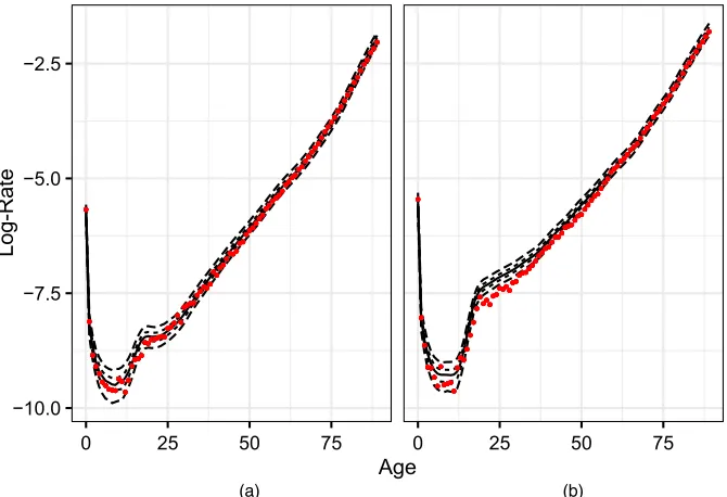
Both the single- and the joint-sex models that were presented above appear to give reasonable forecasts for future mortality. Figs 11 and 12 display predictive distributions and empirical rates for younger and older ages respectively. Comparing the predictive posterior distributions against the observed outcomes, it is evident that, for most of the age range, empirical rates fall within the 90% predictive interval. The exception is young adult males, between the ages of about 15 and 40 years, for whom recent drops in mortality far outpace those seen in the observed data 1961–2003. More formal assessments of forecast performance are difficult, as we observe only one correlated set of outcomes (i.e. male and female log-rates 2004–2013).
−8 −6 −4 −2
0 25 50 75
Age
sα
−0.02 −0.01 0.00 0.01 0.02
1850 1900 1950 2000
Cohort
sγ
−0.03 −0.02 −0.01 0.00
0 25 50 75
Age
sβ
−0.050 −0.025 0.000 0.025 0.050
1960 1970 1980 1990 2000 2010
Age
κ
(a) (b)
[image:16.485.45.438.50.302.2](c) (d)
Fig. 10. Comparison of posterior means of GAM components for various fitting periods ( , 1961–2003; , 1961–2013) and transition points, males: (a) age; (b) cohort; (c) improvement; (d) period
0 25 50
(a) (b)
75 0 25 50 75
−10.0 −7.5 −5.0 −2.5
Age
Log-Rate
[image:16.485.75.410.376.605.2]80 90 100 110 80 90 100 110 −3
−2 −1 0 1
−3 −2 −1 0 1
Age
Log-Rate
(a) (b)
[image:17.485.81.417.55.311.2](c) (d)
Fig. 12. Comparison of posterior predictive distributions for old-age log-rates against empirical observa-tions, (a), (b) 2008 and (c), (d) 2013, single- ( ) and joint-sex ( ) models ( , median; , 0.5 percentile; , 0.9 percentile): (a), (c) females; (b), (d) males
similar properties. Other considerations may be taken into account when deciding between the two models; the joint model is more parsimonious in that fewer parameters are required to fit it, and it allows for correlations in the paths of mortality by sex to be taken into account. In contrast, the single-sex model is less computationally demanding, particularly with respect to memory, as each sex is fitted and processed separately.
9. Comparison with offical projections and variants
The final stacked forecasts from the joint model in the previous section are now compared with forecasts that are produced by the UK ONS in the 2014-based national population projections (NPPs) (Office for National Statistics, 2016). These work with the predicted probabilities of deathsqxrather than the central mortality ratesmx; the former represents the probability of dying by agex+1 given that an individual attains agex. Posterior predictive samples ofqxtwere acquired by using the approximation
qxt≈1−exp.−mxt/: .14/
As well as the principal ONS projection from the 2014-based NPP, the variant projections involving high and low mortality scenarios have been included, allowing some understanding of how the existing indications of uncertainty resulting from different projection assumptions compare with the fully Bayesian probability distributions.
-0 40 80
(a) (b)
120 0 40 80 120
−10.0 −7.5 −5.0 −2.5 0.0
Age
Log q(x)
0.00 0.25 0.50 0.75
[image:18.485.43.438.47.258.2]Interval
Fig. 13. Forecast log-probabilities of death for 2038 ( , ONS variant high; , ONS variant low; , principal ONS variant): (a) females; (b) males
2000 2025
(a) (b)
2050 2000 2025 2050
70 75 80 85 90 95
Year
e0
0.00 0.25 0.50 0.75
Interval
Fig. 14. Forecast life expectancy at birth, ONS NPP and GAM-based forecast ( , ONS variant high; , ONS variant low; , principal ONS variant): (a) females; (b) males
[image:18.485.44.440.300.532.2]greater weight that is given by the ONS methodology to more recent high improvement rates at these ages (see Office for National Statistics (2016) for more details regarding the ONS methodology).
9.1. Life expectancy
Period life expectancy at birth is a useful summary measure of the mortality conditions in a given year. It captures the expected number of years lived of a hypothetical individual who ex-periences a given period’s schedule of mortality rates over the course of their whole life. Fig. 14 compares the posterior distribution of life expectancy at birth,e0, from the jointly fitted
GAM-based model with the equivalent quantity from the NPP. The GAM-GAM-based forecasts appear more optimistic than the ONS equivalent, with median life expectancy higher than the prin-cipal ONS projection because of the lower predictions of mortality at ages 70–95 years un-der the GAM-based model. Fig. 14 also reveals that uncertainty ine0 initially grows more
quickly in the Bayesian approach that was developed above, in that the gap between the high and low variants is much narrower than the fan intervals for at least the first decade of the forecast. After 30 years, however, the range that is spanned by the ONS variants becomes wider than the 90% probabilistic interval from the GAM-based model. The uncertainty in the probabilistic forecast reflects past variability in the observed data and, from the comparison with hold-back data given in Figs 11 and 12, the calibration of this uncertainty appears rea-sonable. As a result, we believe that the probabilistic intervals provide a better indication of the uncertainty around future life expectancy than the scenario-based equivalents, at least in the short term, particularly as they have a readily understandable interpretation in terms of probability.
10. Discussion and conclusion
This paper details methodology for the fully probabilistic forecasting of mortality rates, ac-counting for uncertainty in parameter estimates as well as in forecasting. The approach uses a GAM to produce smooth rate estimates at younger ages and combines this with a parametric model at higher ages where the data are more sparse, allowing rate estimates to be obtained for extreme old ages. The use of Hamiltonian Monte Carlo sampling and thestansoftware package allowed posterior sampling to be conducted with reasonable efficiency.
Stacking predictive distributions following the approach of Yaoet al. (2018) provides a prin-cipled approach to avoiding a single choice of transition point between these two submodels governing younger and older age ranges. These weights are based on approximate leave-one-out cross-validation performance and thus weight models on the basis of their ability to predict data that are contained in the original fitting period. An alternative approach may be to fit models on a subset of data, and to produce weights based on model performance in forecasting data at the end of the time period. However, this would involve additional model refitting, and it may also be that such assessments are overly sensitive to characteristics of the held-out data. Further-more, log-scores based on a single set of observed outcomes are likely to be highly correlated, and thus rollingn-step-ahead forecasts may be required to assess forecast performance robustly, which would necessitate repeated model fitting with even greater computational expense.
Future work could investigate the inclusion of expert opinion in probabilistic mortality fore-casting models like that presented in this paper. The NPP uses experts to provide target rates of mortality improvement over longer time horizons (25 years) (Office for National Statistics, 2016), reflecting the fact that extrapolative methods may prove inferior to expertise at this dis-tance into the future. A similar approach within a Bayesian framework would have to consider that using expert opinion about future rates is different from the standard approach of eliciting information about model parameters directly. Work in Doddet al. (2018b) describes one way in which this could be achieved. Beyond this, there are also opportunities to investigate the possi-bility of extending similar methods to other demographic components, particularly fertility.
Acknowledgements
This work was supported by the Economic and Social Research Council Centre for Population Change—phase II (grant ES/K007394/1) and a research contract to review the methodology for projecting mortality between the ONS and the University of Southampton. The use of the IRIDIS High Performance Computing Facility, and associated support services at the Univer-sity of Southampton, in the completion of this work is also acknowledged. Earlier work on this model was presented at a joint Eurostat–United Nations Economic Commission for Europe work session on demographic projections (Forsteret al., 2016). All the views presented in this paper are those of the authors only.
References
Beard, R. (1963) A theory of mortality based on actuarial, biological, and medical considerations. InProc. Int. Population Conf., pp. 611–625. New York: International Union for the Scientific Study of Population. Brouhns, N., Denuit, M. and Vermunt, J. K. (2002) A Poisson log-bilinear regression approach to the construction
of projected lifetables.Insur. Math. Econ.,31, 373–393.
Cairns, A. J. G., Blake, D., Dowd, K., Coughlan, D., Epstein, D. and Ong, A. (2009) A quantitative comparison of stochastic mortality models using data from England and Wales and the United States.Nth Am. Act. J.,13, 1–35.
Continuous Mortality Investigation (2016) CMI mortality projections model consultation. Working Paper 90. Institute and Faculty of Actuaries, London. (Available from https://www:actuaries.org.uk/ documents/cmi-working-paper-90-cmi-mortality-projections-model-consultation.) Currie, I. D., Durban, M. and Eilers, P. H. C. (2004) Smoothing and forecasting mortality rates.Statist. Modllng,
4, 279–298.
Dodd, E., Forster, J. J., Bijak, J. and Smith, P. W. F. (2018a) Smoothing mortality data: theEnglish Life Tables, 2010–2012.J. R. Statist. Soc.A,181, 717–735.
Dodd, E., Forster, J. J., Bijak, J. and Smith, P. W. F. (2018b) Stochastic modelling and projection of mortality improvements using a hybrid parametric/semiparametric age-period-cohort model. University of Southampton, Southampton. (Available fromhttps://eprints.soton.ac.uk/42219/.)
Dowd, K., Cairns, A. J. G., Blake, D., Coughlan, G. D., Epstein, D. and Khalaf-Allah, M. (2010) Evaluating the goodness of fit of stochastic mortality models.Insur. Math. Econ.,47, 255–265.
Forster, J. J., Dodd, E., Bijak, J. and Smith, P. W. F. (2016) A comprehensive framework for mortality fore-casting.Jt Eurostat–United Nations Economic Commission for Europe Work Session Demographic Projections, Geneva.
Gelman, A., Carlin, J. B., Stern, H. S., Dunson, D. B., Vehtari, A. and Rubin, D. B. (2014)Bayesian Data Analysis, 3rd edn. Abingdon: CRC Press.
Gelman, A. and Rubin, D. B. (1992) Inference from iterative simulation using multiple sequences.Statist. Sci.,7, 457–472.
Girosi, F. and King, G. (2008)Demographic Forecasting. Princeton: Princeton University Press.
Hoffman, M. D. and Gelman, A. (2014) The no-U-turn sampler: adaptively setting path lengths in Hamiltonian Monte Carlo.J. Mach. Learn. Res.,15, 1–31.
Human Mortality Database (2018) Human mortality database. Max Planck Institute for Demographic Research, Rostock. (Available fromhttp://www.mortality.org.)
Keyfitz, N. and Caswell, H. (2005)Applied Mathematical Demography, 3rd edn. New York: Springer. Lang, S. and Brezger, A. (2004) Bayesian P-splines.J. Computnl Graph. Statist.,13, 183–212.
Lee, R. D. and Carter, L. R. (1992) Modeling and forecasting U.S. mortality.J. Am. Statist. Ass.,87, 659– 671.
Møller, B., Fekjær, H., Hakulinen, T., Sigvaldason, H., Storm, H. H., Talb¨ack, M. and Haldorsen, T. (2003) Prediction of cancer incidence in the Nordic countries: empirical comparison of different approaches.Statist. Med.,22, 2751–2766.
Neal, R. (2010) MCMC using Hamiltonian Dynamics. InHandbook of Markov Chain Monte Carlo(eds S. Brooks, A. Gelman, G. Jones and X.-L. Meng). Boca Raton: Chapman and Hall–CRC.
Office for National Statistics (2016) National population projections: 2014-based reference volume, series PP2.
Technical Report. Office for National Statistics, Newport. (Available fromhttps://www.ons.gov.uk/ peoplepopulationandcommunity/populationandmigration/populationprojections/com pendium/nationalpopulationprojections/2014basedreferencevolumeseriespp2.) Palin, J. (2016) When is a cohort not a cohort?: Spurious parameters in stochastic longevity models. InProc. Int.
Mortality and Longevity Symp.London: Institute and Faculty of Actuaries.
R Core Team (2017)R: a Language and Environment for Statistical Computing. Vienna: R Foundation for Statistical Computing.
Renshaw, A. and Haberman, S. (2003a) Lee–Carter mortality forecasting with age-specific enhancement.Insur. Math. Econ.,33, 255–272.
Renshaw, A. and Haberman, S. (2003b) Lee–Carter mortality forecasting: a parallel generalized linear modelling approach for England and Wales mortality projections.Appl. Statist.,52, 119–137.
Renshaw, A. and Haberman, S. (2006) A cohort-based extension to the Lee-Carter model for mortality reduction factors.Insur. Math. Econ.,38, 556–570.
Richards, S. J., Currie, I. D., Kleinow, T. and Ritchie, G. P. (2017) A stochastic implementation of the APCI model for mortality projections.Sessional Research Paper. Actuarial Research Centre, Institute and Faculty of Actuaries, London. (Available from https://www.actuaries.org.uk/documents/ stochastic-implementation-apci-model.)
Stan Development Team (2015)Stan Modeling Language Users Guide and Reference Manual.
Thatcher, A. F., Kannisto, V. and Vaupel, J. W. (1998)The Force of Mortality at Ages 80-120. Odense: Odense University Press.
Vaupel, J. W., Manton, K. G. and Stallard, E. (1979) The impact of heterogeneity in individual frailty on the dynamics of mortality.Demography,16, 439–454.
Vehtari, A., Gelman, A. and Gabry, J. (2016) Practical Bayesian model evaluation using leave-one-out cross-validation and WAIC.Statist. Comput.,27, 1–20.
Willets, R. C. (2004) The cohort effect: insights and explanations.Br. Act. J.,10, 833–877.
Wilmouth, J. R., Andreev, K., Jdanov, D., Glei, D. A. and Riffe, T. (2017) Methods protocol for the human mor-tality database.Technical Report. Human Mortality Database. (Available fromhttp://www.mortality. org/Public/Docs/MethodsProtocol.pdf.)
Wi´sniowski, A., Smith, P. W. F., Bijak, J., Raymer, J. and Forster, J. J. (2015) Bayesian population forecasting: extending the Lee-Carter method.Demography,52, 1035–1059.
Wood, S. N. (2006)Generalised Additive Models: an Introduction with R. Boca Raton: Chapman and Hall–CRC. Wood, S. N. (2016) Just another Gibbs additive modeller: interfacing JAGS and mgcv.arXiv Preprint. University
of Bath, Bath. (Available fromhttp://arxiv.org/abs/1602.02539.)
Yao, Y., Vehtari, A., Simpson, D. and Gelman, A. (2018) Using stacking to average Bayesian predictive distributions.Baysn Anal., to be published.
Supporting information