warwick.ac.uk/lib-publications
Original citation:
Sanchez Silva, Victor and Hernandez-Cabronero, Miguel (2018) Graph-based rate control in
pathology imaging with lossless region of interest coding. IEEE Transactions on Medical
Imaging . p. 1. doi:10.1109/TMI.2018.2824819
Permanent WRAP URL:
http://wrap.warwick.ac.uk/101996
Copyright and reuse:
The Warwick Research Archive Portal (WRAP) makes this work by researchers of the
University of Warwick available open access under the following conditions. Copyright ©
and all moral rights to the version of the paper presented here belong to the individual
author(s) and/or other copyright owners. To the extent reasonable and practicable the
material made available in WRAP has been checked for eligibility before being made
available.
Copies of full items can be used for personal research or study, educational, or not-for-profit
purposes without prior permission or charge. Provided that the authors, title and full
bibliographic details are credited, a hyperlink and/or URL is given for the original metadata
page and the content is not changed in any way.
Publisher’s statement:
“© 2018 IEEE. Personal use of this material is permitted. Permission from IEEE must be
obtained for all other uses, in any current or future media, including reprinting /republishing
this material for advertising or promotional purposes, creating new collective works, for
resale or redistribution to servers or lists, or reuse of any copyrighted component of this
work in other works.”
A note on versions:
The version presented here may differ from the published version or, version of record, if
you wish to cite this item you are advised to consult the publisher’s version. Please see the
‘permanent WRAP URL’ above for details on accessing the published version and note that
access may require a subscription.
Graph-based Rate Control in Pathology Imaging
with Lossless Region of Interest Coding
Victor Sanchez,
Member, IEEE,
and Miguel Hern´andez-Cabronero
Abstract—The increasing availability of digital pathology im-ages has motivated the design of tools to foster multidisciplinary collaboration among researchers, pathologists, and computer scientists. Telepathology plays an important role in the develop-ment of collaborative tools, as it facilities the transmission and access of pathology images by multiple users. However, the huge ?le size associated with pathology images usually prevents full exploitation of the collaborative telepathology system potential. Within this context, rate control (RC) is an important tool that allows meeting storage and bandwidth requirements by controlling the bit rate of the coded image. In this paper, we propose a novel graph-based RC algorithm with lossless region of interest (RoI) coding for pathology images. The algorithm, which is designed for block-based predictive transform coding methods, compresses the non-RoI in a lossy manner according to a target bit rate and the RoI in a lossless manner. It employs a graph where each node represents a constituent block of the image to be coded. By incorporating information about the coding cost similarities of blocks into the graph, a graph kernel is used to distribute a target bit budget among the non-RoI blocks. In order to increase RC accuracy, the algorithm uses a rate-lambda (R-λ) model to approximate the slope of the rate-distortion curve of the non-RoI, and a graph-based approach to guarantee that the target bit rate is accurately attained. The algorithm is implemented in the HEVC standard and tested over a wide range of pathology images with multiple RoIs. Evaluation results show that it outperforms other state-of-the-art methods designed for single images by very accurately attaining the target bit rate of the non-RoI.
Index Terms—rate-control, HEVC, pathology images, graph-based signal processing, region of interest coding.
I. INTRODUCTION
T
HE introduction of high-throughput slide scanners hasmade possible the digitization of microscope specimens to produce multi-giga pixel color images, which are usually
calledwhole-slide images(WSIs). This has fuelled the
emerg-ing area of digital pathology imagemerg-ing [1], [2].
An important aspect of digital pathology imaging is the development of efficient tools to foster multidisciplinary col-laboration among researchers, pathologists (e.g., for inter-observer concordance studies), and computer scientists (e.g., for development and validation of computer-aided diagnosis (CAD) systems). Telepathology plays an important role in the development of collaborative tools, as it facilities the transmission and access of pathology images by multiple
This work has been funded by the EU Marie Curie CIG Programme under Grant PIMCO, and the Engineering and Physical Sciences Research Council (EPSRC), UK.
V. Sanchez is with the Department of Computer Science, University of Warwick, Coventry, UK, e-mail: [email protected].
M. Hern´andez-Cabronero is with the Department of Electrical and Com-puter Engineering, University of Arizona, Tucson, Arizona 85721.
users. Specifically, through the use of telepathology, pathol-ogists can access and annotate pathology images stored in a central database, consult with distant experts, and compare annotations made by other pathologists. Similarly, computer scientists can access the ground truth provided by pathologists to design and refine their CAD systems. Such collaborative telepathology systems have been actively developed in various pathology laboratories and clinics in Europe, North America and Australia [3], [4], [5].
A key challenge that prevents fully exploiting the potential of collaborative telepathology systems is the huge file size associated with pathology images, which poses heavy demands on transmission resources. To this end, such systems initially transmit the pathology images at a low resolution to account for low bandwidth connections. The users can then select the regions of interest (RoIs), e.g., a cell, groups of cells or multi-ple tissue subregions, on which they would like to concentrate [6]. The system then transmits the RoIs at full resolution, i.e., at a higher bit rate, so the users can 1) add annotations to them, or 2) access any existing annotations. An important concern here is providing a fast and reliable transmission of the RoIs especially in low bandwidth environments. It is also important to guarantee that the RoIs are transmitted in a lossless manner, so that their clinical usage is not affected. Lossy compression in conjunction with lossless RoI coding provide an attractive solution for such cases. For instance, users with low bandwidth connections may access the RoIs at full resolution in a lossless manner while obtaining a view of the remaining regions (i.e., the non-RoI) in a lossy manner [7], [8], [9]. In this context, transmitting the necessary data at the bit rate imposed by the connection is of high importance. In other words, it is important to achieve lossless RoI coding while reducing the quality of the non-RoI according to a target bit rate. To this end, rate control (RC) is an important tool that allows meeting any bandwidth requirements. Specifically, RC allows controlling the bit rate of the non-RoI while minimizing its overall distortion. An accurate RC mechanism helps to improve the fidelity of the non-RoI, because spending too few bytes is trivially not optimal, while spending too many bytes forces truncation of the transmitted non-RoI, which may yield suboptimal fidelity.
recent ones, the work of Chen et al. in [13] proposes a two-layer system in the High-Efficiency Video Coding (HEVC) standard [11], where the enhancement layer is combined with a base layer to losslessly decode the RoI, while the base layer is used to decode the non-RoI at a lossy quality. In [15], we propose an RC algorithm in HEVC for pathology images with lossless RoI coding. This particular algorithm encodes the non-RoI by using RC and a model that approximates the corresponding rate-distortion (R-D) characteristics.
In the more general context of natural imaging data, im-portant block-based PTC methods that combine RC and RoI coding may be found in the literature [16]-[17]. The work in [16] presents a scalable RoI coding method for H.264/SVC that employs a control mechanism that adjusts the quality of the RoI and non-RoI enhancement layers. In [18], Chen et al. exploit the properties of the Human Visual System to design a foveated just-noticeable-distortion model that helps adjusting the quantization levels of RoI blocks in H.264/AVC. The work in [19] proposes a framework for RoI coding that uses a pre-processing step to replace non-RoI areas by known pixels, thus relying on the R-D optimization process to optimally encode the data. The work in [20] presents a region-based RC method aimed at improving the objective quality of high-dynamic range sequences. A similar idea is presented in [21] for intra-predicted frames. In [22], the authors present an RoI coding approach for videoconferencing that uses RC to assign more bits to blocks depicting facial features. The work in [23] proposes an RC scheme for RoI coding of screen-content videos in H.264/AVC by employing several R-D models. In [17], Meddeb et al. propose an RC algorithm for RoI coding in HEVC aimed at videoconferencing. Their algorithm assigns more bits to faces by employing two distinct R-D models.
Within the context of block-based PTC methods, the con-stituent blocks of a pathology image are usually correlated. It is then highly advisable to exploit this correlation during RC to determine the bit budget allocation that results in the set of QPs that most accurately attains a target bit rate at the highest reconstruction quality possible. The constituent blocks are then highly amenable to be represented as graphs, whose structure can be exploited during RC. Specifically, blocks can be represented as the nodes of an undirected graph and their similarities, in terms of their coding costs and region they depict, i.e., RoI vs. non-RoI, can be represented as the weight of edges that connect adjacent nodes. Based on such graph structure, we propose a graph-based RC algorithm with lossless RoI coding capabilities within the context of block-based PTC of pathology images. Our algorithm losslessly encodes RoI blocks and allocates a target bit budget among non-RoI blocks by using a graph kernel, which allows for the distribution of this bit budget according to the weights assigned to the graph edges. Based on the bit budget allocation, the QP for each non-RoI block is then computed using a model that approximates the R-D characteristics of the non-RoI. Our proposed algorithm also employs the graph structure to guarantee that the target bit budget is respected as non-RoI blocks are sequentially encoded.
Our proposed graph-based RC algorithm updates the R-D model’s parameters after encoding each non-RoI block [15],
and includes two important novel contributions:
1) Our algorithm distributes a target bit budget across the non-RoI blocks using a diffusion process on the graph representing the blocks. The advantage of this graph-based approach is that the bit budget is allocated more precisely according to the coding costs of blocks. This results in increasing the bit budget of difficult-to-code regions, while reducing the bit budget of easy-to-code regions.
2) Our algorithm also uses a graph-based approach for bit budget re-allocation; i.e., to compensate for any inaccuracies in attaining the target bit budget of each block. This is particularly useful for very large images comprising several blocks, such as pathology images, since these inaccuracies tend to amount to a large value after encoding several blocks.
It is important to mention that important methods have been recently proposed for bit budget allocation [24], [25] and re-allocation [26] in RC. Although many of these meth-ods perform very well, they are based on R-D models and optimization schemes designed for video sequences, and not single images. To the best of our knowledge, our algorithm is the first one to employ graph-based approaches in RC for bit budget allocation and to guarantee that an overall target bit budget is respected even when the target bit rate of each block is not accurately attained.
Our graph-based RC algorithm is implemented in HEVC for the coding of several pathology images using intra-prediction [27]. Results show that it outperforms other state-of-the-art approaches for single images by very accurately attaining the target bit rate of the non-RoI, while reducing blocky artifacts. The rest of the paper is organized as follows. Section II briefly reviews the R-D model used to determine the QP of each block within the context of block-based PTC. Section III details our proposed graph-based RC algorithm. Section IV presents the results on several pathology images coded at a wide range of bit rates. Section V concludes this paper.
II. RATE-DISTORTION MODEL FORRC
Most modern video and image codecs employ R-D models to approximate the distortion incurred in the reconstructed signal when coded in a lossy manner at a particular bit rate. Based on this approximation, the appropriate QP is then determined for the transform coefficients representing the signal [24], [25], [28], [15], [29], [30], [31].
In this work, we employ an R-λ model to determine
the QPs of the constituent blocks of the image within the context of block-based PTC. This particular model, which is also employed in HEVC [31], has been shown to provide a good performance with low computational complexity. It
approximates the slope of the R-D curve,λ, of a block:
λ=−∂D
∂R =αR
β, (1)
where R and D are the rate and distortion, respectively; ∂
denotes a partial derivative; andαandβare parameters related
RoI mask
Lossless compression of RoI blocks Lossless mode
Model’s parameters Graph-based bit budget allocation
Computation of QPvalues
Parameter update Lossy mode
Lossy compression of non-RoI blocks
Graph-based bit budget re-allocation Input image
[image:4.612.50.303.55.169.2]Compressed bit stream
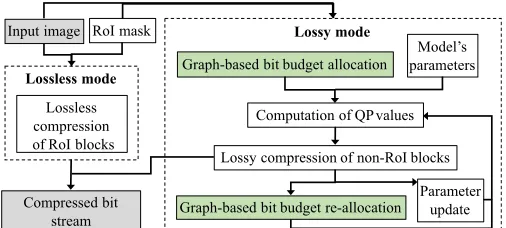
Fig. 1:Pipeline of the proposed graph-based RC algorithm.
model’s parameters [31]. The values of these parameters are usually computed from training data.
Onceλis computed for a block, the corresponding QP can
be determined using a linear relationship [32]:
QP =alogλ+b, (2)
whereaandbare also parameters whose values are computed
from training data.
It is important to note that if the approximation in Eq. 1 is accurate, the target bit rate is accurately attained for each block and thus for the whole image. However, if this approximation is inaccurate, the overall bit budget may be overspent or underspent. To improve the accuracy in attaining the target
bit rate, RC methods based on an R-λmodel usually employ
a mechanism to fine tune the model’s parameters as blocks are sequentially encoded. Specifically, the model’s parameters
are updated using the actual bit rate, Ract, and the actual λ
value, λact =αRβact, of each encoded block. After encoding
of each block, α and β are updated as a weighted average
of the model’s parameters used in previously encoded blocks [28]:
αupdated =α+δα(lnλ−lnλact)α, (3)
βupdated=β+δβ(lnλ−lnλact)β, (4)
whereδα= 0.1 andδβ = 0.05are constants that control the
updating process [28].
III. PROPOSED GRAPH-BASEDRCALGORITHM
The proposed graph-based RC algorithm is depicted in Fig. 1. It comprises a lossless mode and a lossy mode with RC. Based on an RoI mask, it determines which blocks comprise the RoI and non-RoI. All blocks in the RoI are encoded losslessly, while those in the non-RoI are encoded in a lossy manner according to a target bit rate by using RC. The algorithm determines the QP of each non-RoI block using an
R-λmodel, whose parameters are updated after encoding each
block. The lossy mode comprises two main parts: 1) based bit budget allocation and QP estimation and 2) graph-based bit budget re-allocation.
A. Graph-based bit budget allocation and QP estimation
Representing signals as graph allows accommodating com-plicated data domains and exploiting their underlying struc-ture, which is usually not possible following traditional dig-ital signal processing methods designed for data on regular
Euclidean spaces [33], [34]. Although images are 2D regular signals, they can be formulated as graphs by connecting every pixel (node) with its neighboring pixels (nodes), and by interpreting pixel values as the values of the graph signal at each node. This formulation allows defining non-local and semi-local graphs representing the connectivity of pixels based not only on their physical proximity but also on the similarity of their values. Processing imaging data as graphs has already attained promising results for segmentation [35], [36] noise removal [37], [38], classification [39], the design of graph-based transforms and wavelet-like filter banks [40], and for compression of dynamic 3D point cloud sequences [41], multi-view images [42], and pathology images [43].
Let us consider a pathology image to be encoded using block-based PTC by using angular intra-prediction, which is a type of prediction commonly used in many modern video codecs, such as HEVC [27], [12], [44]. After angular intra-prediction, both RoI and non-RoI blocks comprise residual values, i.e., the difference between the predicted blocks and the original blocks. The similarities of these residual blocks can
be represented as an undirected graph,G= (V, E,A), where
each node in the finite setV, i.e.,vn∈V, represents a residual
block,E is the set of weighted edges connecting nodes, and
A is a symmetric weighted adjacency matrix. Each node in
G is connected to its four adjacent neighboring nodes, i.e.,
following a 4-connected pattern. If there is an edgee= (i, j)
connecting nodesiandj, the entryAi,j represents the weight
of the edge, where Ai,j = Aj,i. If nodes i and j are not
connected by an edge,Ai,j= 0. A largeAi,jvalue represents
a high similarity between the blocks represented by nodes i
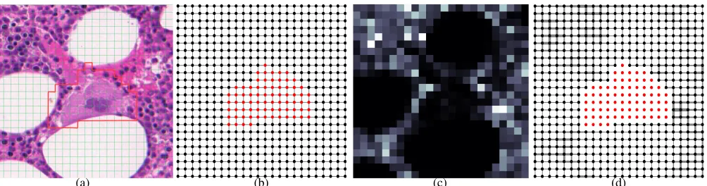
andj, according to a given criterion. Fig. 2 shows a sample
pathology image divided into 576 blocks in a 24× 24grid
and the corresponding 4-connected graph representing these blocks.
In this work, we employ the coding cost, cb ∈ [0,1], of
blockband its class,qb, as the metrics to define the similarity
between a pair of adjacent blocks, whereqb= 1if block b is
in the RoI and qb = 0 if is in the non-RoI. The coding cost
cb is computed as follows:
cb= HADb
HADmax, (5)
where HADb is the value of the Hadamard Transform of
blockb, which is calculated as the sum of absolute differences
between block b and its corresponding intra-predictions in
the horizontal and vertical directions [45]; and HADmax is
the maximum HAD value of all blocks in the image. The
Hadamard Transform is a fast and accurate way to estimate the coding cost of a block to be encoded using angular intra-prediction and is currently employed in the HEVC standard [11]. Note that according to Eq. 5, those blocks with the
smallest HAD values, i.e., those easy-to-code blocks, are
assigned the lowest coding cost, while those with the largest
HADvalues, i.e., those hard-to-code blocks, are assigned the
highest coding cost,cb= 1.
(a) (b) (c) (d)
Fig. 2: (a) Pathology image divided into24×24 = 576blocks. The RoI is delimited by the red contour. (b) Corresponding 4-connected
graph representing the RoI (red) and non-RoI (black) blocks. (c) Coding costs of blocks used to encode the G component, ranging from 0 (lowest cost - black ) to 1 (highest cost - white). (d) 4-connected graph with edges proportional to the corresponding weight ranging from small weights (thin lines) to large weights (thick lines).
via a thresholded Gaussian weighting function:
Wij =
1 2(e
−(1−ci
θ )
2+e−(1−cj
θ )
2), if iandj adjacent
andqi= 0,qj= 0
0, otherwise,
(6)
where θ is a parameter that determines the width of the
Gaussian weighting function. Fig. 2c shows the coding costs
of the24×24 = 576blocks used to encode the green color (G)
component of the pathology image depicted in Fig. 2a. Fig. 2d shows the corresponding 4-connected graph after computing the weight of edges according to Eq. 6. Note that the weight assignment of Eq. 6 disconnects the nodes representing the
RoI from those representing the non-RoI, as a weight = 0
effectively represents no connectivity. It is worth noticing two important aspects about the weight assignment in Eq. 6. First, an edge connecting two nodes representing low coding-cost blocks is assigned a small weight, while one connecting two nodes representing high coding-cost blocks is assigned a large weight. Second, within a region comprising blocks of similar coding costs, the edges connecting the corresponding nodes are assigned similar values. This is illustrated in Fig. 2d, where the dark regions in Fig. 2c have edges with small weights (i.e., thin lines) due to the low coding costs of the corresponding blocks. Moreover, these weights have similar values within these easy-to-code regions.
Let us now define the combinatorial Laplacian of graphG=
(V, E,A):
L=D−A, (7)
where the degree matrix, D, is a diagonal matrix whose ith
diagonal element,di, is equal to the sum of the weights of all
the edges incident to node i. Since L is a real, symmetric
matrix, it has a complete set of orthonormal eigenvectors with associated real, non-negative eigenvalues [46], [34]. The
spectral decomposition of the Laplacian is L = ΦΛΦT,
where Λ =diag(λ1, λ2, ..., λ|V|)is the diagonal matrix with
the eigenvalues ordered according to increasing magnitude
(0 = λ1 < λ2 ≤λ3 ≤...≤λ|V|) as diagonal elements and
Φ = (φ1|φ2|...|φ|V|) is the matrix with the correspondingly
ordered eigenvectors as columns [46], [34]. We can then define
a heat kernel by exponentiating the Laplacian matrix,L, with
timet:
Ht=e−tL=I−t
L+t
2
2!L
2−t 3
3!L
3+...., (8)
whereI is the |V| × |V| identity matrix. By substituting the
Laplacian in Eq. 8 by its eigenspectrumL= ΦΛΦT, the heat
kernel is expressed as:
Ht= Φe−tΛΦT. (9)
Eq. 9 is a graph kernel represented as a|V|×|V|symmetric
matrix [47], [48], in which the element for nodesi andj of
graphGis:
Ht(i, j) =
|V| X
k=1
e−λktφ
k(i)φk(j). (10)
Under the assumption that an amount ofheatisinjected at
a node i of the graph and is allowed to diffuse through the
edges, the heat kernel describes the flow of heat across the edges of the graph with time. In this work, we use such a heat
kernel todiffusea target bit budget across the edges of graph
Gso that each non-RoI node, or block, is assigned a portion
of that bit budget by considering their coding cost similarities with adjacent blocks and the overall structure of the graph. To
this end, we initially assign each non-RoI node b an amount
of heat energy equal toEbt=0:
Ebt=0=
( HADb P
|A|HADb, ifb∈A
0, otherwise, (11)
whereAis the set of non-RoI nodes adjacent to the RoI. We
then let the initial heat energy diffuse through the graph edges
as time t progresses until convergence, i.e., until the largest
difference between the heat energy accumulated by any
non-RoI node at time t and t−1 is ≤ dheat, where dheat is a
small constant. This results in a relatively smooth distribution of heat energy across the non-RoI nodes without incurring in large heat differences among adjacent non-RoI nodes.
After convergence of the diffusion process, we compute the
bit budget,Ωb, that is assigned to blockb:
Ωb =bΩnon−RoI×
|V| X
v=1
(a)t= 0 (b)t= 1 (c)t= 2 (d)t= 3
(e)t= 4 (f)t= 5 (g)t= 6 0
0.2 0.4 0.6 0.8 1 1.2 1.4 1.6 1.8 2
10-3
[image:6.612.55.563.55.324.2](h)t= 7
Fig. 3: (a)-(h) Heat energy accumulated by the blocks of the image in Fig. 2 as time progresses according to a diffusion process on the
corresponding graph. The amount of heat energy ranges from small (coldblocks - blue ) to large (hotblocks - yellow).
wherebxeis the nearest integer function onx,Ωnon−RoIis the
overall bit budget of the non-RoI, and Et
b =
P|V|
v=1Ht(v, b)
is the amount of heat energy accumulated by node b at time
t. The corresponding rate for blockbis then calculated as:
Rb= Ωb/Nb, (13)
whereNb is the number of pixels in the block. Based onRb,
the value of λ for block b can then be computed using the
model in Eq. 1. TheQP for block b is then computed using
the linear relationship in Eq. 2.
It is worth noticing that assigning the initial heat energy based on Eq. 11 allows for the encoding of the non-RoI with peripherally increasing quality around the RoI [8], [9]. In other words, the non-RoI blocks spatially close to the RoI are expected to be assigned a higher bit budget than that assigned to the non-RoI blocks spatially far from the RoI, particularly
for small values oft. Fig. 3 shows the heat energy accumulated
for non-RoI blocks as time progresses according to a diffusion
process on the graph depicted in Fig. 2d. At time t = 0, a
unit of heat energy is distributed among those non-RoI nodes surrounding the RoI according to their coding costs, while the
other non-RoI nodes are assigned zero heat. At t = 1, one
can observe that non-RoI blocks with low coding costs tend to accumulate relatively small amounts of heat energy. This is due to the weight assignment in Eq. 6, which prevents the
heat energy from flowing into easy-to-code regions. At t= 7,
however, the distribution of heat energy is relatively smooth across all non-RoI blocks according their distance to the RoI and coding costs.
B. Graph-based bit budget re-allocation
As explained in Section II, the actual number of bits used to encode each non-RoI block depends not only on the assigned
bit budget but also on the accuracy of the R-λmodel, i.e., on
the accuracy of parameters αand β in representing the R-D
characteristics of the non-RoI. To guarantee that the overall
bit budget, Ωnon−RoI, is respected and the target bit rate
is attained, our algorithm fine tunes the model’s parameters,
α and β, after each non-RoI block is encoded, as detailed
in Section II. However, despite this fine-tuning differences between the actual number of bits spent on each non-RoI
block, b, and the corresponding target bit budget, Ωb, may
still arise. To further guarantee that the overall target bit rate is accurately attained, we employ a graph-based approach to re-allocate any underspent or overspent bit budget of non-RoI
blockbto those uncoded non-RoI blocks adjacent tob. To this
end, we exploit the properties of the random walk matrix, P,
of the graph,G= (V, E,A), representing the blocks:
P=D−1A, (14)
where entrypi,j=pj,idescribes the probability of going from
nodeito nodej in one step of a Markov random walk on the
graph.
Matrix P provides information about how any underspent
or overspent bit budget can be re-allocated to those uncoded non-RoI blocks adjacent to the current non-RoI block. Since
matrix P is calculated using matrices D andA, it inherently
considers the coding costs similarities of blocks and the overall
structure of graphG.
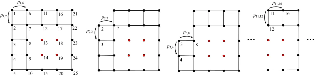
Let us consider an example 4-connected graph representing
an image divided into5×5 = 25blocks, as depicted in Fig. 4,
p1,6
p1,2
…
p2,7
p2,3 p3,8
p3,4
p11,16
p11,12
…
1 6
2 2
3 7
3
4 8
11
12 16
3
4
5 7
8
9
10 11
12
13
14
15 16
17
18
19
20 21
22
23
24
[image:7.612.53.555.61.181.2]25
Fig. 4:Sequential encoding of RoI and non-RoI blocks, represented as red and black nodes, respectively, of a graph. After encoding non-RoI
blockb, any underspent/overspent bit budget is re-allocated only to uncoded blocks adjacent tob, according to entries of the corresponding random walk matrix,P, which is updated by sequentially removing from the graph nodes representing coded blocks.
block b= 1. Let us denote the actual number of bits used to
encode non-RoI block b by Ωbb and the corresponding target
bit budget by Ωb. After encoding block b using Ωbb bits, the
associated heat energy, Ebbt, can be expressed as:
b
Ebt= Ωbb
Ωnon−RoI
. (15)
It then follows that ifΩbb 6= Ωb, thenEbbt6=Ebtdue to the linear
relationship in Eq. 15, where Ωnon−RoI is constant. In such
a case, it is important to guarantee that the total heat energy,
b
EGt, across all the nodes of the graph after encoding non-RoI
block b is always equal to the initial amount of heat energy
injected, EGt=0:
b
EGt =
|V| X
v=1
b
Evt =EGt=0= 1. (16)
Consequently, any overspending or underspending of Ωb
re-sults in an apparent change of Et
G [see Eq. 15]. In order to
respect the overall bit budget,Ωnon−RoI, Eq. 16 must be then
satisfied after encoding each non-RoI block.
Let us assume that the first non-RoI block of the example
in Fig. 4 is encoded using Ωb1 bits, where Ωb1 <Ω1. In other
words, the target bit budget of blockb= 1,Ω1, is underspent.
To satisfy Eq. 16, the unused bits Ωe1 = Ω1−Ωb1 should be
re-allocated among the uncoded (non-RoI) blocks adjacent to
blockb= 1based on the entries of matrixP. In this example,
the uncoded (non-RoI) blocks adjacent to block b = 1 are
blocksb= 2andb= 6(see Fig. 4). After re-allocatingΩe1, the
new bit budget of blockb= 2is thenΩ2= Ω2+ (Ωe1×p1,2).
Similarly, the new bit budget of block b = 6 is Ω6 = Ω6+
(Ωe1×p1,6), where p1,2+p1,6= 1 by definition of matrixP.
If block b= 2is the next non-RoI block to be encoded, any
bit budget difference, Ωe2, should be then re-allocated only to
its adjacent uncoded (non-RoI) blocks based on the entries of
matrix P, i.e., blocksb= 3 andb= 7, and not to blockb=
1, which has already been coded (see Fig. 4). Consequently,
matrixPshould be updated as blocks are sequentially encoded
so that any nodes representing coded blocks be sequentially
removed from G. This idea is illustrated in Fig. 4.
In general, any bit budget difference incurred after encoding
non-RoI block b, Ωb, is re-allocated to the bit budget of itse
adjacent uncoded blocks, represented by setJ, as follows:
Ωj=
max(σ·Ωj,Ωj−(pb,j· |Ωb|)),e if overspending
∀j∈J
min(ς·Ωj,Ωj+ (pb,j· |Ωb|)),e if underspending
,
(17)
whereσ= 0.95,ς = 1.05, pb,j is the {b, j} entry of matrix
P, andPjpb,j = 1. Note that if non-RoI block bis adjacent
to an uncoded RoI block j, probability pb,j is effectively 0
due to weight Wbj = 0, as defined by Eq. 6. Also note
that σ < 1 and ς > 1 guarantee that the bit budget Ωj
is not dramatically decreased if overspending or increased if
underspending, respectively. In cases whereΩbe is not fully
re-allocated among blocks in setJ, the bit budget re-allocation
in Eq. 17 is iteratively applied to uncoded blocks adjacent to
those in setJ until Eq. 16 is satisfied.
After encoding non-RoI block b and re-allocating any bit
budget difference, matrixPis re-calculated by removing from
Gthe node representing blockb. In other words, after encoding
block b, we compute the random walk matrix of graph G˜ =
( ˜V ,E), denoted by˜ P˜. The finite set of nodes,V˜ ⊆V, and the
corresponding set of edges,E˜ ⊆E, are computed as follows:
˜
V =V \Vencoded, (18a)
˜
E=E\Eencoded, (18b)
where Vencoded is the finite set of nodes of G representing
coded blocks and Eencoded is the corresponding set of edges
incident on them.
This clipping process, however, may result in blocks encoded at bit rates that greatly differ from their target bit rates, which inevitably results in overspending or underspending the overall bit budget. Our graph-based RC algorithm avoids this problem by distributing the overall bit budget according to the structure of the graph representing the coding cost similarities of blocks. Specifically, our graph-based bit budget allocation results in a smooth bit budget distribution, as exemplified in Fig. 3h. This bit budget distribution helps to minimize blocky artifacts by smoothly transitioning from high coding-cost regions to low coding-cost ones. Moreover, our graph-based bit budget re-allocation allows to re-allocate any bit budget differences to uncoded non-RoI blocks according to the structure of the graph, which also helps to minimize blocky artifacts. Our graph-based RC algorithm, therefore, requires no clipping of QPs to attain quality consistency in the non-RoI.
IV. EXPERIMENTAL EVALUATION
We implement our graph-based RC algorithm in the HEVC standard using the reference software HM16.9 [49]. HEVC is a block-based PTC standard for video compression that allows for the compression of individual images by using the intra-prediction coding mode, which can be employed in a lossless or a lossy fashion [27]. HEVC employs a tree structure to define the size of the constituent coding blocks (CBs) of the image. It employs the coding tree unit (CTU) as the basic unit, which consists of a luma coding tree block (CTB) and the corresponding chroma CTBs. For color images, one luma CB and two chroma CBs form a coding unit (CU) [11].
Current implementations of HEVC include an RC algorithm
based on an R-λmodel that takes into account the hierarchical
coding structure of the standard to distribute a bit budget to each coding level, i.e., Groups-Of-Picture (GOPs), pictures and CUs; and to compute the best set of QPs to attain a target bit rate [31]. Specifically, a QP is computed for each largest CU (LCU). This RC algorithm also updates the model’s
parameters,αandβ, as pictures and LCUs are encoded when
using inter-prediction. Unfortunately, for the case of encoding of a single image using intra-prediction, the algorithm does not update the model’s parameters after encoding each LCU, which usually results in large discrepancies between the target
and actual bit rates if α and β do not accurately reflect the
R-D characteristics of the image [15]. We evaluate four distinct approaches:
1) the current RC algorithm available in the HM reference
software whenαandβ are computeda priorifor each
test image;
2) the current RC algorithm available in the HM reference
software whenαandβare computeda priorifor a large
set of training images;
3) the RC algorithm proposed in [15] for HEVC, which
is based on an R-λ model and updates the model’s
parameters after encoding each LCU; and 4) our proposed graph-based RC algorithm.
It is important to note that approaches 1 and 2 do not update
the model’s parameters, α and β, after encoding each LCU.
However, approach 1 is expected to attain the target bit rate
most accurately, as the model’s parameters used by this ap-proach for each image are computed using the same image as training data. For this reason, approach 1 is used as a baseline. It should also be noted that approach 1 requires compressing
each test image, a priori, at a wide range of bit rates in
order to determine their specific R-D characteristics and the corresponding model’s parameters, which is not practical.
The accuracy of all evaluated approaches is computed in terms of the bit-rate error (BRE), which measures how accu-rately the target bit rate is attained; negative numbers indicate
underspending Ωnon−RoI, while positive numbers indicates
overspendingΩnon−RoI.
A wide range of pathology images with a single or multiple RoIs are evaluated, as tabulated in the first three columns of Tables I and II. These images are available through the Center for Biomedical Informatics and Information Technology of the US National Cancer Institute [50]. The test images are compressed using intra-prediction as a single RGB frame in
4:4:4 format with an LCU size of 64×64 samples. The
HM reference software is modified in order to allow for lossless RoI coding in approaches 1 and 2. This is done by feeding residual blocks depicting the RoI directly to the entropy coder and by-passing any processing that affects the perfect reconstruction of these blocks. The LCUs representing the RoIs and the non-RoI are signalled to the encoder and
decoder by a binary mask, which is computed a priori by
manually delineating the RoIs. Any LCU that contains RoI pixels is considered as part of the RoI. A variety of target bit rates, expressed in terms of bits per pixel per component (bpppc), is used to compress the non-RoI of each of these test images, ranging from 0.067 bpppc to 2.0 bpppc. All images are 8 bpppc.
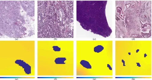
Fig. 5 depicts four of the test images and the corresponding heat energy accumulated by each of the constituent blocks after convergence of the diffusion process. It can be seen that our graph-based RC algorithm distributes the heat en-ergy smoothly across all non-RoI blocks even when multiple RoIs are defined. Note that image LYMP3 includes sections depicting no tissue. In this case, the diffusion process prevents the corresponding blocks from accumulating a large amount of energy, since these smooth white sections are very easy to encode. This is evident in the lower left corner of Fig. 5g.
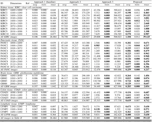
Average absolute BRE values of all evaluated approaches are tabulated in Tables I and II, along with the maximum and minimum absolute BRE values attained in each case, and the values attained per tissue type and for all tissue types. The last row of Table II also tabulates results for all the test images. Approach 1 attains the best performance, with average absolute BRE values very close to zero for all tissue types. Let us recall that approach 1 is the baseline approach and is evaluated only to show the accuracy of the current RC algorithm in HEVC when the appropriate model’s parameters are used. Since this approach requires computing
these parameters a priori, its applicability is very limited.
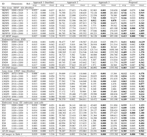
TABLE I: Characteristics of SKNF, END, LNGF, and ES images, and absolute BRE values (%) of all approaches
ID Dimensions RoI Approach 1 (baseline) Approach 2 Approach 3 Proposed
avg min max avg min max avg min max avg min max
Skin tissue. SKNF: skin fibroblast
SKNF1 3200×2816 5 0.022 0.000 0.037 88.513 27.653 176.450 92.903 0.001 310.658 0.945 0.079 1.344
SKNF2 4096×3328 3 0.110 0.000 3.216 74.390 22.272 140.645 74.128 0.000 281.883 0.726 0.276 0.919
SKNF3 1600×2560 1 0.021 0.000 0.057 69.501 22.090 124.974 22.558 0.025 78.589 0.695 0.222 7.981
SKNF4 1280×4160 2 0.013 0.001 0.035 101.530 27.134 160.933 7.508 0.000 92.677 0.166 0.010 0.932
SKNF5 3328×3072 2 0.011 0.001 0.042 89.936 32.508 186.243 0.012 0.001 0.078 0.051 0.003 0.329
SKNF6 4160×1280 3 0.033 0.003 0.099 56.741 12.428 107.813 0.758 0.000 16.673 0.151 0.075 0.342
SKNF7 4096×3200 4 0.015 0.003 0.026 73.022 18.520 143.394 3.773 0.003 39.542 0.346 0.014 0.581
SKNF8 1920×2880 1 0.013 0.000 0.092 79.595 17.754 124.812 52.571 0.001 493.100 0.368 0.000 4.735
SKNF9 3392×2280 4 0.019 0.003 0.042 75.718 24.395 157.961 37.846 0.002 274.435 0.197 0.015 1.059
SKNF10 3520×2880 1 0.013 0.000 0.039 86.785 30.786 195.552 69.223 0.001 230.169 0.483 0.001 4.009
All SKNF images 0.027 0.000 3.216 79.573 12.428 195.552 36.128 0.000 493.100 0.413 0.000 7.981
Endometrial tissue. END
END1 2880×3200 4 0.016 0.001 0.050 58.477 7.397 130.567 25.418 0.025 190.371 0.411 0.022 -0.229
END2 3200×2816 3 0.015 0.001 0.042 63.827 5.810 166.758 26.910 0.003 211.514 0.532 0.062 1.920
END3 3072×2112 3 0.023 0.000 0.078 104.654 38.330 228.439 5.004 0.001 30.545 0.381 0.015 0.755
END4 3072×1920 2 0.010 0.000 0.037 102.863 40.558 218.528 125.714 0.006 1050.340 0.731 0.286 2.202
END5 4096×2368 1 0.036 0.002 0.084 100.585 33.183 234.546 149.344 0.002 1353.582 0.409 0.159 1.370
END6 2280×2112 2 0.016 0.003 0.032 36.723 5.582 72.883 48.888 0.003 294.768 0.289 0.059 1.370
END7 1280×4096 2 0.017 0.001 0.039 43.772 5.700 90.470 60.552 0.012 814.534 0.521 0.077 1.829
END8 2112×2816 4 0.014 0.000 0.046 67.466 8.905 112.454 9.307 0.001 133.010 0.327 0.007 1.211
END9 2816×3200 2 0.015 0.001 0.031 69.745 22.168 143.642 7.812 0.003 111.774 0.155 0.007 0.362
END10 3200×2880 1 0.017 0.000 0.050 92.653 37.843 191.037 1.971 0.000 28.569 0.279 0.087 0.754
All END images 0.018 0.000 0.084 74.076 5.582 234.546 46.092 0.000 1353.582 0.403 0.007 2.202
Lung tissue. LNGF: lung fibroblast
LNGF1 3072×3840 2 0.006 0.001 0.017 59.009 17.330 118.868 4.453 0.001 13.384 0.112 0.042 0.378
LNGF2 3840×1920 5 0.017 0.000 0.054 72.731 14.143 154.644 39.825 0.031 193.198 0.834 0.351 1.720
LNGF3 3520×2880 1 0.010 0.000 0.027 98.892 33.136 204.011 27.781 0.000 151.635 0.291 0.020 0.645
LNGF4 2816×4800 5 0.007 0.000 0.014 57.582 7.736 144.040 0.186 0.000 4.840 0.063 0.006 0.221
LNGF5 2816×2560 1 0.013 0.000 0.027 30.549 0.892 78.859 0.155 0.000 4.476 0.018 0.003 0.077
LNGF6 3392×2560 2 0.010 0.000 0.019 50.959 3.664 107.008 0.192 0.000 2.620 0.182 0.016 0.382
LNGF7 2816×2560 1 0.016 0.002 0.032 44.441 5.270 82.741 0.240 0.000 2.684 0.099 0.001 0.251
LNGF8 1600×3328 3 0.017 0.000 0.076 37.172 7.472 70.989 1.369 0.000 35.469 0.062 0.011 0.262
LNGF9 3200×3520 3 0.014 0.000 0.031 75.723 29.400 173.309 29.990 0.005 180.836 0.157 0.029 0.614
LNGF10 4096×1600 1 0.018 0.000 0.080 58.640 11.305 103.275 0.530 0.000 15.198 0.069 0.001 1.720
All LNGF images 0.013 0.000 0.080 58.570 0.892 204.011 10.472 0.000 193.198 0.189 0.001 1.720
Embryonic tissue. ES: embryonic stem cells
ES1 3200×2880 2 0.018 0.000 0.051 84.481 36.141 160.161 45.602 0.002 211.894 0.555 0.115 1.153
ES2 3328×4096 3 0.011 0.001 0.024 81.619 24.380 150.337 67.626 0.004 188.937 0.600 0.008 0.870
ES3 3328×3328 3 0.014 0.000 0.053 106.543 41.747 225.338 29.127 0.001 520.424 0.823 0.190 2.387
ES4 4480×3200 6 0.075 0.000 2.102 106.302 41.151 213.199 24.751 0.000 277.427 0.643 0.000 1.180
ES5 3200×3200 1 0.018 0.000 0.091 59.765 23.418 131.989 31.364 0.001 109.611 0.501 0.079 1.601
ES6 2560×2816 4 0.014 0.000 0.080 75.480 33.913 148.534 16.288 0.000 128.471 0.508 0.006 0.989
ES7 3520×4096 5 0.028 0.001 0.071 62.670 22.782 119.238 1.208 0.000 16.403 0.070 0.004 0.292
ES8 4480×4480 2 0.003 0.001 0.008 60.994 20.765 113.633 4.381 0.000 30.130 0.111 0.045 0.404
ES9 4160×4160 5 0.003 0.000 0.016 75.899 29.067 131.535 2.007 0.000 22.876 0.104 0.005 0.355
ES10 5120×4480 3 0.006 0.000 0.028 66.311 23.558 132.134 2.651 0.000 42.384 0.054 0.010 0.222
All ES images 0.020 0.000 0.271 78.287 29.223 153.063 23.191 0.001 157.787 0.385 0.051 0.941
All images in Table I 0.019 0.000 3.216 72.627 0.892 234.546 28.971 0.000 1353.582 0.347 0.000 7.981
Best results among approaches 2, 3 and the proposed algorithm are highlighted in bold font.
whole image, i.e., non-RoI and RoIs, it is evident that when used to compress only the non-RoI, these parameters do not accurately represent the R-D characteristics of this region. As a consequence, approach 1 tends to perform poorly for this image at this very low target bit rate.
As expected, approach 2 attains the worst performance across all tissue types since this approach does not update the model’s parameters after encoding each LCU. Consequently, if these parameters do not accurately reflect the R-D charac-teristics of the non-RoI, this approach fails to compute the appropriate set of QPs needed to attain the target bit rate.
Approach 3 performs better than approach 2 since the model’s parameters are updated after encoding each LCU. This approach can also attain minimum absolute BRE values very close to zero for some of the target bit rates, as tabulated in the
corresponding columns labeled min. However, it still attains
TABLE II: Characteristics of KIRC, PANC, GBM, COAD, and LYMP images, and absolute BRE values (%) of all approaches
ID Dimensions RoI Approach 1 (baseline) Approach 2 Approach 3 Proposed
avg min max avg min max avg min max avg min max
Kidney tissue. KIRC: clear cell carcinoma
KIRC1 4480×3200 3 0.008 0.000 0.045 110.100 30.893 220.927 42.256 0.001 390.622 0.241 0.056 1.299
KIRC2 4160×4480 2 0.018 0.002 0.036 86.347 26.181 175.229 5.312 0.003 88.297 0.198 0.012 0.403
KIRC3 1600×3328 3 0.014 0.001 0.038 48.807 3.195 124.374 89.602 0.088 568.023 6.613 1.443 39.125
KIRC4 3520×2880 1 0.891 0.001 26.464 97.763 33.758 218.182 32.788 0.005 291.756 0.821 0.123 3.081
KIRC5 1600×1920 3 0.023 0.000 0.103 52.562 1.984 138.571 90.502 0.019 257.921 0.341 0.012 1.712
KIRC6 2816×1920 2 0.022 0.000 0.068 49.205 7.808 105.949 9.651 0.002 108.634 0.680 0.217 2.668
KIRC7 3072×2880 1 0.017 0.000 0.040 57.522 0.975 140.611 11.817 0.000 96.679 0.722 0.060 2.527
KIRC8 2560×2816 4 0.022 0.001 0.085 60.108 0.089 159.384 0.847 0.000 15.097 0.238 0.028 1.008
KIRC9 2816×4096 3 0.010 0.000 0.023 85.706 20.490 191.507 5.678 0.008 67.909 0.615 0.021 1.108
KIRC10 1280×3200 1 0.036 0.002 0.077 59.377 14.684 122.057 7.629 0.008 194.585 0.570 0.244 0.987
All KIRC images 0.106 0.000 26.464 70.750 0.089 220.927 29.608 0.000 568.023 1.104 0.012 39.125
Pancreatic tissue. PANC
PANC1 4800×3200 1 0.007 0.000 0.039 67.425 18.349 143.388 2.546 0.002 18.398 0.202 0.043 0.671
PANC2 1600×2560 2 0.011 0.001 0.052 45.144 9.217 91.600 0.985 0.061 17.828 1.336 0.044 4.217
PANC3 3328×3072 1 0.009 0.000 0.020 78.221 25.212 184.838 0.572 0.001 9.334 0.225 0.023 0.565
PANC4 2816×3200 3 0.026 0.005 0.039 46.819 0.650 107.293 1.269 0.001 15.001 0.086 0.001 0.479
PANC5 1920×2880 2 0.025 0.001 0.116 37.998 2.249 80.314 3.494 0.002 10.669 0.223 0.005 0.962
PANC6 2240×4096 4 0.007 0.000 0.039 78.399 22.327 166.724 11.408 0.000 64.197 0.221 0.036 0.968
PANC7 3328×3072 1 0.013 0.001 0.021 84.014 21.676 203.571 102.393 0.009 889.886 0.126 0.000 0.692
PANC8 3520×2560 3 0.010 0.000 0.024 27.679 0.045 79.809 0.535 0.000 6.980 0.056 0.001 0.439
PANC9 2112×2816 1 0.010 0.000 0.037 82.975 8.342 166.817 1.114 0.001 11.215 0.077 0.000 0.396
PANC10 3072×2816 1 0.013 0.001 0.019 84.792 26.466 233.912 0.448 0.003 9.228 0.037 0.000 0.306
All PANC images 0.013 0.000 0.116 63.347 0.045 233.912 12.476 0.000 889.886 0.259 0.000 4.217
Brain tissue. GBM: glioblastoma multiforme
GBM1 4480×3840 3 0.735 0.004 1.824 78.673 2.019 298.189 6.675 0.016 42.022 0.264 0.142 1.456
GBM2 3392×3072 1 0.006 0.000 0.033 46.117 0.186 144.933 19.984 0.000 137.293 0.015 0.000 0.074
GBM3 3520×2880 2 0.028 0.005 0.037 84.557 23.363 220.511 110.748 1.963 427.996 0.724 0.383 2.054
GBM4 2880×2816 4 0.017 0.002 0.035 123.321 33.411 319.569 0.390 0.000 5.800 0.129 0.010 0.647
All GBM images 0.197 0.000 1.842 83.167 0.186 319.569 34.449 0.000 427.996 0.283 0.000 2.054
Colon tissue. COAD: colon adenocarcinoma
COAD1 4096×3840 2 0.003 0.000 0.014 54.157 13.098 122.594 41.432 0.000 177.730 0.154 0.041 0.687
COAD2 2816×4480 3 0.010 0.004 0.019 52.397 0.077 134.907 1.936 0.001 9.374 1.611 0.089 4.712
COAD3 3840×3200 2 0.013 0.001 0.053 40.036 0.003 116.890 2.572 0.000 15.764 0.093 0.007 0.840
All COAD images 0.009 0.000 0.053 48.863 0.003 134.907 15.313 0.000 177.730 0.619 0.007 4.712
Lymphatic tissue. LYMP: lymphoma
LYMP1 1280×1280 1 0.042 0.001 0.097 36.771 1.627 78.672 9.374 0.004 87.621 0.673 0.281 5.630
LYMP2 1920×3840 2 0.047 0.002 0.084 27.684 0.045 139.748 0.128 0.001 1.322 0.166 0.009 0.571
LYMP3 4480×4480 3 0.064 0.000 0.364 40.198 0.256 131.634 19.990 0.000 162.425 0.361 0.020 2.293
All LYPM images 0.051 0.000 0.364 34.884 0.045 139.748 9.831 0.000 162.425 0.400 0.020 5.630
All images in Table II 0.080 0.000 26.464 61.960 0.003 319.569 21.881 0.000 889.886 0.533 0.000 39.125
All images in Tables I and II 0.050 0.000 26.464 70.124 0.003 319.569 22.536 0.000 1353.582 0.459 0.000 39.125
Best results among approaches 2, 3 and the proposed algorithm are highlighted in bold font.
of adjacent blocks [15]. Consequently, approach 3 can easily fail if the model’s parameters or the bit budget allocation is inaccurate. Note however that for some of the test images; i.e., SKNF5, LYMP2 and PANC2, approach 3 attains a very good performance. This indicates that the updating process results in a set of model’s parameters that accurately represent the R-D characteristics of the non-RoI of these images.
Our proposed graph-based RC algorithm attains a consistent performance for all tissue types with the lowest average absolute BRE values. Specifically, the average absolute BRE value attained by our algorithm for all test images is 0.459%, which is much lower than that attained by Approach 3 (22.536 %) and Approach 2 (70.124 %). The minimum and maximum absolute BRE values attained by our algorithm are also very close to zero for all of the test images. Note that for image KIRK3, the maximum absolute BRE values attained by our algorithm and approach 3 are 39.13% and 568.02%,
respectively, which are attained at very low bit rates (<0.133
bpppc). These very high absolute BRE values can be explained
by the fact that although both approaches update the model’s parameters after encoding each LCU, the limited range of QP values available in HEVC makes it very challenging to accurately attain very low target bit rates for each LCU if the initial model’s parameters are very different from those that accurately describe the R-D characteristics of the non-RoI. However, note that our algorithm still attains the lowest average absolute BRE for this image.
(a) (b) (c) (d)
[image:11.612.57.562.54.323.2](e) (f) (g) (h)
Fig. 5:Four test images and the corresponding heat energy accumulated by each of the constituent blocks after convergence of the diffusion
process: (a),(e) GBM2; (b),(f) COAD3; (c),(g) LYMP3; and (d),(h) SKNF1. The amount of heat energy is depicted by a distinct color ranging from blue (coldblocks) to yellow (hotblocks). Blue blocks represent the RoI.
defined, like in the case of image END1, non-RoI blocks are likely to be surrounded by multiple RoI blocks, which may prevent the clipping process from having enough QPs to compute an accurate narrow range to clip the current QP. This inevitably results in inaccurately attaining the overall target bit rate. Our graph-based RC algorithm, on the other hand, assigns each non-RoI block a bit budget based on their coding costs similarities with adjacent blocks. These similarities are
represented by the structure of the graph, G, representing
the blocks. Therefore, when multiple RoIs are defined, the QP selection of a block only depends on the corresponding assigned bit budget. Moreover, any bit budget differences are re-allocated among uncoded blocks based on the structure of
the same graph,G, which guarantees that the target bit rate is
accurately attained.
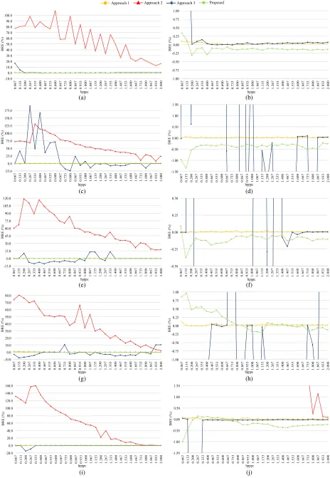
Our graph-based RC algorithm consistently attains very low BRE values across all target bit rates and images plotted in Fig. 6. For image END1, which depicts four RoIs, our algorithm attains BRE values very close to zero, with a maximum absolute BRE value of only 1.375% (see Fig. 6d).
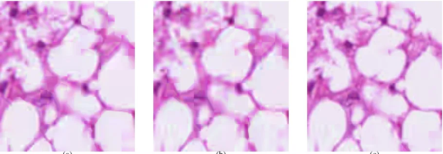
Fig. 7 shows a reconstructed section of the non-RoI of image LYMP2 encoded at the very low target bit rate of 0.133 bpppc, which is a low target bit rate at which the BRE values attained by our graph-based RC algorithm and those attained by approach 1 and approach 3 are the most similar. Note that our algorithm produces less blocky artifacts thanks to the graph-based bit budget allocation and re-allocation processes, both of which take into account the coding cost similarities of blocks. Blocky artifacts are more evident in the images
reconstructed by approaches 1 (BRE=−0.005%) and 3 (BRE
=−0.006%), despite the fact that their BRE values are closer
to zero than that of our algorithm (BRE =−0.439%). These
evident blocky artifacts are mainly due to the bit budget as-signment, which does not consider the coding cost similarities of adjacent blocks, therefore resulting in adjacent blocks being compressed at very different qualities despite the clipping process used to attain quality consistency. The Peak Signal-to-Noise Ratio (PSNR) values attained at this low target bit rate
for the {R, G, B} color components of the non-RoI of this
image are {28.71,27.62,28.57}dB, {28.44,27.73,28.50}dB,
and{28.55,27.99,28.60}dB for approach 1, approach 3 and
our algorithm, respectively.
A. Applicability to other medical images
The proposed graph-based RC algorithm is suitable for other medical images. However, it is particularly useful for coding very large medical images, such as pathology images. As previously discussed, when the number of blocks needed to encode an image is very large, RC tends to perform very poorly if there is no mechanism to compensate for the inaccuracies incurred after encoding each block, since the individual inaccuracies tend to amount to a large value.
We have tested our algorithm in other medical images. Specifically, 20 MRI and CT slices, with sizes ranging from
256× 256 to 1024 × 1024 pixels and up to three RoIs.
Approach 1 Approach 2 Approach 3 Proposed -10.0 0.0 10.0 20.0 30.0 40.0 50.0 60.0 70.0 80.0 90.0 100.0 2. 000 1. 933 1. 867 1. 800 1. 733 1. 667 1. 600 1. 533 1. 467 1. 400 1. 333 1. 267 1. 200 1. 133 1. 067 1. 000 0. 933 0. 867 0. 800 0. 733 0. 667 0. 600 0. 533 0. 467 0. 400 0. 333 0. 267 0. 200 0. 133 0. 067 BRE ( % ) bpppc (a) -1.00 -0.75 -0.50 -0.25 0.00 0.25 0.50 0.75 1.00 2. 000 1. 933 1. 867 1. 800 1. 733 1. 667 1. 600 1. 533 1. 467 1. 400 1. 333 1. 267 1. 200 1. 133 1. 067 1. 000 0. 933 0. 867 0. 800 0. 733 0. 667 0. 600 0. 533 0. 467 0. 400 0. 333 0. 267 0. 200 0. 133 0. 067 BRE ( % ) bpppc (b) -25.0 0.0 25.0 50.0 75.0 100.0 125.0 150.0 175.0 2. 000 1. 933 1. 867 1. 800 1. 733 1. 667 1. 600 1. 533 1. 467 1. 400 1. 333 1. 267 1. 200 1. 133 1. 067 1. 000 0. 933 0. 867 0. 800 0. 733 0. 667 0. 600 0. 533 0. 467 0. 400 0. 333 0. 267 0. 200 0. 133 0. 067 BRE ( % ) bpppc (c) -1.50 -1.00 -0.50 0.00 0.50 1.00 1.50 2. 000 1. 933 1. 867 1. 800 1. 733 1. 667 1. 600 1. 533 1. 467 1. 400 1. 333 1. 267 1. 200 1. 133 1. 067 1. 000 0. 933 0. 867 0. 800 0. 733 0. 667 0. 600 0. 533 0. 467 0. 400 0. 333 0. 267 0. 200 0. 133 0. 067 BRE ( % ) bpppc (d) -15.0 0.0 15.0 30.0 45.0 60.0 75.0 90.0 105.0 120.0 2. 000 1. 933 1. 867 1. 800 1. 733 1. 667 1. 600 1. 533 1. 467 1. 400 1. 333 1. 267 1. 200 1. 133 1. 067 1. 000 0. 933 0. 867 0. 800 0. 733 0. 667 0. 600 0. 533 0. 467 0. 400 0. 333 0. 267 0. 200 0. 133 0. 067 BRE ( % ) bpppc (e) -0.50 -0.25 0.00 0.25 0.50 2. 000 1. 933 1. 867 1. 800 1. 733 1. 667 1. 600 1. 533 1. 467 1. 400 1. 333 1. 267 1. 200 1. 133 1. 067 1. 000 0. 933 0. 867 0. 800 0. 733 0. 667 0. 600 0. 533 0. 467 0. 400 0. 333 0. 267 0. 200 0. 133 0. 067 BRE ( % ) bpppc (f) -10.0 0.0 10.0 20.0 30.0 40.0 50.0 60.0 70.0 80.0 2. 000 1. 933 1. 867 1. 800 1. 733 1. 667 1. 600 1. 533 1. 467 1. 400 1. 333 1. 267 1. 200 1. 133 1. 067 1. 000 0. 933 0. 867 0. 800 0. 733 0. 667 0. 600 0. 533 0. 467 0. 400 0. 333 0. 267 0. 200 0. 133 0. 067 BRE ( % ) bpppc (g) -1.00 -0.75 -0.50 -0.25 0.00 0.25 0.50 0.75 1.00 2. 000 1. 933 1. 867 1. 800 1. 733 1. 667 1. 600 1. 533 1. 467 1. 400 1. 333 1. 267 1. 200 1. 133 1. 067 1. 000 0. 933 0. 867 0. 800 0. 733 0. 667 0. 600 0. 533 0. 467 0. 400 0. 333 0. 267 0. 200 0. 133 0. 067 BRE ( % ) bpppc (h) -20.0 0.0 20.0 40.0 60.0 80.0 100.0 120.0 140.0 160.0 2. 000 1. 933 1. 867 1. 800 1. 733 1. 667 1. 600 1. 533 1. 467 1. 400 1. 333 1. 267 1. 200 1. 133 1. 067 1. 000 0. 933 0. 867 0. 800 0. 733 0. 667 0. 600 0. 533 0. 467 0. 400 0. 333 0. 267 0. 200 0. 133 0. 067 BRE ( % ) bpppc (i) -1.50 -1.00 -0.50 0.00 0.50 1.00 1.50 2. 000 1. 933 1. 867 1. 800 1. 733 1. 667 1. 600 1. 533 1. 467 1. 400 1. 333 1. 267 1. 200 1. 133 1. 067 1. 000 0. 933 0. 867 0. 800 0. 733 0. 667 0. 600 0. 533 0. 467 0. 400 0. 333 0. 267 0. 200 0. 133 0. 067 BRE ( % ) bpppc (j)
Fig. 6: BRE values (%) of the evaluated approaches for various bit rates (bpppc). (a),(b) SKNF6; (c),(d) END1; (e),(f) LNGF1; (g),(h)
(a) (b) (c)
Fig. 7: Reconstructed non-RoI section of test image LYMP2 encoded at 0.133 bpppc using (a) approach 1, (b) approach 3, and (c) the proposed graph-based RC algorithm.
inaccuracies in attaining the target bit rate of each block do not amount to a large value.
B. Implementation details
This section discusses the numerical implementation of our graph-based bit budget allocation. The heat kernel in Eq. 8 requires computing the complete eigenspectrum of the
Laplacian matrix,L, which may be computationally expensive
for very large graphs. For example, the graph for test image
ES10 comprises 80×70 = 5600 nodes, when blocks of
64×64 samples are used. However, the Laplacian matrices of the graphs of all test images are symmetric, positive-definite, and very sparse. We take advantage of this fact to reduce the computational complexity by using the Krylov subspace projection technique [51], which is an iterative method for sparse matrix problems. This particular technique allows to
approximateetA=e−tLby an element of the Krylov subspace
κm ≡span{tA,(tA)2, ...,(tA)m−1)}, where m |L|. The
heat kernel in Eq. 8 is then computed using the following approximation:
e−tL≈ VmetHmτ
1, (19)
where Vm are the orthonormal basis of the Krylov subspace
κm, Hm is the upper Hessenberg matrix resulting from the
Arnoldi process, and τ1 is the first column of the identity
matrix Im.
V. CONCLUSION
This paper presented a new graph-based RC algorithm for RoI coding in pathology imaging within the context of block-based PTC. The algorithm encodes the non-RoI in a lossy manner at a specific target bit rate and the RoI in a lossless manner. It employs a graph to represent the coding cost similarities of the constituent blocks of the image. Based on the structure of such graph, the algorithm distributes a target bit budget among the non-RoI blocks using a graph kernel. The target bit rate of the non-RoI is accurately attained by
employing an R-λmodel to sequentially approximate the
R-D characteristics of the non-RoI as the constituent blocks are encoded. The structure of the graph is also exploited to
guarantee that the target bit budget is respected by re-allocating any bit budget differences incurred after encoding each non-RoI block. The proposed algorithm is implemented in HEVC and compared to other RC algorithms designed to encode single images using block-based PTC with lossless RoI coding capabilities. Evaluations over a large variety of pathology images with multiple RoIs show that the proposed algorithm is capable of attaining the target bit rate very accurately while minimizing blocky artifacts in the reconstructed non-RoI.
REFERENCES
[1] A. Madabhushi, “Digital pathology image analysis: opportunities and
challenges,”Imaging in Medicine, pp. 7–10, 2009.
[2] M. May, “A better lens on disease.”Scientific American, vol. 302, no. 5,
pp. 74–77, 2010.
[3] D. Racoceanu, D. Ameisen, A. Veillard, B. B. Cheikh, E. Attieh,
P. Brezillon, J.-B. Yun`es, J.-M. Temerson, L. Toubiana, V. Vergeret al.,
“Towards efficient collaborative digital pathology: a pioneer initiative of
the flexmim project,”Diagnostic Pathology, vol. 1, no. 8, 2016.
[4] C. Bernard, S. Chandrakanth, I. S. Cornell, J. Dalton, A. Evans, B. M. Garcia, C. Godin, M. Godlewski, G. H. Jansen, A. Kabani
et al., “Guidelines from the canadian association of pathologists for establishing a telepathology service for anatomic pathology using
whole-slide imaging,”Journal of Pathology Informatics, vol. 5, 2014.
[5] M. Sahota, B. Leung, S. Dowdell, and G. M. Velan, “Learning pathology using collaborative vs. individual annotation of whole slide images: a
mixed methods trial,”BMC Medical Education, vol. 16, no. 1, p. 311,
2016.
[6] T.-H. Song, V. Sanchez, H. ElDaly, and N. Rajpoot, “Dual-channel active contour model for megakaryocytic cell segmentation in bone
marrow trephine histology images,”IEEE Transactions on Biomedical
Engineering, 2017.
[7] V. Sanchez, “Joint source/channel coding for prioritized wireless trans-mission of multiple 3-D regions of interest in 3-D medical imaging
data,” IEEE Transactions on Biomedical Engineering, vol. 60, no. 2,
pp. 397–405, 2013.
[8] V. Sanchez, R. Abugharbieh, and P. Nasiopoulos, “3-D scalable medical
image compression with optimized volume of interest coding,” IEEE
Transactions on Medical Imaging, vol. 29, no. 10, pp. 1808–1820, 2010. [9] K. Krishnan, M. W. Marcellin, A. Bilgin, and M. S. Nadar, “Efficient
transmission of compressed data for remote volume visualization,”IEEE
Transactions on Medical Imaging, vol. 25, no. 9, pp. 1189–1199, 2006. [10] T. Wiegand, G. J. Sullivan, G. Bjontegaard, and A. Luthra, “Overview of
the H. 264/AVC video coding standard,”IEEE Transactions on Circuits
and Systems for Video Technology, vol. 13, no. 7, pp. 560–576, 2003. [11] G. J. Sullivan, J. Ohm, W.-J. Han, and T. Wiegand, “Overview of the
high efficiency video coding (HEVC) standard,”IEEE Transactions on
[12] V. Sanchez, F. Auli-Llinas, J. Bartrina-Rapesta, and J. Serra-Sagrista, “HEVC-based lossless compression of Whole Slide pathology images,” in2014 IEEE Global Conference on Signal and Information Processing (GlobalSIP), Dec 2014, pp. 297–301.
[13] H. Chen, G. Braeckman, S. M. Satti, P. Schelkens, and A. Munteanu, “HEVC-based video coding with lossless region of interest for
telemedicine applications,” in20th International Conference on Systems,
Signals and Image Processing (IWSSIP). IEEE, 2013, pp. 129–132. [14] V. Sanchez, F. Auli-Llinas, J. Bartrina-Rapesta, and J. Serra-Sagrista,
“Improvements to HEVC Intra Coding for Lossless Medical Image
Compression,” in2014 Data Compression Conference, March 2014, pp.
423–423.
[15] V. Sanchez, F. Auli-Llinas, R. Vanam, and J. Bartrina-Rapesta, “Rate control for lossless region of interest coding in HEVC intra-coding with
applications to digital pathology images,” in2015 IEEE International
Conference on Acoustics, Speech and Signal Processing (ICASSP), April 2015, pp. 1250–1254.
[16] J.-H. Lee and C. Yoo, “Scalable roi algorithm for h. 264/svc-based video
streaming,”IEEE Transactions on Consumer Electronics, vol. 57, no. 2,
2011.
[17] M. Meddeb, M. Cagnazzo, and B. Pesquet-Popescu,
“Region-of-interest-based rate control scheme for high-efficiency video coding,”APSIPA
Transactions on Signal and Information Processing, vol. 3, 2014. [18] Z. Chen and C. Guillemot, “Perceptually-friendly H.264/AVC video
coding based on foveated just-noticeable-distortion model,”IEEE
Trans-actions on Circuits and Systems for Video Technology, vol. 20, no. 6, pp. 806–819, 2010.
[19] H. Meuel, M. Munderloh, F. Kluger, and J. Ostermann, “Codec indepen-dent region of interest video coding using a joint pre-and postprocessing
framework,” in2016 IEEE International Conference on Multimedia and
Expo (ICME). IEEE, 2016, pp. 1–6.
[20] K. Perez-Daniel and V. Sanchez, “Luma-aware Multi-model Rate-control
for HDR Content in HEVC,” in2017 IEEE International Conference on
Image Processing (ICIP), September 2017, pp. 1022–1026.
[21] M. Zhou, H.-M. Hu, and Y. Zhang, “Region-based intra-frame
rate-control scheme for high efficiency video coding,” inIEEE 2014 Annual
Summit and Conference, Asia-Pacific Signal and Information Processing Association (APSIPA), 2014, pp. 1–4.
[22] M. Xu, X. Deng, S. Li, and Z. Wang, “Region-of-interest based con-versational HEVC coding with hierarchical perception model of face,”
IEEE Journal of Selected Topics in Signal Processing, vol. 8, no. 3, pp. 475–489, 2014.
[23] W. Zhao, J. Fu, Y. Lu, S. Li, and D. Zhao, “Region-of-interest based
coding scheme for synthesized video,” inIEEE 2015 Visual
Communi-cations and Image Processing (VCIP). IEEE, 2015, pp. 1–4. [24] M. Wang, K. N. Ngan, and H. Li, “Low-delay rate control for consistent
quality using distortion-based lagrange multiplier,”IEEE Transactions
on Image Processing, vol. 25, no. 7, pp. 2943–2955, 2016.
[25] M. Zhou, Y. Zhang, B. Li, and H.-M. Hu, “Complexity-based intra frame rate control by jointing inter-frame correlation for high efficiency video
coding,”Journal of Visual Communication and Image Representation,
2016.
[26] S. Li, M. Xu, Z. Wang, and X. Sun, “Optimal Bit Allocation for CTU
Level Rate Control in HEVC,” IEEE Transactions on Circuits and
Systems for Video Technology, 2016.
[27] J. Lainema, F. Bossen, W.-J. Han, J. Min, and K. Ugur, “Intra coding
of the HEVC standard,”IEEE Transactions on Circuits and Systems for
Video Technology, vol. 22, no. 12, pp. 1792–1801, 2012.
[28] B. Li, H. Li, L. Li, and J. Zhang, “Rate control by R-lambda model for
HEVC,” inJCTVC-K0103, JCTVC of ISO/IEC and ITU-T, 11th meeting
Shanghai, China, 2012.
[29] H. Choi, J. Nam, J. Yoo, D. Sim, and I. Bajic, “Rate control based
on unified RQ model for HEVC,”ITU-T SG16 Contribution,
JCTVC-H0213, San Jos´e, pp. 1–13, 2012.
[30] H. Choi, J. Nam, J. Yoo, D. Sim, and I. Baji´c, “Improvement of the
rate control based on pixel-based URQ model for HEVC,” inJCT-VC of
ITU-T SG16 WP3 and ISO/IEC JTC1/SC29/WG11 9th Meeting, Geneva, Switzerland, Doc. JCTVC-I0094, 2012.
[31] B. Li, H. Li, L. Li, and J. Zhang, “Lambda–Domain Rate Control
Algorithm for High Efficiency Video Coding,”IEEE Transactions on
Image Processing, vol. 23, no. 9, pp. 3841–3854, 2014.
[32] B. Li, D. Zhang, H. Li, and J. Xu, “QP determination by lambda value,” in JCT-VC of ITU-T SG16 WP3 and ISO/IEC JTC1/SC29/WG11 9th Meeting, Geneva, Switzerland, Doc. JCTVC-I0426, 2012.
[33] A. Sandryhaila and J. M. Moura, “Discrete signal processing on graphs,”
IEEE transactions on signal processing, vol. 61, no. 7, pp. 1644–1656, 2013.
[34] ——, “Discrete Signal Processing on Graphs: Frequency Analysis.”
IEEE Transactions on Signal Processing, vol. 62, no. 12, pp. 3042– 3054, 2014.
[35] T. Cour, F. Benezit, and J. Shi, “Spectral segmentation with multiscale
graph decomposition,” in2005 IEEE Conference on Computer Vision
and Pattern Recognition (CVPR), vol. 2, 2005, pp. 1124–1131. [36] J. Shen, Y. Du, and X. Li, “Interactive segmentation using constrained
laplacian optimization,”IEEE Transactions on Circuits and Systems for
Video Technology, vol. 24, no. 7, pp. 1088–1100, 2014.
[37] F. Zhang and E. R. Hancock, “Graph spectral image smoothing using
the heat kernel,”Pattern Recognition, vol. 41, no. 11, pp. 3328–3342,
2008.
[38] F. G. Meyer and X. Shen, “Perturbation of the eigenvectors of the graph
laplacian: Application to image denoising,”Applied and Computational
Harmonic Analysis, vol. 36, no. 2, pp. 326–334, 2014.
[39] G. Camps-Valls, T. V. B. Marsheva, and D. Zhou, “Semi-supervised
graph-based hyperspectral image classification,”IEEE Transactions on
Geoscience and Remote Sensing, vol. 45, no. 10, pp. 3044–3054, 2007. [40] S. K. Narang and A. Ortega, “Perfect reconstruction two-channel wavelet
filter banks for graph structured data,” IEEE Transactions on Signal
Processing, vol. 60, no. 6, pp. 2786–2799, 2012.
[41] D. Thanou, P. A. Chou, and P. Frossard, “Graph-based compression
of dynamic 3d point cloud sequences,” IEEE Transactions on Image
Processing, vol. 25, no. 4, pp. 1765–1778, 2016.
[42] T. Maugey, A. Ortega, and P. Frossard, “Graph-based representation for
multiview image geometry,” IEEE Transactions on Image Processing,
vol. 24, no. 5, pp. 1573–1586, 2015.
[43] D. Roy and V. Sanchez, “Graph-Based Transforms based on Prediction
Inaccuracy Modeling for Pathology Image Coding,” in 2018 Data
Compression Conference (DCC), March 2018, in press.
[44] V. Sanchez, F. Auli-Llinas, and J. Serra-Sagrista, “Piecewise Mapping in
HEVC Lossless Intra-Prediction Coding,”IEEE Transactions on Image
Processing, vol. 25, no. 9, pp. 4004–4017, Sept 2016.
[45] Y. Kim, D.-S. Jun, S.-H. Jung, and J. Choi, “A fast intra prediction method using Hadamard transform in high efficiency video coding.” in
Visual Information Processing and Communication, 2012, p. 83050A. [46] D. I. Shuman, S. K. Narang, P. Frossard, A. Ortega, and P.
Van-dergheynst, “The emerging field of signal processing on graphs: Ex-tending high-dimensional data analysis to networks and other irregular
domains,”IEEE Signal Processing Magazine, vol. 30, no. 3, pp. 83–98,
2013.
[47] R. Lafferty and J. Kondor, “Diffusion kernels on graphs and other
discrete structures,” in Machine Learning: Proceedings of the 19th
International Conference, 2002, pp. 315–322.
[48] X. Zhu, J. Kandola, J. Lafferty, and Z. Ghahramani, “Graph kernels by
spectral transforms,”Semi-supervised learning, pp. 277–291, 2006.
[49] HM16.9 software. [Online]. Available:
https://hevc.hhi.fraunhofer.de/svn/svn HEVCSoftware/tags/HM-16.9/ [50] The Cancer Genome Atlas, National Cancer Institute, National Institute
of Health. [Online]. Available: https://cancergenome.nih.gov/
[51] M. Hochbruck and C. Lubich, “On Krylov subspace approximations to
the matrix exponential operator,”SIAM Journal on Numerical Analysis,