www.geosci-model-dev.net/10/1927/2017/ doi:10.5194/gmd-10-1927-2017
© Author(s) 2017. CC Attribution 3.0 License.
The operational eEMEP model version 10.4 for volcanic SO
2
and
ash forecasting
Birthe M. Steensen, Michael Schulz, Peter Wind, Álvaro M. Valdebenito, and Hilde Fagerli
Research department, Norwegian Meteorological Institute, Postbox 43 Blindern, 0313 Oslo, Norway
Correspondence to:Birthe M. Steensen ([email protected]) Received: 21 December 2016 – Discussion started: 10 January 2017
Revised: 10 April 2017 – Accepted: 19 April 2017 – Published: 17 May 2017
Abstract. This paper presents a new version of the EMEP MSC-W model called eEMEP developed for transportation and dispersion of volcanic emissions, both gases and ash. EMEP MSC-W is usually applied to study problems with air pollution and aerosol transport and requires some adap-tation to treat volcanic eruption sources and effluent disper-sion. The operational set-up of model simulations in case of a volcanic eruption is described. Important choices have to be made to achieve CPU efficiency so that emergency situ-ations can be tackled in time, answering relevant questions of ash advisory authorities. An efficient model needs to bal-ance the complexity of the model and resolution. We have investigated here a meteorological uncertainty component of the volcanic cloud forecast by using a consistent ensemble meteorological dataset (GLAMEPS forecast) at three resolu-tions for the case of SO2 emissions from the 2014
Barðar-bunga eruption. The low resolution (40×40 km) ensemble members show larger agreement in plume position and inten-sity, suggesting that the ensemble here does not give much added value. To compare the dispersion at different resolu-tions, we compute the area where the column load of the vol-canic tracer, here SO2, is above a certain threshold, varied
for testing purposes between 0.25 and 50 Dobson units. The increased numerical diffusion causes a larger area (+34 %) to be covered by the volcanic tracer in the low resolution simulations than in the high resolution ones. The higher res-olution (10×10 km) ensemble members show higher col-umn loads farther away from the volcanic eruption site in narrower clouds. Cloud positions are more varied between the high resolution members, and the cloud forms resemble the observed clouds more than the low resolution ones. For a volcanic emergency case this means that to obtain quickly results of the transport of volcanic emissions, an individual
1 Introduction
The European Monitoring and Evaluation Programme model developed at the Meteorological Synthesizing Centre – West (EMEP MSC-W) has been expanded to handle ash forecast-ing for the Norwegian Meteorological Institute. Historically, the EMEP MSC-W Eulerian model has been used to deal with problems concerning acidifying substance deposition, and long-range transport of tropospheric ozone and particles (Simpson et al., 2012). The EMEP MSC-W model is already in use in a forecasting mode as one of the ensemble mem-bers of the MACC/CAMS daily ensemble production sys-tem for regional air quality forecasting (Marécal et al., 2015). This paper will present the developments of the EMEP MSC-W model that allow the model to describe transport of both gaseous and ash emissions from a volcanic eruption in both a forecast and hindcast setting; this version of the model is called the emergency EMEP (eEMEP) model.
The volcanic emission and transport of SO2 can cause
considerable air quality problems both close to a volcano and farther away. The preparation of the model for gaseous volcanic emissions is relatively simpler and we have docu-mented the Holuhraun fissure eruption previously using the eEMEP model (Steensen et al., 2016). Volcanic eruptions that emit tephra into the atmosphere need more consider-ation in the model compared to the standard set-up of the model. Tephra are classified according to the particle diam-eter as blocks (< 64 mm) and lapilli (64 mm >d> 2 mm) that fall out quickly and close to the volcano; the finer particles like coarse ash (2 mm > d > 64 µm) and especially fine ash (d< 64 µm) can stay in the atmosphere for days and be trans-ported over large distances before settling to the ground. Ex-posed to fine ash, air aircrafts can experience both jet engine malfunction and damages to windshields (Casadevall, 1994). It is therefore of interest to study these smaller ash particles. The long-time closure of commercial air traffic during the 2010 Eyjafjallajökull volcanic eruption caused the European civil aviation authorities (CAAs) to step back from the pre-vious zero-tolerance policy for air traffic in zones with ob-served or predicted ash, and specific zones determined by ash concentrations with individual flight restrictions were introduced (UK Civil Aviation Authority, 2016). Currently there are three levels: low (< 2 mg m−3) and medium (2– 4 mg m−3)ash concentration zones have lower restrictions and areas with high concentrations over 4 mg m−3 are usu-ally avoided. This change in policy requires higher accuracy in ash dispersion modelling, which is part of the motivation for the development of the eEMEP model.
There are different approaches for volcanic ash transport and dispersion models (VATDMs). Eulerian models such as the eEMEP model are computationally more demand-ing compared to Lagrangian models, which most Volcanic Ash Advisory Centres (VAAC) use, e.g. NAME (Jones et al., 2007) at the London VAAC, or HYSPLIT (Draxler and Hess, 1997) at the Washington and Anchorage VAAC. Other
well-known Lagrangian models used for ash dispersion are FLEXPART (Stohl et al., 2005) and PUFF (Searcy et al., 1998); the latter is also used as backup by the Washington and Anchorage VAAC. Some Eulerian models used for ash dispersion are MOCAGE (Josse et al., 2004) used at VAAC Toulouse, Fall3d (Folch et al., 2009), and Ash3d (Schwaiger et al., 2012). The Eulerian models calculate the advection of ash at every grid point, and emissions are instantaneously mixed within the grid box. In particular, peak concentrations are dependent on the grid resolution. Lagrangian models re-lease tracers and calculate their trajectories; the mass load-ings and concentrations are calculated from the number den-sity of multiple releases of these tracers. This can lead to an uncertainty in regions with low particle concentrations, but the output resolution for Lagrangian models is independent of the resolution of the input data and can therefore be indef-initely high.
For all models, in addition to uncertainties caused by numerical diffusion and advection, uncertainties in the ash dispersion forecasting can also be due to imperfections of the meteorological driver. Initial conditions can only be set with a certain degree of accuracy when starting a numeri-cal weather prediction model (Palmer, 2000; Iversen et al., 2011). The initial errors may amplify during the forecast and can result in forecast inaccuracies. In addition to these initial condition errors, there are uncertainties due to how the dy-namics and physics are represented in the numerical weather prediction model (NWP). Ensemble forecasting was estab-lished in weather forecasting to estimate associated uncer-tainties by producing probability forecasts of the state of the atmosphere on the basis of multiple similar forecast runs with perturbed initial conditions or different model parameteriza-tions. Since 1992 ensemble forecasts have been operational at both the National Meteorological Centre (NMC) (Toth and Kalany, 1993) and the European Centre for Medium-Range Weather Forecasts (ECMWF) (Palmer et al., 1993). Ensem-ble modelling has undergone large developments in recent years. In this study the eEMEP model will be run on state-of-the-art ensemble meteorology data at three different reso-lutions to see the different spreads in dispersion.
The aim of this paper is to present the new developments and applications of the eEMEP model for describing the dis-persion of volcanic emissions in the atmosphere. Both vol-canic eruption examples with SO2emissions and ash are
pre-sented. At the start of an eruption SO2 can act as a proxy
for ash (Thomas and Prata, 2011; Sears et al., 2013), and proven capability of modelling both ash and SO2 can give
caused by changing horizontal resolution are studied by run-ning the model with ensemble members for the first days of the Barðarbunga eruption in September 2014 in Sect. 3. The practicality of ensemble forecasts is also evaluated. A short ash model validation is presented in Sect. 4 with compar-ison to lidar observations. Uncertainties for the description of gravitational settling are studied by comparing two model simulations with and without this effect included. A sum-mary and conclusions are given in Sect. 5.
2 Model description
The standard EMEP MSC-W model is described in Simp-son et al. (2012) and updates are in addition presented in the yearly EMEP reports as well as the updated model code (EMEP Status Report, 2016). The most important as-pects of the standard model for volcanic emission disper-sion are briefly described, while new added components for the eEMEP are presented in more detail, as well as how the model handles the source term and the operational set-up. 2.1 Standard EMEP MSC-W model
Volcanic emissions are transported from the source by winds and lost due to several processes in the atmosphere. The advection scheme has a numerical solution based on Bott’s scheme (1989a, b), with the fourth-order scheme in the hor-izontal direction and a second-order version applied on the variable grid distances over the vertical direction. Time steps used in the advection scheme are dependent on grid reso-lution. Winds and other meteorological parameters needed are given as input and the EMEP MSC-W model is adapted to run with output from several numerical weather predic-tion models. Horizontal resolupredic-tion follows the meteorologi-cal driver, and model simulations with resolutions from very fine (few kilometres) to low resolutions of 1×1◦are possi-ble. The temporal resolution of the meteorology input fields is typically 3-hourly. The model may calculate some fields if they are not included in the data (e.g. 3-D precipitation or vertical velocity). The chemical species, reactions, as well as emissions included in the model have been developed over the history of the model, and the number of tracers is vari-able, so the user can choose what to include. Deposition due to wet scavenging depends on precipitation fields given as input and specific removal efficiencies for the different gases and particle classes. Both in-cloud and sub-cloud removal are taken into account.
2.2 The eEMEP model
To improve the EMEP MSC-W model capabilities to model dispersion of volcanic emissions, the model was further de-veloped in several components such that an efficient and flex-ible model framework was finally available for operations at the Norwegian Meteorological Institute. This emergency
model is simplified in parts with respect to the original EMEP MSC-W model to be computationally more efficient. 2.2.1 Meteorological driver
On a day-to-day basis the eEMEP model uses ECMWF fore-cast meteorology, pre-processed for the CAMS 50 chem-ical weather forecasting at a resolution of 0.25×0.125◦ latitude–longitude. More details have already been provided in Steensen et al. (2016). For this study the eEMEP model has also been set up to run on ensemble weather forecast data as demonstrated in Sect. 3. Ensemble forecast requires consid-erable computational time. Explosive volcanic eruptions may in some cases inject ash and gases at heights well above the tropopause. This required that the eEMEP model, depend-ing on actual eruption conditions, provides the possibility of introducing additional vertical levels to achieve increased vertical resolution as well as a higher model top. The stan-dard EMEP MSC-W model has 20 vertical levels reaching up to 100 hPa, at around 16 km. For specific volcanic erup-tions, where the ejection force places the emissions higher in the atmosphere, a more flexible version was developed with hybrid eta levels, where meteorological data from additional vertical levels, which are available in e.g. the ECMWF driver model, can be used. Model simulations presented in this pa-per are done with either 40 or 42 vertical levels, depending on available meteorology pre-processing, with a model top at 32 and 30 km respectively. Vertical levels close to the sur-face were not altered because this would have changed the well-characterized surface exchange processes in the EMEP model.
2.2.2 Volcanic source
2.2.3 Gas chemistry
To perform quick simulations of the dispersion of volcanic emissions, sophisticated chemistry and trace species emis-sions are computationally too demanding and the eEMEP model has been configured such that they are excluded. For volcanic eruptions with SO2emission, the sulfate production
from the standard EMEP MSC-W chemistry is added. More details can be found in Steensen et al. (2016).
2.2.4 Ash properties and removal processes
Apart from the wind advection of volcanic ash and wet scav-enging as described in the standard EMEP MSC-W, an im-portant process for the simulation of volcanic ash is the grav-itational settling. In the standard EMEP MSC-W, sedimenta-tion and dry deposisedimenta-tions of the different pollutants are only calculated in the lowest model layer. Fine ash is large enough to have an effect from gravitational sedimentation and is emitted higher into the atmosphere compared to other coarse aerosol such as sea salt and desert dust. A module that calcu-lates gravitational settling at all vertical levels for ash parti-cles is implemented. The assumed terminal fall speedvsfor
the ash particles is set as
vs=
s
4g(ρp−ρa)d
3Cdρa
, (1)
wheregis the gravitational constant, andρaandρpare the
densities for air and ash particles respectively. The default density for ash is assumed to be 2500 kg m−3; however, the
density can range from 700 kg m−3for the most porous part of tephra to 3300 kg m−3for crystals (Wilson et al., 2011).d is the particle diameter andCdis the drag coefficient. Wilson
and Huang (1979) present a drag coefficient as a function of the particle shape found from fall velocity measurements of ash particles.
Cd=
24 ReF
−0.828+2√1.07−F , where Re=vsρad
ηa
(2) Reis the Reynolds number andηais the dynamic viscosity
of air. F =(a+b)/2cis a shape factor and a < b < c are the three principal diameters of the particle. Although ash particles can vary in shapes, the default value ofF assumes that the ash particle is close to spherical at 0.8. The smallest fine ash particles can in some circumstances be of a similar size to the mean free path length of an air molecule (λa); if
this occurs, the particles are in a slip-flow regime and non-continuum effects have to be taken into account. The verti-cal fall velocity is therefore modified with the Cunningham slip factor and the Knutsen–Weber term (Jacobson, 1999, Eq. 16.25). Fine ash is shown to fall faster than the Stokes law calculates (Rose and Durant, 2009); therefore, the more spherical shape (F =0.8) is set as the default since slip flow corrections increase the fall speed for fine ash for more spher-ical fine ash particles (Schwaiger et al., 2012).
2.2.5 Operational set-up
The eEMEP model runs operationally every day at the Nor-wegian Meteorological Institute, for dispersion scenarios of volcanic emissions as defined in Mastin et al. (2009) for four selected volcanoes in the region of interest. If an increased risk of an eruption is given for any volcano, one or sev-eral of the default volcanoes are replaced with the volcano at risk of eruption. Meteorological input data are available every day before 08:30 and 20:30 UTC and forecasts starting from 00:00 and 12:00 UTC are run from these respectively. A standard eEMEP model simulation takes less than half an hour, making forecasts from 00:00 and 12:00 UTC available before 09:00 and 21:00 UTC.
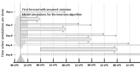
In case of a real volcanic eruption, several simulations are used and started as shown in Fig. 1. The purpose of the ev-eryday initial forecast with a default volcanic source is to provide a conservative first estimate of the dispersion. How-ever, because of the high uncertainty in source intensity and vertical profile as well as ash size distribution, the resulting concentrations are very uncertain. Thus, as soon as possi-ble, source receptor model simulations, with a unit emission (1 kg s−1)released every third hour over multiple emission heights, are started that are used as input data for a source inversion calculation (Stohl et al., 2011), shown in Fig. 1 as thick arrows. The goal of applying the inversion algorithm is to create a source term that causes the model simulation to be more similar to observations. A very early timing of these model simulations is not as crucial since the inversion algo-rithm is dependent on good satellite observations to constrain the solution, meaning that enough satellite observations at some distance from the volcano are required. The source re-ceptor simulations run for a 24 h forecast do not include fur-ther uncertainties longer in the forecasts, and are restarted the next day for another 24 h cycle. Model simulations with the inversion-derived emissions estimate (dashed lines) are expected to be ready before a new forecast meteorology in-put dataset is available, since the inversion calculation is not computationally demanding. More details on using the in-version method in a forecast setting are given in Steensen et al. (2017). The lengths of the source receptor model simula-tions are set here as an example of 3 days as the inversion study found that additional satellite observations are seen to have little effect on the emission term after 48 h. The ash may however stay in the domain for a longer time, so the model simulations with the optimized emission term have to be started from an earlier time.
3 Meteorological predictability of volcanic plumes: example SO2from Barðarbunga
Figure 1.Sequence of model simulations started at the Norwegian Meteorological Institute in the case of a volcanic eruption. The single black arrows indicate 48 h forecast simulations. The thick striped arrows represent the multiple model simulations started for the inversion algorithm to retrieve an improved emissions estimate using satellite data. Dashed lines represent spin-up model simula-tions with emissions estimates found by the inversion algorithm. These model simulations are continued as forecasts (single black arrows). The chronological order of simulations starts from the top, so new forecast results are available every 12 h. The inversion sim-ulations are restarted every 24 h.
compare model simulations for the Barðarbunga eruption to satellite and ground observations of SO2 and SOx wet de-position. A simplified emissions term is used where SO2is
released at a constant rate, uniformly distributed over three emissions heights, to see which height produces a simula-tion that matches better with observasimula-tions. With some dis-crepancies caused by the description of the planetary bound-ary layer also found in Schmidt et al. (2015) with the La-grangian NAME model and in Boichu et al. (2016) with the Eulerian CHIMERE model, the EMEP MSC-W model matches well the observed surface SO2timing and
concen-tration levels. Compared to SO2 column satellite
observa-tions from the Ozone Monitoring Instrument (OMI), similar mass loadings and dispersion patterns are found. However, it remains a question how much the uncertainty in the meteo-rological fields determines the quality of the volcanic plume predictability.
In meteorology, ensemble forecasts consist of several al-most identical simulations to quantify the uncertainty of a forecast. Large spread between the ensemble members caused by a large difference between possible future sce-narios indicates a high uncertainty in the forecast. Combin-ing the eEMEP model with ensemble forecasts would create an opportunity for quantifying the uncertainty in the eEMEP ash/SO2forecasting related to the uncertainty in the
meteo-rology. However, running the eEMEP model on several (tens of) ensemble forecast members (at a relatively high resolu-tion) is computationally a very expensive task. At the same time, the volcanic emission forecasting system is required to deliver results very quickly and several times a day. One might think at first that this leaves us with the choice be-tween a low resolution ensemble forecast and a high
resolu-tion deterministic forecast for the operaresolu-tional volcanic emis-sion forecasting system.
Here we investigate how the different resolutions of the en-semble forecasts affect the spread of the volcanic plume for SO2for 3 days at the beginning of the Barðarbunga eruption,
including the probability of the resulting SO2concentrations
in the different members being over different thresholds. Al-though this part focuses on volcanic emissions of SO2,
sim-ilar results may be expected for spread of the fine-grained long-range transported volcanic ash.
3.1 Model set-up
The eEMEP model is run on meteorological ensemble fore-cast data from the Grand Limited Area Ensemble Prediction Systems (GLAMEPS) for the Barðarbunga eruption case. The starting dates, 3 to 5 September 2014, from which the respective 48 h forecasts are launched, correspond to the first part of the Barðarbunga volcanic eruption.
Significant amounts of SO2 were ejected into the
at-mosphere during the Barðarbunga eruption, but little ash. Schmidt et al. (2015) studied the emissions term during September by comparing model simulations to satellite data, and found that a SO2 emissions estimate with a 120 kt d−1
flux uniformly over an eruption column between 1500 and 3000 m matched best for the first days of September. This emissions term is also supported by Thordarson and Hart-ley (2015) and used here. In an emergency case an a priori source term would be used first when little information about the volcanic source term is known. Using the same best guess source term here in all our ensemble model simulations of-fers the opportunity to study the results based on only the different weather situations, meteorology uncertainties, and resolution.
GLAMEPS meteorological data
GLAMEPS aims to account for all the major sources of weather forecast inaccuracy by including both the differences due to model parameter uncertainty and initial state perturba-tions (Iversen et al., 2011). GLAMEPS ensemble forecast is produced at ECMWF, and in 2014 the ensemble consisted of 50 members from both the HIRLAM (High Resolution Limited Area Model) and ALADIN (Aire Limitée Adapta-tion Dynamique Développement InternaAdapta-tional) models. To include uncertainty in the forecast, members are perturbed both in the initial field and on the model domain border. The perturbations are from the EuroTEPS (European Tar-geted Ensemble Prediction system), a version of the global ECMWF EPS, with higher resolution on a smaller European domain (Frogner and Iversen, 2011).
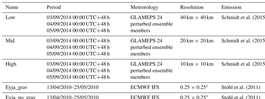
parameterisa-Table 1.List and names of model simulations used in this paper.
Name Period Meteorology Resolution Emission
Low 03/09/2014 00:00 UTC+48 h
04/09/2014 00:00 UTC+48 h 05/09/2014 00:00 UTC+48 h
GLAMEPS 24 perturbed ensemble members
40 km×40 km Schmidt et al. (2015)
Mid 03/09/2014 00:00 UTC+48 h
04/09/2014 00:00 UTC+48 h 05/09/2014 00:00 UTC+48 h
GLAMEPS 24 perturbed ensemble members
20 km×20 km Schmidt et al. (2015)
High 03/09/2014 00:00 UTC+48 h
04/09/2014 00:00 UTC+48 h 05/09/2014 00:00 UTC+48 h
GLAMEPS 24 perturbed ensemble members
10 km×10 km Schmidt et al. (2015)
Eyja_grav 13/04/2010–25/05/2010 ECMWF IFS 0.25×0.25◦ Stohl et al. (2011)
Eyja_no_grav 13/04/2010–25/05/2010 ECMWF IFS 0.25×0.25◦ Stohl et al. (2011)
tions. HirEPS_S members use the STRACO scheme (Sass et al., 1999; Undén et al., 2002) for stratiform, convective cloud and precipitation; HirEPS_K members use the Kain– Fritsch schemes for deep cumulus (Kain and Frisch, 1990; Kain, 2004; Calvo, 2007) and Rasch and Kristjansson (1998) for stratiform clouds and precipitation (Ivarsson, 2007). To also include the uncertainty in the forecast caused by the start time of the forecast, members are divided into two groups with two different forecast start times. Six members of the HirEPS_S and six of the HirEPS_K start the forecast at 00:00 and 12:00 UTC, and the remaining 12 ensemble members start the forecast at 06:00 and 18:00 UTC. All of the mem-bers are perturbed by using EuroTEPS. Each member has a forecast time of 72 h. The original resolution is 10×10 km; such a fine resolution is computationally very demanding.
The GLAMEPS data have been downloaded from ECMWF for the period from 3 to 5 September 2014, cor-responding to the first phase of the Barðarbunga volcanic eruption. Each member is used as input data for the eEMEP model to run 48 h forecasts starting from 00:00 UTC from each of the 3 days by using the 18 and 00:00 UTC meteoro-logical forecasts. That means that for half of the members, the forecast is 6 h old (the forecasted started at 18:00 UTC). The relatively short forecast of 48 h is chosen due to the large uncertainties related to the emission term when running a forecast of volcanic emission (VAAC London only issues a maximum 24 h forecast). Furthermore, running the full 72 h forecast is not feasible due to the different start times of the forecasts (18:00 and 00:00 UTC). In contrast to what is pos-sibly done for a real case, all the forecasts are started from a model state with no volcanic SO2in the atmosphere, and
are not restarted from the previous forecast simulation. This is done to investigate only the difference in spread due to the different weather situations over the 3 days studied, and does not take into account possible differences in the initial SO2
field.
Three different horizontal resolutions are generated as in-put: the original high resolution of 10×10 km, a medium resolution of 20×20 km, and a low resolution of 40×40 km, referenced hereafter as high_res, mid_res, and low_res. High resolution NWP is desired, as more processes in the atmo-sphere can be resolved. A simple reduction in resolution of the meteorological input data is obtained here by letting ev-ery other or evev-ery fourth original grid value become the grid value representing the coarser grid resolution respectively. Alternatively, one could have aggregated 10×10 km grid cells into 20×20 and 40×40 km grid cells. This would lead to a smoother field, but the largest values/variations would have been lost. The GLAMEPS domain covers an area from 16 to 81◦north and 67◦west to 83◦east, which means that Europe and the North Atlantic are well covered, including some parts of the Sahara and Newfoundland. There are 40 vertical levels for all three horizontal resolutions. Table 1 lists all simulations in this paper.
3.2 Results
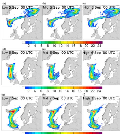
The spread in the ensemble forecast of SO2 is presented
here by calculating the possibility of an ensemble member being over certain threshold values. Figures 2 and 3 show the frequency of ensemble members over a low vertical col-umn density (VCD) of 5 DU (Dobson units) threshold and a high VCD threshold of 50 DU after 48 h forecast respec-tively. High and low thresholds are chosen as increased dilu-tion will lead to a larger area with lower column loads and a smaller area with higher column loads. For the first forecast starting on 3 September at 00:00 UTC, the SO2emitted from
Figure 2.Map of the number of ensemble members that locally ex-ceeds a 5 DU SO2limit. Counted after 48 h in the low, mid, and high
resolution ensembles, in the left, middle, and right columns respec-tively for start time 00:00 UTC on 3 September(a, b, c), 00:00 UTC on 4 September(d, e, f), and 00:00 UTC on 5 September(g, h, i).
Compared to the two higher resolution forecasts, the low_res forecasts have a large area where 20 or more mem-bers agree and have column loads over the 5 DU threshold after 48 h of dispersion. The mid_res and high_res simula-tions show however a larger spread between the members with a bigger area with only one or a few members above the low threshold. This larger spread among the higher res-olution forecast is also shown in Fig. 3. The high_res fore-cast have members that exceed the 50 DU threshold far away from the source, as seen over the coast of northern Russia in the first forecast (3 September 00:00 UTC+48 h) and also further down in the high pressure system appearing during the two later forecasts. Due to increased numerical diffusion in the low_res forecasts, the area where the members are over the higher threshold is much smaller and mostly confined to an area close to the source.
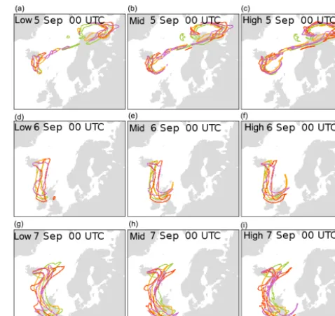
The difference in the spread is also seen to be weather dependent, especially when using a low threshold. Figure 4 shows the 5 DU contour line for the forecasts corresponding to Fig. 2, for four of the ensemble members. Each of the four members represents one of the perturbed members from the two different model parameterisations and starting times. For the first forecast started there are large differences between the members for areas where they have VCDs above 5 DU. In the second forecast started, the differences between the
Figure 3.The same as Fig. 2, counting ensemble members locally exceeding a 50 DU limit.
members are smaller, while the last forecast from 5 Septem-ber at 00:00 UTC shows that, although the memSeptem-bers all have plumes with VCDs over 5 DU going south from Iceland, they have quite different positions, indicating a different position of the low pressure system.
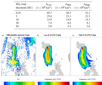
To further investigate the differences in the three resolu-tions, Table 2 shows the area summed up at time step+48 h for all the three forecasts where simulated SO2column loads
exceed the given threshold values. There is a 34 % larger area with column burdens above 0.25 DU in the low reso-lution forecasts compared to the high resoreso-lution forecasts, due to the increased diffusion. At 10 DU, the difference in area between the three resolutions is minimal, while for the thresholds above 10 DU the high resolution forecast exhibits a larger area.
a thin filament. Even though the total amount of area, where ensemble members show SO2column loads above the 10 DU
threshold, is found to be equal for the three resolutions, the high_res ensemble forecasts have members exhibiting fur-ther soufur-thern loads over the threshold. An area with high SO2column loads in the south-west is not captured by either
of the forecasts. Previous studies of this eruption (Schmidt et al., 2015; Steensen et al., 2016) show that this area is af-fected by older emissions compared to what is included in our model simulations that start at 00:00 UTC on 4 Septem-ber, and is thus not apparent in the model simulations pre-sented here.
The higher resolution ensemble members show higher concentrations further away from the volcanic eruption site in narrower SO2 clouds that resemble the observed SO2
clouds more. However, the location of the plumes varies more between the high resolution ensemble members, e.g. a larger spread between the ensemble members indicates a higher uncertainty. Although a lower uncertainty in a forecast is appreciated as it indicates that the weather situation is sta-ble, less spread in low resolution also indicates that informa-tion in the meteorology is lost when reducing the resoluinforma-tion. This suggests that running ensemble forecasts with low reso-lution for transport of volcanic emissions is less meaningful, as it would not show the actual uncertainty in the forecast.
Even though a high resolution is desirable, the computa-tional efficiency is important in an emergency forecast envi-ronment. For this study, the highest resolution runs use over 13 times more computational time than the lowest resolution runs, while the mid_res simulations use only 5 times more. To run a total ensemble forecast with high resolution for vol-canic eruptions may therefore not be feasible. From a prag-matic point of view, ensemble forecasts for volcanic emis-sions are most valuable in situations where the weather fore-cast is uncertain. Thus an alternative would be to launch en-semble forecasts only in unstable weather situations (as pre-dicted by the ensemble weather prediction models). As in this study, to exclusively look at the spread due to the uncertainty in the weather forecast, the same source term should be used in all the members. Therefore the model simulations used as input for the inversion calculations will only be driven by the deterministic meteorology. This study indicates that less information is lost between high_res and mid_res than go-ing from the mid_res to low_res resolutions, suggestgo-ing that resolutions around 20×20 km could be a reasonable choice for ensemble (and deterministic) forecasts when needed. Ide-ally, more studies should be done that include other weather situations as well as different types of eruptions, to draw con-clusions on the best grid resolution.
Figure 4.The 5 DU contour lines for four exemplary members af-ter 48 h of forecast in the low, mid, and high resolution ensembles, in the left, middle, and right columns respectively, for start time 00:00 UTC on 3 September(a, b, c), 00:00 UTC on 4 September (d, e, f), and 00:00 UTC on 5 September(g, h, i).
4 Ash model testing and validation
4.1 Model set-up
The eEMEP model with improved ash modelling capabili-ties as described above is tested here for the Eyjafjallajökull eruption in 2010. For this purpose the model is run with the emission term from Stohl et al. (2011), an emission term con-strained by satellite observations through an inversion rou-tine. The ash is distributed over nine size bins with charac-teristic sizes of 4, 6, 8, 10, 12, 14, 16, 18, and 25 µm (with a lower limit of 3 µm and an upper limit of 28 µm); the ash in the source term is distributed among the bins as follows: 16, 18, 15, 13, 10, 8, 6, 7, and 7 %. The density is set by default to 2500 kg m−3. Our eEMEP model uses here meteorological data from ECMWF, namely the IFS (Integrated Forecasting System) model with a 0.25×0.25◦latitude longitude resolu-tion, selecting 42 of the lower levels from the original IFS 60 vertical levels, and setting the eEMEP model top to around 30 km. The simulations are performed for the volcanic ash eruption episode from 13 April to 25 May 2010.
4.2 Comparison with other ash models
Table 2. Total area A where SO2loads are above a given threshold, found on average in members of the low, mid, and high resolution ensembles (see Table 1). Areas are accumulated at the end of a 48 h forecast, corresponding to Figs. 1 and 2.
SO2load ALow AMid AHigh
threshold (DU) (1×10⁶km2) (1×10⁶km2) (1×10⁶km2)
0.25 69.7 58.3 52.1
5 25.0 23.1 21.3
10 14.9 14.8 14.3
20 7.4 8.0 8.1
50 2.0 2.4 2.6
Figure 5.OMI retrieval of SO2(left) for the satellite overpasses between 08:00 and 16:00 UTC on 5 September. Frequency of ensemble
members over 10 DU for the low (middle) and high (right) resolution runs. Frequencies are computed every hour and averaged over the same time period, using the forecast runs started on 4 September 00:00 UTC.
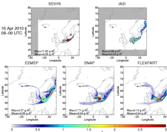
model SNAP (Saltbones et al., 1994), and found very sim-ilar ash plumes in all three models (Norwegian ash project, 2014). Figure 6 shows results where all three model results are compared to satellite ash retrievals from SEVIRI (Spin-ning Enhanced Visible and Infrared Imager) and IASI (In-frared Atmospheric Sounding Interferometer) available from http://vast.nilu.no/. The FLEXPART model is used in sev-eral studies and validated towards observations for sevsev-eral volcanic eruptions with ash emission (Stohl et al., 2011; Kristiansen et al., 2012; Moxnes et al., 2014). All models use the same wind fields from ECMWF, and the conclusion for this eruption case was that neither the Eulerian nor the Lagrangian models showed particularly better performance. The structure and intensity of the plumes was rather similar, reproducing the observations fairly well when it comes to the ash fields.
4.3 Validation with lidar observations
Apart from the horizontal dispersion, the vertical placement of the transported ash may have important consequences for impact assessments, both for air quality and air traffic per-turbations. Meteorological processes such as subsidence and
frontal lifting may alter the initial vertical distribution of ash. In addition, ash removal and settling may alter the vertical distribution. Although several observational sets are avail-able for the Eyjafjallajökull eruption, to test here the treat-ment of gravitational settling for ash particles in the eEMEP model, model results with and without gravitational settling of ash included are compared to lidar observations of the ash layer.
Figure 6.Mean ash column burdens from 08:00 to 09:00 UTC on 16 April for SEVIRI and IASI satellite ash retrievals, and eEMEP, SNAP, and FLEXPART model simulations.
as well as the centre of mass, the altitude where most of the aerosol load is located. Identified ash layers where other aerosol sources are also found from e.g. continental aerosol are classified as mixed layers. These mixed layers are also given with the maximum and minimum observed height and centre of mass. Observed planetary boundary layer (PBL) height is also included in the database. The six lidar sta-tions used here are situated in central Europe (see Fig. 7), covering coastal stations and inland and mountain regions. Weather conditions at the lidar stations, and sometimes tech-nical issues, made it difficult to continuously produce obser-vations. For example, frequent low clouds over Cabauw pre-vented most lidar retrievals there. Observations at Neuchatel are also limited to the first episode in April. Altogether, the ash layer was observed over a long period over central Eu-rope during the Eyjfjallajökull eruption and, as the ash has been transported over a long distance, the effect of gravita-tional settling may be visible for the fine ash particles, mak-ing this dataset the best available at the time for our purpose. Webley et al. (2012) found by studying model results from WRF-Chem that ash particles larger than 62.5 µm were not transported further than 120 km from the volcano, indicating that ash particles larger than what are included in this study have already fallen out by the time the air mass reaches the lidar sites and will not affect the observed ash layer.
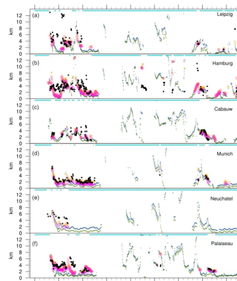
Figure 8 shows the model concentrations for the simu-lation with gravitational settling over the entire Eyjafjalla-jökull period along with observed height of the ash layer and
Figure 7.Map of EARLINET lidar measurement sites used in the study.
Figure 8. Height–time profiles of ash concentrations from the eEMEP model, including gravitational settling, at the six EAR-LINET lidar stations (see Fig. 6) in the April–May 2010 episode (contour graph in the background). Lidar-detected upper and lower heights of the ash layer are presented as grey dots. The lidar-retrieved centre of mass for ash is plotted as black dots. For mixed layers where ash is identified with continental aerosol, the height of the layer is presented as light pink dots, and centres of mass are red dots. The height of the planetary boundary layer is shown in vi-olet. Due to weather conditions and technical difficulties, the lidar measurements are not a continuous series.
Ash was first detected at the Hamburg station during the morning of 16 April, 48 h after the start of the eruption. Ash was also observed early at the other stations, and while the timing of the observations matches well at Hamburg and Leipzig, at Neuchatel ash is observed before the model has transported ash to this station. At Cabauw, the first part of the ash plume is not covered by the lidar because no measure-ments are available, while the second part shows similar sim-ulated and observed levels of maximum concentrations. Even though a lidar does not measure concentrations, it is possible to retrieve these using mass-to-extinction coefficients. Ans-mann et al. (2011) and Wiegner et al. (2012) estimated maxi-mum ash concentrations of around 1100 µg m−3with around 40 % uncertainty over Hamburg and Munich (lidar actually
Figure 9.Modelled and observed centres of mass for ash at the li-dar stations. Green and blue dots represent the centre of ash mass, computed from the entire model column, for simulations with and without gravitational settling, shown where ash concentrations were larger than 0.1 µg m−3. Magenta and orange represent the model centre of ash, calculated above the observed planetary boundary layer (PBL) with and without gravitational settling respectively. Black dots are the corresponding lidar retrieved centre of mass for ash above the PBL (same as Fig. 7). The light blue line above indi-cates where observations are missing.
26 April; model and observed ash layers are mostly at sim-ilar heights for this later April period. There are some dis-crepancies: for Cabauw the observations vary in height over short time periods, indicating uncertainties for these mea-surements, and in Munich, the maximum heights of the ob-served ash layer are at higher altitudes than the model maxi-mum ash height, while the observed centres of mass are close to the observed lowest layer of ash, indicating that most of the ash mass indeed is lower in the atmosphere and more comparable to model heights. In Leipzig a few observations of centre of mass on 16 and 18 April are much higher (at 12 km) than the model centre of mass heights and the corre-sponding heights at the other stations at this time, implying these high altitude measurements may not represent ash.
From 2 May the model results show small ash concentra-tions at the lidar staconcentra-tions, due to small ash emissions after 29 April. On 5–6 May ash is observed lower down in the at-mosphere compared to simulated ash at Hamburg; however, a layer where ash is mixed with other aerosols is detected at higher altitudes more similar to where the model has ash. More ash was then emitted on 5 May (Stohl et al., 2011), but southerly winds transported the ash over Spain and the At-lantic Ocean. Not until the night of 16/17 May are weather conditions favourable again for transport of ash to central Eu-rope. No measurements are available for this time at Neucha-tel. The other stations have observations of the ash layer at similar altitudes to the model. Ash concentrations estimated over Cabauw on 17 May are around 500 µg m−3, around half of what is found in April (Ansmann et al., 2011).
To show more broadly the impact of the gravitational set-tling processes on the vertical profile of ash, Fig. 8 shows all calculated centres of mass for ash in the model simulation with and without gravitational settling. The rather small dis-placement between the two model simulations implies that not gravitation, but rather weather and emission height, are the main drivers of the ash layer height. This is especially vis-ible in the simultaneous rapid decrease in the centre of mass height for the first plume (17–18 April) in both simulations. On some occasions there are larger differences between the two model simulations, specifically in the beginning of May during a period with smaller concentrations. Unstable north-westerly winds at this time can cause the small differences in height distribution of ash to grow over time due to different wind directions in the column.
In order to compare to the observed values more properly, a centre of mass above the observed PBL is calculated for the two model simulations (only for the cases when an observed height is available); see Fig. 8. Model centres of mass are generally lower than observed altitudes for both model simu-lations, indicating that the model simulations have too much descent of the ash layer e.g. around 18 April, independent of inclusion or not of gravitational settling. Figure 10 show scatterplots where the observed ash centre of mass height (not including the mixed layers) is plotted against the model with and without gravitational settling at the stations. As
dis-cussed above, some measured and modelled values are unre-alistically high; therefore, only values below 8 km are taken into account for correlation calculations. The scatterplot con-firms that observed heights are generally higher than model calculations. At Palaiseau and Hamburg, model height de-scends faster than observed on 20 April, causing the low correlation at these stations. Neuchatel generally exhibits a higher observed centre of mass, explaining possibly a slightly higher correlation for the model simulation with no gravi-tational settling. Except for Neuchatel and Hamburg, how-ever, the model simulation with gravitational settling exhibits a slightly higher correlation with lidar-retrieved height data compared to the model simulation without gravitation.
5 Summary and conclusions
A new model version of the standard EMEP MSC-W model has been developed, aimed at modelling dispersion of vol-canic emission, called the eEMEP model. Changes with re-spect to the standard model are a simplified gas chemistry; a modification of the aerosol part to handle ash particles in dif-ferent size classes; the description of gravitational settling of ash particles; a volcanic source module which has a default source term and can be altered to include improved source estimates; an increase in vertical levels to increase the model top and vertical resolution; the possibility to run as an en-semble model based on enen-semble meteorological forecasts; a formal procedure for an operational use of the model in an emergency case; and an inversion algorithm coupled to the model, using satellite data to retrieve an improved source es-timate (Steensen et al., 2017). With this model version we document here selected important aspects of the volcanic gas and ash dispersion simulation.
We have first studied the impact of ensemble meteorolog-ical input fields of different resolutions on the dispersion of volcanic emissions from Iceland. Compared to Lagrangian VATDMs, Eulerian models such as the eEMEP model have inherent numerical diffusion dependent on the grid size. eEMEP model simulations thus have to have a sufficiently high resolution, especially when peak concentrations shall be predicted, for example for the purpose of establishing flight restriction zones. High resolution simulations are however computationally demanding, while obtaining results quickly is critical in situations with volcanic eruptions. How to best use CPU resources for transport of volcanic emission is stud-ied here by looking at the change in spread between ensemble model simulations at three different resolutions. The eEMEP model is run for a 48 h forecast from three start dates for the Barðarbunga eruption period with meteorological fields from 24 HIRLAM ensemble members originally produced for the GLAMEPS forecast. The original 10×10 km resolution is degraded to lower resolutions of 20×20 and 40×40 km.
reso-Figure 10.Scatterplots for observed versus simulated centres of ash mass with (magenta) and without (orange) gravitational settling. Data correspond to Fig. 8 using model and observed values under 8 km but above the PBL. Correlation between observed and model values is given in the upper left corner.
lution simulations than in the high resolution ones. For the higher resolution forecast simulations, the members show more spread between them and there are members with higher concentrations further away from the source. There-fore there is also a greater possibility of a member exceed-ing a high threshold concentration. For all three simulations, the spread between members is seen to be weather depen-dent and a measure for how uncertain the forecast is. The increased agreement between low resolution ensembles due to increased numerical diffusion limits the importance of the ensemble forecast. Ensemble forecasts have to be done with sufficiently high resolution to show the real uncertainty of the weather situation. Compared to satellite observations, the high resolution model simulations also match better the transport of a narrow volcanic SO2cloud. High resolution
en-semble forecast may nevertheless not be possible due to the computational cost. The study shows that there is a bigger change in transport when going from 40×40 to 20×20 km resolution compared to 20×20 to 10×10 km, indicating that the increased cost of running a high resolution simulation at 10×10 km may not give the same increase in the quality of the result. The study also shows that low resolution simula-tions are sufficient for quick results to predict the most likely
transport of volcanic emission, while high resolution model simulations are needed to assess the possible occurrence of high peak concentrations.
the Hamburg and Leipzig lidar stations. A second descent in the ash layer at the stations is seen on 20 April, and this subsidence occurs later in the observational data at Hamburg and Palaiseau compared to the model data. The model has a centre of ash mass height on average below the observed one, independent of gravitational settling. Calculated lation between observed centres of mass height and corre-sponding model heights are higher in the model simulation, with gravitational settling for four of the six stations stud-ied here, suggesting improved quality of the model when in-cluding the gravitation process. The addition of gravitational settling is found to have a relatively small influence on the vertical placement of the ash layer and thus is responsible only for a small improvement in model results. The model simulations presented here only include ash sizes of up to 25 µm in diameter, and including larger ash particles in the calculations can show a larger effect.
Even with the included gravitational settling in the EMEP model, the assumed density, shape, and size distribution of the ash particles bring along large uncertainties during a fore-cast situation. Ash properties show large differences in be-tween volcanic eruptions (Vogel et al., 2016). The Eyjaf-jallajökull model results presented here are initiated with a time and height resolved emissions estimate calculated by inversion with FLEXPART model results, constrained with satellite observations (Stohl et al., 2011), to be used with the eEMEP model for a new volcanic eruption in an operational set-up. Uncertainties in satellite retrievals due to meteorolog-ical clouds that obscure ash clouds and a 0.2 g m−2ash cloud detection limit (Prata and Prata, 2012) need to be explored further. Low concentrations in satellite and model data are in particular uncertain, as shown during the intermediate pe-riod (end of April and beginning of May) when only small emissions were released and then observed at the lidar sta-tions as almost insignificant ash clouds. Another large factor of uncertainty is the variability in ash particle sizes, which changed between the first eruption period in April and the second in May (Dellino et al., 2012). Both model and satellite retrievals, used as input to the inversion, operate today with assumed equal ash characteristics during the whole eruption period. Other processes, such as fine ash aggregation that in-creases the gravitational settling speed and reduces the atmo-spheric residence time (Brown et al., 2011), were also ob-served during the Eyjafjallajökull eruption (Taddeucci et al., 2011), but are not included in the model at this time.
Although a correct model description of bulk volcanic emissions is useful, other factors such as model resolution, details of the source term, and the model set-up are seen as important for safety assessments. The developed model is ca-pable of guiding near real time emergency assessments of the spread of high volcanic gas and aerosol concentrations.
Code availability. The model code to the standard EMEP MSC-W model is available on github: https://github.com/metno/emep-ctm. The eEMEP model with reduced chemistry and gravitational set-tling for ash is available here: https://github.com/metno/emep-ctm/ releases/tag/rv4_10_eEMEP_ASH.
Competing interests. The authors declare that they have no conflict of interest.
Acknowledgements. The authors would like to thank Fred Prata and Lieven Clarisse for SEVIRI and IASI satellite data for the model comparison and Nina I. Kristiansen for numerous inspiring discussions and technical help. We also thank Inger-Lise Frogner for the valuable help with obtaining GLAMEPS data. We thankfully acknowledge the EARLINET lidar data providers for assembling a very useful lidar dataset. This work has also received funding under the ACTRIS project from the European Union’s Horizon 2020 research and innovation programme under grant agreement no. 654109. The work done for this paper is funded by the Norwegian ash project financed by the Norwegian Ministry of Transport and Communications and AVINOR. Model and support are also appreciated through the Cooperative Programme for Monitoring and Evaluation of the Long-range Transmission of Air Pollutants in Europe (no. ECE/ENV/2001/003). This work has also received support from the Research Council of Norway (Programme for Supercomputing) through CPU time granted at the supercomputers at NTNU in Trondheim.
Edited by: A. Colette
Reviewed by: two anonymous referees
References
Ansmann, A., Tesche, M., Seifert, P., Gross, S., Freudenthaler, V., Apituley, A., Wilson, K. M., Serikov, I., Linne, H., Heinold, B., Hiebsch, A., Schnell, F., Schmidt, J., Mattis, I., Wandinger, U., and Wiegner, M.: Ash and fine-mode particle mass profiles from EARLINET-AERONET observations over central Europe after the eruptions of the Eyjafjallajökull volcano in 2010, J. Geophys. Res.-Atmos., 116, D00U02, doi:10.1029/2010JD015567, 2011. Boichu, M., Chiapello, I., Brogniez, C., Péré, J.-C., Thieuleux,
F., Torres, B., Blarel, L., Mortier, A., Podvin, T., Goloub, P., Söhne, N., Clarisse, L., Bauduin, S., Hendrick, F., Theys, N., Van Roozendael, M., and Tanré, D.: Current challenges in modelling far-range air pollution induced by the 2014–2015 Bárðarbunga fissure eruption (Iceland), Atmos. Chem. Phys., 16, 10831– 10845, doi:10.5194/acp-16-10831-2016, 2016.
Bott, A.: A positive definite advection scheme obtained by nonlin-ear re-normalization of the advection fluxes, Mon. Weather Rev., 117, 1006–1015, 1989a.
Bott, A.: Reply, Mon. Weather Rev., 117, 2633–2636, 1989b. Brown, R. J., Bonadonna, C., and Durant, A. J.: A review of
vol-canic ash aggregation, Phys. Chem. Earth, 45–46, 65–78, 2011. Calvo, J.: Kain-Fritsch convection in HIRLAM, Present status and
Casadevall, T. J.: Volcanic ash and aviation safety: Prodeedings of the First International Symposium on Volcanic Ash and Aviation Safety, U.S. Geol. Surv. Bull., 2047, 450 pp., 1994.
Dellino, P., Gudmundsson, M. T., Larsen, G., Mele, D., Steven-son, J. A., ThordarSteven-son, T., and Zimanowski, B.: Ash from the Eyjafjallajökull eruption (Iceland): Fragmentation processes and aerodynamic behavior, J. Geophys. Res., 117, B00C04, doi:10.1029/2011JB008726, 2012.
Draxler, R. R. and Hess, G.: Description of the HYSPLIT_4 mod-eling system NOAA Tech. Memo. ERL ARL-224, NOAA Air Resources Laboratory, Silver Spring, MD 24 pp., 1997. Emeis, S., Forkel, R., Junkermann, W., Schäfer, K., Flentje, H.,
Gilge, S., Fricke, W., Wiegner, M., Freudenthaler, V., Groß, S., Ries, L., Meinhardt, F., Birmili, W., Münkel, C., Obleitner, F., and Suppan, P.: Measurement and simulation of the 16/17 April 2010 Eyjafjallajökull volcanic ash layer dispersion in the northern Alpine region, Atmos. Chem. Phys., 11, 2689–2701, doi:10.5194/acp-11-2689-2011, 2011.
EMEP Status Report 1/2016: Transboundary particulate matter, photo-axidants, acidifying and eutrophying components, EMEP MSC-W & CCC & CEIP, Norwegian Meteorlogical Institute (EMEP MSC-W), Oslo, Norway, 2016.
Folch, A., Costa, A., and Macedonio, G.: FALL3D: A computa-tional model for transport and deposition of volcanic ash, Com-put. Geosci, 35 1334–1342, doi:10.1016/j.cageo.2008.08.008, 2009.
Folch, A., Costa, A., and Basart, S.: Validation of the FALL3D ash dispersion model using observations of the 2010 Eyjafjallajökull volcanic ash clouds, Atmos. Environ., 48, 165–183, 2012. Frogner, I.-L. and Iversen, T.: EuroTEPS – a targeted version of
ECMWF EPS for the European area, Tellus A, 63.3, 415–428, 2011.
Ivarsson, K. I.: The Rasch Kristjansson large scale condensation. Present status and prospects, HIRLAM Newslett, 52, 50–56, 2007.
Iversen, T., Deckmyn, A., Santos, C., Sattler, K., Bremnes, J. B., Feddersen, H., and Frogner, I.-L.: Evaluation of ‘GLAMEPS’ – a proposed multimodel EPS for short range forecasting, Tellus A, 63, 513–530, doi:10.1111/j.1600-0870.2010.00507.x, 2011. Jacobson, M. Z.: Fundamentals of atmospheric modeling,
Cam-bridge University Press, 1991.
Jones, A., Thomson, D., Hort, M., and Devenish, B.: The UK Met Office’s next generation atmospheric dispersion model, NAME III, in: Air Pollution Modelling and its Application XVII, edited by: Borrego, C. and Norman, A.-L., 580–589, Springer, New York, 2007.
Josse, B., Simon, P., and Peuch, V.-H.: Radon global simulation-swith the multiscale chemistry and transport model MOCAGE, Tellus B, 56, 339–356, doi:10.1111/j.1600-0889.2004.00112.x, 2004.
Kain, J. S.: The Kain-Fritsch Convective Parameterization, Anup-date, J. Appl. Meteorol., 43, 170–181, 2004.
Kain, J. S. and Fritsch, J. M.: A one-dimensional entrain-ing/detraining plume model and its application in convective pa-rameterization, J. Atmos. Sci., 47, 2784–2802, 1990.
Kristiansen, N. I., Stohl, A., Prata, A. J., Bukowiecki, N., Dacre, H., Eckhardt, S., Henne, S., Hort, M. C., Johnson, B. T., Marenco, F., Neininger, B., Reitebuch, O., Seibert, P., Thomson, D. J., Web-ster, H. N., and Weinzierl, B.: Performance assessment of a
vol-canic ash transport model mini-ensemble used for inverse model-ing of the 2010 Eyjafjallajök ull eruption, J. Geophys. Res., 117, D00U11, doi:10.1029/2011JD016844, 2012.
Marécal, V., Peuch, V.-H., Andersson, C., Andersson, S., Arteta, J., Beekmann, M., Benedictow, A., Bergström, R., Bessagnet, B., Cansado, A., Chéroux, F., Colette, A., Coman, A., Curier, R. L., Denier van der Gon, H. A. C., Drouin, A., Elbern, H., Emili, E., Engelen, R. J., Eskes, H. J., Foret, G., Friese, E., Gauss, M., Giannaros, C., Guth, J., Joly, M., Jaumouillé, E., Josse, B., Kady-grov, N., Kaiser, J. W., Krajsek, K., Kuenen, J., Kumar, U., Li-ora, N., Lopez, E., Malherbe, L., Martinez, I., Melas, D., Meleux, F., Menut, L., Moinat, P., Morales, T., Parmentier, J., Piacentini, A., Plu, M., Poupkou, A., Queguiner, S., Robertson, L., Rouïl, L., Schaap, M., Segers, A., Sofiev, M., Tarasson, L., Thomas, M., Timmermans, R., Valdebenito, Á., van Velthoven, P., van Versendaal, R., Vira, J., and Ung, A.: A regional air quality fore-casting system over Europe: the MACC-II daily ensemble pro-duction, Geosci. Model Dev., 8, 2777–2813, doi:10.5194/gmd-8-2777-2015, 2015.
Mastin, L. G.: A user-friendly one-dimensional model for wet vol-canic plumes, Geochemistry, Geophysics, Geosystems 8.3, 2007. Mastin, L. G., Guffanti, M., Servranckx, R., Webley, P., Barsotti, S., Dean, K., Durant, A., Ewert, J. W., Neri, A., Rose, W. I., Schneider, D., Siebert, L., Stunderj, B., Swansonk, G., Tupperl, A. Volentikm, A., and Waythomash, G. F.: A multidisciplinary effort to assign realistic source parameters to models of volcanic ash-cloud transport and dispersion during eruptions. J. Volcanol. Geotherm. Res., 1, 10–21, 2009.
Moxnes, E. D., Kristiansen, N. I., Stohl, A., Clarisse, L., Durant, A., Weber, K., and Vogel, A.: Separation of ash and sulfur dioxide during the 2011Grímsvötn eruption, J. Geophys. Res.-Atmos., 119, 7477–7501, doi:10.1002/2013JD021129, 2014.
Norwegian ash project (Kristiansen, N. I., Steensen, B. M., Klein, H., Fagerli, H., and Bartnicki, J.): Norwegain ash project report 2.3.1, internal report, available at request, 2014.
Palmer, T. N.: Predicting uncertainty in forecasts of weather and climate, Rep. Prog. Phys., 63, 71–116, 2000.
Palmer, T. N., Molteni, F., Mureau, R., Buizza, R., Chapelet, P., and Tribbia, J.: Ensemble prediction, Proceedings of the ECMWF Seminar on Validation of models over Europe (Vol. 1), 1993. Pappalardo, G., Mona, L., D’Amico, G., Wandinger, U., Adam, M.,
Amodeo, A., Ansmann, A., Apituley, A., Alados Arboledas, L., Balis, D., Boselli, A., Bravo-Aranda, J. A., Chaikovsky, A., Com-eron, A., Cuesta, J., De Tomasi, F., Freudenthaler, V., Gausa, M., Giannakaki, E., Giehl, H., Giunta, A., Grigorov, I., Groß, S., Haeffelin, M., Hiebsch, A., Iarlori, M., Lange, D., Linné, H., Madonna, F., Mattis, I., Mamouri, R.-E., McAuliffe, M. A. P., Mitev, V., Molero, F., Navas-Guzman, F., Nicolae, D., Pa-payannis, A., Perrone, M. R., Pietras, C., Pietruczuk, A., Pisani, G., Preißler, J., Pujadas, M., Rizi, V., Ruth, A. A., Schmidt, J., Schnell, F., Seifert, P., Serikov, I., Sicard, M., Simeonov, V., Spinelli, N., Stebel, K., Tesche, M., Trickl, T., Wang, X., Wag-ner, F., WiegWag-ner, M., and Wilson, K. M.: Four-dimensional dis-tribution of the 2010 Eyjafjallajökull volcanic cloud over Europe observed by EARLINET, Atmos. Chem. Phys., 13, 4429–4450, doi:10.5194/acp-13-4429-2013, 2013.
In-frared Imager measurements, J. Geophys. Res., 117, D00U23, doi:10.1029/2011JD016800, 2012.
Rasch, P. J. and Kristjánsson, J. E.: A comparison of the CCM3 model climate using diagnosed and predicted condensate param-eterizations, J. Climate, 11, 1587–1614, 1998.
Rose, W. I. and Durant, A. J.: Fine ash content of explosive erup-tions, J. Volcanol. Geotherm. Res., 186.1, 32–39, 2009. Saltbones, J., Foss, A., and Bartnicki, J.: SNAP: Severe Nuclear
Accient Program. Technical Description, Research Report No. 15, Norwegian Meteorological Office, Oslo, Norway, 1994. Sass, B. H., Nielsen, N. W., Jørgensen, J. U., and Amstrup, B.: The
Operational HIRLAM System at DMI, DMI Tech Rep. no 99–21, Danmarks Meteorologiske Institutt, Lyngby v. 100, Copenhagen, Denmark, 1999.
Schmidt, A., Leadbetter, S., Theys, N., Carboni, E., Witham, C. S., Stevenson, J. A., Birch, C. E., Thordarson, T., Turnock, S., Barsotti, S., Delaney, L., Feng, W., Grainger, R. G., Hort, M. C., Höskuldsson, Á., Ialongo, I., Ilyinskaya, E., Jóhannsson, T., Kenny, P., Mather, T. A., Richards, N. A. D., and Shepherd, J.: Satellite detection, long-range transport, and air quality impacts of volcanic sulfur dioxide from the 2014–2015 flood lava erup-tion at Bárðarbunga (Iceland), J. Geophys. Res.-Atmos., 120, 9739–9757, doi:10.1002/2015JD023638, 2015.
Schwaiger, H. F., Denlinger, R. P., and Mastin, L. G.: Ash3d: A finite-volume, conservative numerical model for ash trans-port and tephra deposition, J. Geophys. Res., 117, B04204, doi:10.1029/2011JB008968, 2012.
Searcy, C., Dean, K., and Stringer, W.: PUFF: A high-resolution volcanic ash tracking model, J. Volcanol. Geotherm. Res., 80, 1– 16, 1998.
Sears, T. M., Thomas, G. E., Carboni, E., Smith, A. J. A., and Grainger, R. G.: SO2 as a possible proxy for volcanic ash in
aviation hazard avoidance, J. Geophys. Res.-Atmos., 118, 5698– 5709, 2013.
Simpson, D., Benedictow, A., Berge, H., Bergström, R., Emberson, L. D., Fagerli, H., Flechard, C. R., Hayman, G. D., Gauss, M., Jonson, J. E., Jenkin, M. E., Nyíri, A., Richter, C., Semeena, V. S., Tsyro, S., Tuovinen, J.-P., Valdebenito, Á., and Wind, P.: The EMEP MSC-W chemical transport model – technical descrip-tion, Atmos. Chem. Phys., 12, 7825–7865, doi:10.5194/acp-12-7825-2012, 2012.
Steensen, B. M., Schulz, M., Theys, N., and Fagerli, H.: A model study of the pollution effects of the first 3 months of the Holuhraun volcanic fissure: comparison with observations and air pollution effects, Atmos. Chem. Phys., 16, 9745–9760, doi:10.5194/acp-16-9745-2016, 2016.
Steensen, B. M., Kylling, A., Kristiansen, N. I., and Schulz, M.: Uncertainty assessment and applicability of an inversion method for volcanic ash forecasting, Atmos. Chem. Phys. Discuss., doi:10.5194/acp-2016-1075, in review, 2017.
Stohl, A., Forster, C., Frank, A., Seibert, P., and Wotawa, G.: Technical note: The Lagrangian particle dispersion model FLEXPART version 6.2, Atmos. Chem. Phys., 5, 2461–2474, doi:10.5194/acp-5-2461-2005, 2005.
Stohl, A., Prata, A. J., Eckhardt, S., Clarisse, L., Durant, A., Henne, S., Kristiansen, N. I., Minikin, A., Schumann, U., Seibert, P., Stebel, K., Thomas, H. E., Thorsteinsson, T., Tørseth, K., and Weinzierl, B.: Determination of time- and height-resolved vol-canic ash emissions and their use for quantitative ash
disper-sion modeling: the 2010 Eyjafjallajökull eruption, Atmos. Chem. Phys., 11, 4333–4351, doi:10.5194/acp-11-4333-2011, 2011. Taddeucci, J., Scarlato, P., Montanaro, C., Cimarelli, C., Del
Bello, E., Freda, C., Andronico, D., Gudmundsson, M. T., and Dingwell, D. B.: Aggregation-dominated ash settling from the Eyjafjallajökull volcanic cloud illuminated by field and laboratory high-speed imaging, Geology, 39, 891–894, doi:10.1130/G32016.1, 2011.
Theys, N., De Smedt, I., van Gent, J., Danckaert, T.,Wang, T., Hen-drick, F., Stavrakou, T., Bauduin, S., Clarisse, L., Li, C., Krotkov, N., Yu, H., Brenot, H., and Van Roozendael, M.: Sulphur diox-ide vertical column DOAS retrievals from the Ozone Monitor-ing Instrument: Global observations and comparison to ground-based and satellite data, J. Geophys. Res.-Atmos., 120, 2470– 2491, doi:10.1002/2014JD022657, 2015.
Thomas, H. E. and Prata, A. J.: Sulphur dioxide as a volcanic ash proxy during the April–May 2010 eruption of Eyjafjalla-jökull Volcano, Iceland, Atmos. Chem. Phys., 11, 6871–6880, doi:10.5194/acp-11-6871-2011, 2011.
Thordarson, T. and Hartley, M.: Atmospheric sulphur loading by the ongoing Nornahraun eruption, North Iceland, EGU General Assembly Conference Abstracts, 17, 2015EGUGA, 1710708T, 2015.
Toth, Z. and Kalnay, E.: Ensemble forecasting at NMC: The gen-eration of perturbations, B. Am. Meteorol. Soc., 74, 2317–2330, 1993.
Vogel, A. Diplas, S., Durant, A. J., Azar, A. S., Rose, W. I., Sytchkova, A., Bonadonna, C., Krüger, K., and Stohl, A.: Ref-erence dataset of volcanic ash physicochemical and optical prop-erties, J. Geophys. Res., submitted, 2016.
Vogel, H., Förstner, J., Vogel, B., Hanisch, T., Mühr, B., Schättler, U., and Schad, T.: Time-lagged ensemble simulations of the dis-persion of the Eyjafjallajökull plume over Europe with COSMO-ART, Atmos. Chem. Phys., 14, 7837–7845, doi:10.5194/acp-14-7837-2014, 2014.
Webley, P. W., Steensen, T., Stuefer, M., Grell, G., Freitas, S., and Pavolonis, M.: Analyzing the Eyjafjallajökull 2010 erup-tion using satellite remote sensing, lidar and WRF-Chem dis-persion and tracking model, J. Geophys. Res., 117, D00U26, doi:10.1029/2011JD016817, 2012.
Wiegner, M., Gasteiger, J., Groß, S., Schnell, F., Freudenthaler, V., and Forkel, R.: Characterization of the Eyjafjallajökull ash-plume: Potential of lidar remote sensing, Phys. Chem. Earth, 45– 46, 79–86, doi:10.1016/j.pce.2011.01.006, 2012.
Wilson, L. and Huang, T. C.: The influence of shape on the atmo-spheric settling velocity of volcanic ash particles, Earth Planet. Sci. Lett., 44, 311–324, 1979.
Wilson, T. M., Stewart, C., Sword-Daniels, V., Leanard, G. S., John-ston, D. M., Cole, J. W., Wardman, J., Wilson, G., and Barnard, S. T.: Volcanic ash impacts on critical infrastructure, J. Phys. Chem. Earth, 45–46, 5–23, doi:10.1016/j.pce.2011.06.006, 2011. UK Civil Aviation Authority: A history of ash and aviation,
avail-able at: https://www.caa.co.uk/Safety-initiatives-and-resources/ Safety-projects/Volcanic-ash/A-history-of-ash-and-aviation/ (last access: 12 December 2016), 2016.