Forecasts covering one month using a cut-cell model

(1)

Geosci. Model Dev., 6, 875–882, 2013 www.geosci-model-dev.net/6/875/2013/ doi:10.5194/gmd-6-875-2013

EGU Journal Logos (RGB)

Advances in

Geosciences

Open Access

Natural Hazards

and Earth System

Sciences

Open Access

Annales

Geophysicae

Open Access

Nonlinear Processes

in Geophysics

Open Access

Atmospheric

Chemistry

and Physics

Open Access

Atmospheric

Chemistry

and Physics

Open Access Discussions

Atmospheric

Measurement

Techniques

Open Access

Atmospheric

Measurement

Techniques

Biogeosciences

Open Access Open Access

Biogeosciences

Discussions

Climate

of the Past

Climate

of the Past

Discussions

Earth System

Dynamics

Earth System

Dynamics

Discussions

Geoscientific

Instrumentation

Methods and

Data Systems

Open Access

_{Geoscientific}

Instrumentation

Methods and

Data Systems

Geoscientific

Model Development

Geoscientific

Model Development

Discussions

Hydrology and

Earth System

Sciences

Open Access

Hydrology and

Earth System

Sciences

Ocean Science

Discussions

Solid Earth

Discussions

The Cryosphere

Discussions

Natural Hazards

and Earth System

Sciences

Open Access

Discussions

Forecasts covering one month using a cut-cell model

J. Steppeler1, S.-H. Park2, and A. Dobler3

1_{Climate Service Center, Hamburg, Germany}

2_{National Center for Atmospheric Research, Boulder, Colorado, USA} 3_{Freie Universit¨at Berlin, Institute of Meteorology, Berlin, Germany}

Correspondence to: A. Dobler ([email protected])

Received: 21 December 2012 – Published in Geosci. Model Dev. Discuss.: 25 January 2013 Revised: 22 May 2013 – Accepted: 24 May 2013 – Published: 3 July 2013

Abstract. This paper investigates the impact and potential

use of the cut-cell vertical discretisation for forecasts cover-ing five days and climate simulations. A first indication of the usefulness of this new method is obtained by a set of five-day forecasts, covering January 1989 with six forecasts. The model area was chosen to include much of Asia, the Himalayas and Australia. The cut-cell model LMZ (Lokal Modell with z-coordinates) provides a much more accu-rate representation of mountains on model forecasts than the terrain-following coordinate used for comparison. Therefore we are in particular interested in potential forecast improve-ments in the target area downwind of the Himalayas, over southeastern China, Korea and Japan. The LMZ has previ-ously been tested extensively for one-day forecasts on a Eu-ropean area. Following indications of a reduced temperature error for the short forecasts, this paper investigates the model error for five days in an area influenced by strong orogra-phy. The forecasts indicated a strong impact of the cut-cell discretisation on forecast quality. The cut-cell model is avail-able only for an older (2003) version of the model LM (Lokal Modell). It was compared using a control model differing by the use of the terrain-following coordinate only. The cut-cell model improved the precipitation forecasts of this old control model everywhere by a large margin. An improved, more transferable version of the terrain-following model LM has been developed since then under the name CLM (Cli-mate version of the Lokal Modell). The CLM has been used and tested in all climates, while the LM was used for small areas in higher latitudes. The precipitation forecasts of the cell model were compared also to the CLM. As the cut-cell model LMZ did not incorporate the developments for CLM since 2003, the precipitation forecast of the CLM was not improved in all aspects. However, for the target area

downstream of the Himalayas, the cut-cell model consider-ably improved the prediction of the monthly precipitation forecast even in comparison with the modern CLM version. The cut-cell discretisation seems to improve in particular the localisation of precipitation, while the improvements leading from LM to CLM had a positive effect mainly on amplitude.

1 Introduction

The cut-cell approach has recently been investigated in a number of two-dimensional test models (see Steppeler et al., 2002; Dobler, 2005; Lock, 2008; Yamazaki and Sato-mura, 2008, 2010; and Walko and Avissar, 2008). Compared to the more common terrain-following coordinate, the cut-cell approach offers a much more accurate discretisation in the presence of orography and avoids a mathematical er-ror occurring with the terrain-following coordinate, when the change of mountain height between neighbouring grid points surpasses the smallest layer thickness. A more de-tailed discussion of this point is given by Yamazaki and Sato-mura (2010) and Steppeler et al. (2006), hereafter referred to as Stal06. Furthermore, the presence of additional metric terms in the terrain-following coordinate transformation adds a truncation error which reduces the model accuracy.

(2)

876 J. Steppeler et al.: Forecasts covering one month using a cut-cell model

mean squared) of temperature of the one-day forecast was reduced by several tenths of a degree as averaged over 50 one-day forecasts.

Because of the short forecast time of one day, Stal06 could only produce small improvements in the temperature and wind fields. The question arises, if for longer forecasts the cut-cell discretisation has a stronger impact on forecasts. Eventually, this question will have to be answered using a large number of consecutive forecasts and an up to date model physics scheme.

The intention of the present paper is to show the impact of the cut-cell discretisation for longer integrations. In Steppeler et al. (2011) a similar study was carried out, but for a smaller area and five days only. The larger area used herein makes the solution less dependent on lateral boundaries. Additionally, a comparison to an up-to-date version of the terrain-following model is included. A set of five-day forecasts is produced covering January 1989 with six forecasts. This is a further step towards a test of cut cells for long-time forecasts and cli-mate runs. For the final test of the method, the authors aim to run 100 five-day forecasts using mesoscale resolution (about 7 km) and an area of a similar size as in the present paper.

Lateral boundary values from ERA-interim data are used. Such model set-up is often used for model performance eval-uation in climate impact studies. This will also give a first indication of the usefulness of cut cells for such studies. The model area has been chosen to see a strong orographic im-pact. It includes the Himalayas and a large area downwind, including southeastern China, Korea and Japan. In this target area we expect a strong impact of the cut-cell discretisation.

2 The cut-cell model

The model used is described in detail in Stal06. A few im-provements were introduced with a view towards easy nu-merical experimentation. The time-step is increased to 90 % of the value used in the corresponding terrain-following model version. For comparison this was 25 % in the model runs reported in Stal06. This was achieved by fine-tuning the implicit treatment of the vertical coordinate, the combination of small cells with neighbouring larger ones and the artificial increase of the volume of small cells. The last model fea-ture was called the thin wall approximation in Stal06 and is described therein, as well as the implicit treatment of the ver-tical coordinate. The technique for cell merging is the same as used by Yamakasi and Satomura (2008), but applied hor-izontally only, as suggested by E. F. Toro (personal commu-nication, 2001). The cell values of the combined cells are obtained by averaging and the time derivatives are then ob-tained using the large cell values. It was checked that these approximations had no significant impact on the model fore-cast, when compared to model runs with a smaller time step. In particular the thin wall approximation was only ap-plied when necessary. For example, small grid lengths in the

vertical do not require the cell to be combined with a neigh-bouring one, when treating the vertical coordinate implicitly. The boundary conditions are implemented as described in Steppeler et al. (2002).

From the standpoint of the user the LMZ is identical to the LM model (Steppeler et al., 2003) and its climate simulation version CLM (Rockel and Geyer, 2008). In particular the in-put and outin-put files of LMZ are obtained by interpolating the z levels to the same terrain-following levels as used in the terrain-following models LM and CLM.

The LM will be referred to as the control model and differs only by the vertical coordinate from the cut-cell model LMZ. In particular the physical parameterisations are the same for both models and are described in Steppeler et al. (2003). These include a multilayer soil model (see Schrodin and Heise, 2002), a radiation scheme following Ritter and Geleyn (1992), and a Kessler-type microphysic scheme (Kessler, 1969). The Tiedtke (1989) parameterisation scheme is used for convection and a diagnostic TKE (tur-bulent kinetic energy) scheme for the boundary layer. The physics and interpolation options are as in Stal06. No tuning of the physics scheme was done, but rather the physics are taken over unchanged from the control model.

The control model and its cut-cell version were developed from an older version of the LM, as described in more de-tail in Stal06. The results, in particular concerning precipi-tation, have improved since then (Rockel and Geyer, 2008). The model including these improvements is called CLM. The LMZ and its control model LM in comparison do not include these improvements and involve no tuning of the physics scheme at all. The older LM used for control purposes was in its time not used in the tropics and did not involve changes of the physics scheme coming from its hydrostatic predecessor. The comparison of the cut-cell model with its control ver-sion gives correct information on the potential impact of the cut cells on forecasts. The comparison of LMZ and CLM puts the LMZ at a disadvantage, as LMZ does not benefit from the improvements of the physics scheme since 2003, which are incorporated in CLM. Nonetheless we compare with CLM to make sure that the differences of the forecasts cannot be traced back to the problems of the control model with tropical rain only.

(3)

made to enable the model to run in climate mode (i.e., with longer integration time), the use of the NetCDF file format for output in order to facilitate the transfer of the model to different computer platforms, the changing of output name conventions to support a large number of output files and a restart option.

The model runs reported in this paper are five-day runs with starting dates 01, 06, 11, 16, 21, 26 January 1989. The model area can be seen from Fig. 1. The horizontal resolution is 0.25◦, roughly 25 km. There are 521 points in east–west direction and 321 in north–south. The model set-up uses 31 layers. The layers 20 and 25 (counted from the top) are used for verification. These levels correspond to about 800 and 850 mb for points over the ocean.

For the one-day forecasts reported in Stal06 the orogra-phy was filtered for the control model and unfiltered for the cut-cell model LMZ, as the control model would not pro-duce reasonable results otherwise. The LMZ can run without orographic filtering. The results reported in this paper, how-ever, were obtained with orographic filtering for both model versions, in order to have an exact control model. Therefore a potential benefit of using the more realistic unfiltered orog-raphy with LMZ is not investigated here. For the model do-main used in this paper, the maximum change of mountain height between neighbouring grid points is 2885 and 1654 m for the unfiltered and the filtered orography, respectively. Us-ing a horizontal resolution of 0.25◦this results in relatively small maximum terrain slopes of less than 7◦and less than 4◦for the unfiltered and the filtered orography, respectively.

3 Results

When discussing the results we will refer to the cut-cell model as LMZ and to the terrain-following control model as LM. Where a comparison on model levels is carried out, the terrain-following levels are used, as the output of LMZ is interpolated to these levels.

Figure 1 shows five-day forecasts from 21 January of the wind-component u at 10 m height for LMZ and LM. As an indication of the verification the zero-day forecast from 26 January is given (for LM). Both forecasts and the verifica-tion show the northern and southern trade wind systems with easterly surface winds. Weak winds prevail north and south of the two trade wind systems and in the convergence zone between them. Strong westerly winds are seen in the north-eastern corner of the forecast area, being associated with cy-clonic activity. For the case shown in Fig. 1 the LM forecast has stronger westerly winds in the tropical convergence zone than the LMZ forecast and the verification.

These wind systems are highly variable in time (plots not shown). The trade wind zones can be a narrow band or rather wide, as shown in the example in Fig. 1. For the month of January 1989 the northeastern corner in the model area shows

Fig. 1. (a)The 10mwind in m s−1as forecasted for 5 days from 21 January 1989 by the terrain-following model LM;(b)as(a), for the 0 day forecast from 26 January (“verification”);(c)as(a), for the cut-cell model LMZ.

Yamazaki, H. and Satomura, H.: Nonhydrostatic atmospheric mod-eling using a combined cartesian grid, Mon. Weather Rev., 138, 3932–3945, 2010.

Table 1.Temperature and precipitation biases of LMZ and (C)LM for selected areas.

Area Bias(LMZ) Bias(LM)

T -0.3K 4.2K

Bias(LMZ) Bias(CLM)

1 -20mm 30mm

2 -15mm 75mm

3 -15mm -45mm

4 -5mm 15mm

Table 2.Temperature anomaly correlations for LMZ and LM for selected locations.

City name location Corr(LMZ) Corr(LM)

Beijing 40◦N 117◦E .80 .16

Baoutu 41◦N 110◦E .83 .60

Yinchouan 38◦N 105◦E .90 .24

Gan Ze 33◦N 100◦E .78 .14

Xian 34◦N 108◦E .55 .34

Fig. 1. (a) The 10 m wind in m s−1as forecasted for five days from 21 January 1989 by the terrain-following model LM; (b) as (a), for the zero-day forecast from 26 January (“verification”); (c) as (a), for the cut-cell model LMZ.

continuous cyclonic activity, with a corresponding variability of the westerly wind.

(4)

Table 1. Temperature and precipitation biases of LMZ and (C)LM for selected areas.

Area Bias (LMZ) Bias (LM)

T −0.3 K 4.2 K

Bias (LMZ) Bias (CLM)

1 −20 mm 30 mm

2 −15 mm 75 mm

3 −15 mm −45 mm

4 −5 mm 15 mm

The increased noise level of the forecasts is of a scale of 100–500 km. With a resolution of 25 km this consists of well resolved structures.

The difference of LMZ and LM forecasts concerns all model levels. We are in particular interested in the area of cyclonic activity downstream of the Himalayas. Our target area is 30 to 40◦N and 100 to 140◦E. Figure 2 shows the five-day forecasts for all six cases. The temperature for out-put level 20 is given, corresponding roughly to the 800 mb surface over the ocean. The forecasts of LMZ, LM and the zero-day forecast for the target date for LMZ (verification) are shown.

The differences of the forecasts are rather large. The biggest improvement in the temperature forecasts can be seen in the cold area north of 40◦N. Here, some artificial east– west stripes of cold air appear with LM which are not visi-ble with LMZ or in the analysis. Generally, the shape of the cold area with LMZ is in better agreement with the analy-sis than that from LM. However, the amplitude is often too strong with LMZ, but too weak with LM, for instance for the cold semi-circular area in the southwest. As can be seen by the temperature bias (Table 1) for a northern region close to Mongolia from 105 to 115◦E (Fig. 2), the results with LMZ there are colder but closer to the analysis than with LM. The performance over the rest of the area differs and the forecasts there are of similar quality.

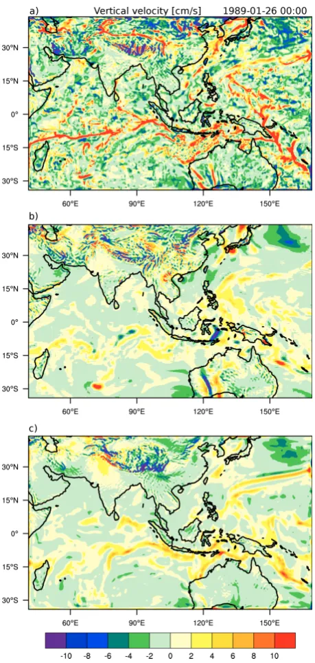
Figure 3 shows the fiday forecasts of the vertical ve-locities with starting date 21 January 1989. Again the zero-day forecast from 26 January (for LM) is used for verifi-cation. For the preparation of this initial field, see the LM model documentation (Steppeler et al., 2003 and references therein). Both forecasts and the verification show a band of rising motion in the tropical convergence zone, which in the east of the area is split into three branches. One of them is reaching far north into the vicinity of Japan. For the LM run the large-scale features are obscured by small-scale noise of rather high amplitude, which is present everywhere and is strongest over the high mountains and in the tropics, particu-larly downwind of Madagascar. These strong vertical veloc-ities are responsible for heavy rain with LM. The forecasted vertical velocities for LM verify much worse than those of LMZ as compared to the initial fields.

Some investigations were done concerning the noisy w field with LM and the associated heavy rain. These are sum-marised here without showing all corresponding diagrams. At the initial time LMZ and LM have very similarwfields, which for the LMZ forecast are evolving continuously and verify reasonably with thewfrom the analysed data. For LM large differences appear after the digital filter initialisation and are also seen in adiabatic runs. The digital filter initialisa-tion creates large-scale differences between LM and LMZ in the vertical velocity field, which are not localised near moun-tains. They occur for example in a large area downwind of Madagascar.

For diabatic runs the strong vertical velocities with LM create heavy precipitation, particularly in the tropical belt. This again creates even higher vertical velocities. Apparently the creation of the noisy structures over the whole model area after five days is caused by amplification of rising motion using the energy source of the warm tropical ocean. In the course of the five-day forecasts the high amplitude features of thew-field spread to the whole model area and cause in-creased rainfall rates everywhere.

Note that the model reaction is very different for precipi-tation and temperature. While the differences in precipiprecipi-tation are already large after the first day, the differences for tem-perature take about five days to build up (not shown).

The use of model initial fields for verification is problem-atic as the data assimilation derives fields also in areas with no observations. Therefore it is difficult to assess the accu-racy of the data used for verification. In particular the vertical velocity fieldwis obtained as a model field att=0 (Step-peler et al., 2003), with no direct measurements ofwbeing used. Therefore it is desirable to compare directly with ob-servations. Most readily available are precipitation data. As precipitation depends strongly on the vertical velocity, pre-cipitation verification can be seen as an indirect verification ofw. Here, we use the monthly, global gridded precipitation dataset from GPCC (Global Precipitation Climatology Cen-tre; V5, Schneider et al., 2013) with a grid resolution of 0.5◦ over land and from GPCP (Global Precipitation Climatology Project, V2.1, Huffman et al., 2009) with a grid resolution of 2.5◦ over the oceans as reference. To merge the data to a common grid, the GPCP precipitation over the oceans has been bi-linearly interpolated to the GPCC grid.

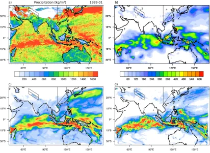
Figure 4 shows the accumulated precipitation for the LM, the LMZ and the CLM forecasts and the observations for the whole month of January 1989. The results from LMZ are almost everywhere more accurate than those from LM, with the latter being generally double the observed values. This again highlights the error in the old LM version resulting in much too high convective precipitation in the tropics.

(5)

J. Steppeler et al.: Forecasts covering one month using a cut-cell model 879

Fig. 2. (a)Temperature for the 5 day forecast from 1 January 1989 of level 20 for the terrain-following model LM (left), the cut-cell model LMZ (right) and the 0 day forecast from 6 January 1989 (“verification”, middle);(b–f)as(a), for dates 6, 11, 16, 21, 26 January. The black box in the top left corner denotes the area (T) used to calculate the temperature biases.

Fig. 2. (a) Temperature for the five-day forecast from 1 January 1989 of level 20 for the terrain-following model LM (left), the cut-cell model LMZ (right) and the zero-day forecast from 6 January 1989 (“verification”, middle); (b–f) as (a), for dates 6, 11, 16, 21, 26 January. The black box in the top left corner denotes the area (T) used to calculate the temperature biases.

at some places better for CLM than for LMZ. However, de-spite the lack of these improvements in the LMZ, the cut-cell model performs better than the CLM at some places, as can be seen from the precipitation biases given in Table 1. Forecast differences in favour of CLM are a tendency of the LMZ to predict light rain in areas which are dry. While CLM correctly produces extended areas of no precipitation, LMZ often produces light rain for such locations. This concerns parts of the Arabian Peninsula, India and Australia. This is a known error of older models and the expression “Socialist precipitation” has been coined for this. This clearly indicates that for operational applications the physics of LMZ needs to be modernised.

The rain produced south of the Caspian Sea is better with CLM as well. However, when a feature over land is pre-dicted both by LMZ and CLM, its position and shape is of-ten better with LMZ as for instance the banded structure of

precipitation south of the Himalayas and precipitation over Sri Lanka and Thailand, which are dry with CLM.

The largest differences are in the target area downwind of the Himalayas: southeastern China, Korea and Japan. The LMZ gives a better distribution of precipitation as compared to CLM. The precipitation is correctly concentrated in the south of China. Korea and Taiwan get precipitation and the rain over Japan is concentrated in the west of the country. These are differences involving a large area and they indicate that the mathematically more correct treatment of mountains with the LMZ has a considerable impact for prediction and climate simulation purposes. It is interesting that over dry ar-eas in Arabia and India the vertical velocity is negative for LMZ and LM. This again may be seen as an indication that the LMZ model needs an improvement of the physics scheme such as the changes leading from LM to CLM.

(6)

8 J. Steppeler et al.: Forecasts covering one month using a cut-cell model

Fig. 3. (a)Vertical velocitywfor level 20 of the five-day forecast from 21 January 1989 for the terrain-following model LM;(b)as

(a), for the 0 day forecast from 26 January (“verification”);(c)as

(a), for the cut-cell model LMZ.

Fig. 3. (a) Vertical velocitywfor level 20 of the five-day forecast from 21 January 1989 for the terrain-following model LM; (b) as (a), for the zero-day forecast from 26 January (“verification”); (c) as (a), for the cut-cell model LMZ.

the amplitudes for the tropical precipitation are still some-what too high for both LMZ and CLM, with the maximum reaching often 600 mm, where 400 to 500 mm are observed. Mostly, the overestimation is higher in LMZ than in CLM. However, east of the Philippines LMZ correctly predicts strong precipitation on the sea and immediately at the coast, while CLM has the precipitation a bit away from the coast.

The dry areas of the ocean are too large with CLM and the extension of precipitation into the Arabian Sea is better with LMZ. Further, the tropical precipitation belt is smoother with LMZ, which appears to be correct. However, observations over the oceans are known to include biases (Huffman et al., 2009) and are available at low resolution only (2.5◦ in this case), resulting in smooth fields when interpolated to a finer resolution.

The authors want to emphasise that the present study is still an impact study. For a proper evaluation of the cut-cells method, a larger sample of simulations and mesoscale res-olution is necessary. Currently, the authors aim to run 100 five-day forecasts using about 7 km resolution. The analysis of these simulations will include more quantitative verifica-tion. However, some simple scores have been computed to give quantitative meaning to the model differences. The areas for the computation were selected as places where the posi-tion of features was different in the forecasts and are shown in Figs. 2 and 4. For precipitation we extracted the bias for four areas lying in the shoulder of the Himalayas and east-ern China, and for temperature an area close to Mongolia has been chosen. The locations for the computation of the tem-perature anomaly correlations were selected in the lee area of the mountains, where the impact of cut cells is expected to be strongest.

The bias is calculated as Bias(model)=sim−ref, where sim are the model values and ref the reference values. For precipitation the mean is taken over the areas shown in Fig. 4. For temperature the mean is taken over the area shown in Fig. 2 for each of the six five-day forecasts and over the single time values. The anomaly correlation is calculated as

Corr(model)= 6 P

t=1

simt−sim reft−ref

s 6 P

t=1

simt−sim 2P6

t=1

reft−ref 2

.

To summarise, the positive impact for bias and anomaly correlation is in favour of the LMZ for all selected locations as can be seen in Tables 1 and 2. This improvement is present even in comparison with the state-of-the-art model CLM. Note that no quantitative comparison with the LM model was done for precipitation, as the LM precipitation is too high al-most everywhere.

4 Conclusions

(7)

J. Steppeler et al.: Forecasts covering one month using a cut-cell model 881

Fig. 4. (a)

The forecasted accumulated precipitation for the whole January 1989 using the terrain-following model LM;

(b)

as

(a)

, observed

according to the GPCC (land) and GPCP (ocean) dataset;

(c)

as

(a)

, for the cut-cell model LMZ;

(d)

as

(a)

, for the terrain-following model

CLM in its current version. For

(c)

and

(d)

, the same colour scheme as for

(b)

was used. The lines and the numbers 1 to 4 in

(b)

denote the

areas used to calculate the precipitation biases.

Fig. 4. (a) The forecasted accumulated precipitation for the whole January 1989 using the terrain-following model LM; (b) as (a), observed according to the GPCC (land) and GPCP (ocean) datasets; (c) as (a), for the cut-cell model LMZ; (d) as (a), for the terrain-following model CLM in its current version. For (c) and (d), the same colour scheme as for (b) was used. The lines and the numbers 1 to 4 in (b) denote the areas used to calculate the precipitation biases.

Table 2. Temperature anomaly correlations for LMZ and LM for selected locations.

City name location Corr (LMZ) Corr (LM)

Beijing 40◦N, 117◦E 0.80 0.16 Baoutu 41◦N, 110◦E 0.83 0.60 Yinchouan 38◦N, 105◦E 0.90 0.24 Gan Ze 33◦N, 100◦E 0.78 0.14

Xian 34◦N, 108◦E 0.55 0.34

the LM having large differences to the analysis. As shown for shorter forecasts in Stal06, the vertical velocities and precipi-tation are more realistic for the LMZ model, when compared to the control model LM. The small improvements of tem-perature and wind forecasts reported in Stal06 become more substantial after five days. Over large areas the temperatures and winds are improved, when using the analysed fields as verification. As the control model has a problem for tropical forecasts, the up to date CLM was used for comparison as well. The CLM differs from the LMZ model by improve-ments such as error corrections and tuning of the physics

scheme (see, e.g. Hollweg et al., 2008). These desirable im-provements are not yet implemented in the LMZ. In spite of this, the LMZ shows a better localisation of precipitation, even though in other aspects the CLM model gives better pre-cipitation forecasts.

Acknowledgements. The first author thanks NCAR for support of this work. The forecasts were done on the NCAR bluefire computer and visits of the first author to Boulder were financed by NCAR. ERA-interim data were provided by the European Centre for Medium-Range Weather Forecasts.

Edited by: H. Weller

References

Dobler, A.: A 2-D Finite Volume Non-Hydrostatic Atmospheric Model-Implementation of Cut Cells and Further Improvements, Diploma thesis, ETH Z¨urich, 2005.

(8)

Ensemble Simulations over Europe with the Regional Climate Model CLM Forced with IPCC AR4 Global Scenarios, Tech. Rep. 3, SGA-ZMAW Hamburg, 2008.

Huffman, G. J., Adler, R. F., Bolvin, D. T., and Gu, G.: Improv-ing the global precipitation record: GPCP version 2.1., Geophys. Res. Lett., 36, L17808, doi:10.1029/2009GL040000, 2009. Kessler, E.: On the Distribution and Continuity of Water Substance

in Atmospheric Circulations, Meteorol. Monogr., Am. Meteorol. Soc., Boston, Mass, 10, 84 pp., 1969.

Lock, S. J.: Development of a New Numerical Model for Study-ing Atmospheric Dynamics, Ph. D. thesis, University of Leeds, 158 pp., 2008.

Ritter, B. and Geleyn, J. F.: A comprehensive radiation scheme for numerical weather prediction models with potential applications in climate simulations, Mon. Weather Rev., 120, 303–325, 1992. Rockel, B. and Geyer, B.: The performance of the regional climate model CLM in different climate region, based on the example of precipitation, Meteorol. Z., 17, 487–498, 2008.

Schneider, U., Becker, A., Finger, P., Meyer-Christoffer, A., Ziese, M., and Rudolf, B.: GPCC’s new land surface precipita-tion climatology based on quality-controlled in situ data and its role in quantifying the global water cycle, Theor. Appl. Clim., 1–26, doi:10.1007/s00704-013-0860-x, 2013.

Schrodin, E. and Heise, E.: A new multi-layer soil model, COSMO Newsletter 2, 2002, available at http://www.cosmo-model.org/content/model/documentation/ newsLetters/newsLetter02/default.htm (21 June 2013), 2002. Seifert, A. and Crewell, S.: A revised cloud microphysical

parame-terization for operational numerical weather prediction using the COSMO model, 15th International Conference on Clouds and Precipitation ICCP 2008, Cancun, Mexico, 7–11 July 2008, 6 pp., 2008.

Steppeler, J., Bitzer, H. W., Minotte, M., and Bonaventura, L.: Non-hydrostatic atmospheric modelling using a z-coordinate repre-sentation, Mon. Weather Rev., 130, 2143–2149, 2002.

Steppeler, J., Doms, G., Sch¨attler, U., Bitzer, H. W., Gassmann, A., Damrath, U., and Gregoric, G.: Meso gamma scale forecasts by nonhydrostatic model LM, Meteorol. Atmos. Phys., 82, 75–96, 2003.

Steppeler, J., Bitzer, H. W., Janjic, Z., Sch¨attler, U., Prohl, P., Gjert-sen, U., Torrisi, L., Parfinievicz, J., Avgoustoglou, E., and Dam-rath, U.: Prediction of clouds and rain using az-coordinate non-hydrostatic model, Mon. Weather Rev., 134, 3625–3643, 2006. Steppeler, J., Park, S. -H., and Dobler, A.: A 5-day hindcast

exper-iment using a cut cell z-coordinate model, Atoms. Sci. Let., 12, 340–344, 2011.

Tiedtke, M.: A comprehensive mass flux scheme for cumulus pa-rameterization in large-scale models, Mon. Weather Rev., 117, 1779–1800, 1989.

Walko, R. L. and Avissar, R.: The ocean-land atmosphere model (OLAM). Part 2: Formulation and tests of the nonhydrostatic dy-namic core, Mon. Weather Rev., 136, 4045–4062, 2008. Yamazaki, H. and Satomura, H.: Vertically combined shaved cell

model in az-coordinate nonhydrostatic atmospheric model, At-mos. Sci. Lett., 9, 171–175, 2008.