www.geosci-model-dev.net/8/1595/2015/ doi:10.5194/gmd-8-1595-2015
© Author(s) 2015. CC Attribution 3.0 License.
A size-composition resolved aerosol model for simulating the
dynamics of externally mixed particles: SCRAM (v 1.0)
S. Zhu, K. N. Sartelet, and C. Seigneur
CEREA, joint laboratory Ecole des Ponts ParisTech – EDF R&D, Université Paris-Est, 77455 Champs-sur-Marne, France Correspondence to: S. Zhu ([email protected])
Received: 17 October 2014 – Published in Geosci. Model Dev. Discuss.: 20 November 2014 Revised: 30 April 2015 – Accepted: 5 May 2015 – Published: 1 June 2015
Abstract. The Size-Composition Resolved Aerosol Model (SCRAM) for simulating the dynamics of externally mixed atmospheric particles is presented. This new model classi-fies aerosols by both composition and size, based on a com-prehensive combination of all chemical species and their mass-fraction sections. All three main processes involved in aerosol dynamics (coagulation, condensation/evaporation and nucleation) are included. The model is first validated by comparison with a reference solution and with results of sim-ulations using internally mixed particles. The degree of mix-ing of particles is investigated in a box model simulation us-ing data representative of air pollution in Greater Paris. The relative influence on the mixing state of the different aerosol processes (condensation/evaporation, coagulation) and of the algorithm used to model condensation/evaporation (bulk equilibrium, dynamic) is studied.
1 Introduction
Increasing attention is being paid to atmospheric particu-late matter (PM), which is a major contributor to air pol-lution issues ranging from adverse health effects to visibil-ity impairment (EPA, 2009; Pascal et al., 2013). Concentra-tions of PM2.5 and PM10 are regulated in many countries,
especially in North America and Europe. For example, reg-ulatory concentration thresholds of 12 and 20 µg m−3 have been set for PM2.5annual mass concentrations in the United
States and Europe, respectively. Furthermore, particles influ-ence the Earth’s energy balance and global climate change (Myhre et al., 2013).
Three-dimensional chemical-transport models (CTM) are often used to study and forecast the formation and
distribu-tion of PM. The size distribudistribu-tion of particles is often discre-tised into sections (e.g. Gelbard and Seinfeld, 1980; Zhang et al., 2004; Sartelet et al., 2007) or approximated by log-normal modes (e.g. Whitby and McMurry, 1997; Binkowski and Roselle, 2003). Moreover, CTM usually assume that particles are internally mixed, i.e. each size section or log-normal mode has the same chemical composition, which may vary in space and time.
The internal-mixing assumption implies that particles of the same diameter (or in the same size section or log-normal mode) but originating from different sources have undergone sufficient mixing to achieve a common chemical composition for a given model grid cell and time. Although this assump-tion may be realistic far from emission sources, it may not be valid close to emission sources where the composition of new emitted particles can be very different from either back-ground particles or particles from other sources. Usually, in-ternally and exin-ternally mixed particles are not differentiated in most measurements, which may be size-resolved (e.g. cas-cade impactors) but not particle specific (McMurry, 2000). The use of mass spectrometers for individual particle analy-sis has shed valuable information on the chemical composi-tion of individual particles. Consequently, there is a growing body of observations indicating that particles are mostly ex-ternally mixed (e.g. Hughes et al., 2000; Mallet et al., 2004; Healy et al., 2012; Deboudt et al., 2010).
the internal mixing assumption). By influencing the hygro-scopic characteristics of particles, the mixing state also in-fluences the formation of secondary organic aerosols (SOA), because condensation/evaporation differs for species that are hydrophilic and/or hydrophobic (Couvidat et al., 2012). As the particle wet diameter is strongly related to the hygro-scopic properties of particles, the mixing state also impacts particle wet diameters and the number of particles that be-come cloud condensation nuclei (CCN), because the activa-tion of particles into CCN is strongly related to the parti-cle wet diameter (Leck and Svensson, 2015). By influenc-ing CCN, the mixinfluenc-ing state also affects aerosol wet removal and thus the aerosol spatial/temporal distribution. Besides, the mixing state influences the particle optical properties, which depend on both the particle size distribution (wet di-ameters) and composition (different chemical species pos-sess different absorption/scattering properties). Lesins et al. (2002) found that the percentage difference in the optical properties between an internal mixture and external mixture of black carbon and ammonium sulfate can be over 50 % for wet aerosols. The mixing state may also influence radiative forcing, as shown by Jacobson (2001), who obtained differ-ent direct forcing results between external and internal mix-ing simulations of black carbon.
Although CTM usually assume that particles are internally mixed, several models have been developed during the last sesquidecade to represent the external mixture of particles. A source-oriented model was developed by Kleeman et al. (1997) and Kleeman and Cass (2001) for regional modelling. In these models, each source is associated with a specific aerosol population, which may evolve in terms of size distri-bution and chemical composition, but does not mix with the other sources (i.e. particle coagulation is neglected). Riemer et al. (2009) modelled externally mixed particles using a stochastic approach. However, such an approach is compu-tationally expensive when the number of particle species is high. On the other hand, Stier et al. (2005) and Bauer et al. (2008) simulate externally mixed particles using modal aerosol models, where aerosol populations with different mixing states are represented by modes of different com-positions (soluble/mixed or insoluble/not mixed). Although these models may be computationally efficient, they may not model accurately the dynamics of mixing. To represent ex-ternally mixed particles independently of their sources and number concentrations, Jacobson et al. (1994) and Lu and Bowman (2010) considered particles that can be either inter-nally or exterinter-nally mixed (i.e. composed of a pure chemical species). Lu and Bowman (2010) used a threshold mass frac-tion to define whether the species is of significant concentra-tion. Jacobson (2002) expanded on Jacobson et al. (1994) by allowing particles to have different mass fractions. Similarly, Oshima et al. (2009) discretised the fraction of black car-bon in the total particle mass into sections of different chem-ical compositions. Dergaoui et al. (2013) further expanded on these modelling approaches by discretising the mass
frac-tion of any chemical species into secfrac-tions, as well as the size distribution (see Sect. 2.1.3 for details). Based on this dis-cretisation, Dergaoui et al. (2013) derived the equation for coagulation and validated their model by comparing the re-sults obtained for internal and external mixing, as well as by comparing both approaches against an exact solution. How-ever, processes such as condensation/evaporation and nucle-ation were not modelled.
This work presents the new Size-Composition Re-solved Aerosol Model (SCRAM), which expands on the model of Dergaoui et al. (2013) by including condensation/evaporation and nucleation processes. Sec-tion 2 describes the model. EquaSec-tions for the dynamic evolu-tion of particles by condensaevolu-tion/evaporation are derived. A thermodynamic equilibrium method may be used in SCRAM to compute the evolution of the particle chemical com-position by condensation/evaporation. Redistribution algo-rithms, which allow section bounds not to vary, are also sented for future 3-D applications. Model validation is pre-sented in Sect. 3 by comparing the changes in the particle size distribution due to condensational growth for both ex-ternally and inex-ternally mixed particles. Section 4 presents an application of the model with realistic concentrations over Greater Paris.
2 Model description
This section presents the aerosol general dynamic equations and the structure of the model. First, the formulation of the dynamic evolution of the aerosol size distribution and chem-ical composition by condensation–evaporation is introduced. Since it is necessary in 3-D CTM to maintain fixed size and composition section bounds, we present algorithms to re-distribute particle mass and number according to fixed sec-tion bounds. For computasec-tional efficiency, a bulk equilib-rium method, which assumes an instantaneous equilibequilib-rium between the gas and particle phases, is introduced. Finally, the overall structure of the model is described. In particular, the treatment of the different mixing processes to ensure the numerical stability of the model is discussed.
because this process not only largely influences the size dis-tribution of aerosols, but may also change the composition of particles significantly.
2.1 Condensation–evaporation algorithm
The focus of the following subsections is the formulation and implementation of the condensation/evaporation process. A Lagrangian approach is used to solve the equations of change for the mass and number concentrations, which are redis-tributed onto fixed sections through a redistribution algo-rithm (moving diameter, Jacobson, 1997). Equations are de-rived to describe the change with time of the mass concentra-tions of chemical species in terms of particle composiconcentra-tions. 2.1.1 Dynamic equation for condensation/evaporation Let us denotemi the mass concentration of speciesXi (1≤ i≤c) in a particle andx the vector representing the mass composition of the particlex=(m1, m2,· · ·, mc). Following
Riemer et al. (2009), the change with time of the number concentration n(x, t )(m−3µg−1) of multi-species particles by condensation/evaporation can be represented by the fol-lowing equation:
∂n ∂t = −
c X
i=1
∂(Iin) ∂mi
, (1)
whereIi (µg s−1) is the mass transfer rate between the gas
and particle phases for speciesXi. It may be written as
fol-lows: Ii=
∂mi
∂t =2π D
g
i dp f (Kn, αi)(c g i(t )
−Ke(dp) ceqi (x, t )), (2)
where Dig is the molecular diffusivity of condensing/evaporating species in the air, and dp and
cgi are the particle wet diameter and the gas-phase concen-tration of species Xi, respectively. Non-continuous effects
are described byf (Kn, αi)(Dahneke, 1983), which depends
on the Knudsen number,Kn=2dpλ (withλthe air mean free
path), and on the accommodation coefficientαi=0.5: f (Kn, αi)=
1+Kn
1+2Kn(1+Kn)/αi
. (3)
Ke(dp) represents the Kelvin effect (for ultra-fine
parti-cles, the curvature tends to inhibit condensation): Ke(dp)=exp
4σ v
p
R T dp
, (4)
with R the ideal gas constant, σ the particle surface ten-sion and vp the particle molar volume. The local
equi-librium gas concentration cieq is computed using the re-verse mode of the ISORROPIA V1.7 thermodynamic model
(Nenes et al., 1998) for inorganic compounds. In the cur-rent version of SCRAM, organic compounds are assumed to be at thermodynamic equilibrium with the gas phase and condensation/evaporation is computed as described in Sect. 2.2.
2.1.2 Dynamic equation as a function of mass fractions Following the composition discretisation method of Der-gaoui et al. (2013) (detailed in Sect. 2.1.3), each particle is represented by a vectorp=(f, m), which contains the mass fraction vector f =(f1, f2, . . ., f(c−1)) of the first (c−1)
species and the total massm=Pc i=1mi.
In Eq. (1), the chemical composition of particles is de-scribed by the vector x, which contains the mass concen-tration of each species. After the change of variable through a[c×c] Jacobian matrix from n(x, t ) to n(¯ p, t ) (see Ap-pendix A for detail), Eq. (1) becomes
∂n¯
∂t = − (c−1)
X
i=1
∂(Hin)¯
∂fi
−∂(I0n)¯
∂m , (5)
withI0=Pci=1Ii,Hi =∂f∂ti. Asfi =mmi is the mass fraction
of species (or group of species)Xi, we may write Hi =
1 m
∂mi ∂t −
mi m2
∂m ∂t =
Ii−fiI0
m . (6)
The change with time ofqi=n mi, the mass
concentra-tion of speciesXi, can be expressed as follows: ∂qi
∂t = ∂n ∂tmi+
∂mi
∂t n. (7)
After the change of variables fromqi(x, t )toq¯i(p, t )(see
Appendix A), Eq. (7) becomes ∂q¯i
∂t = −m fi ∂n¯
∂t + ¯n Ii. (8)
2.1.3 Discretisation
As SCRAM is a size-composition resolved model, both par-ticle size and composition are discretised into sections, while the numbers and bounds of both size and composition sec-tions can be customised by the user. The particle mass dis-tributionQ[mmin, mmax]is first divided intoNbsize sections
[m−k, m+k](k=1, . . ., Nb andm+k−1=m −
k), defined by
dis-cretising particle diameters[dmin, dmax]withdminanddmax,
the lower and upper particle diameters, respectively, and mk=
π ρ dk3
6 . For each of the first(c−1)species or species
groups, the mass fraction is discretised into Nf fraction
ranges. Thehth fraction range is represented by the range Fh+−= [f
−
h , f
+
h ]wheref
+
h−1=f −
h ,fmin=0 andfmax=1.
Within each size section k, particles are categorised into Np composition sections, which are defined by the valid
The gth composition section can be represented by Pg= (Fg1+−, Fg2
+
−, . . ., Fgc−1 +
−). Given the mass fraction
discreti-sation, those composition sections are automatically gener-ated by an iteration on all possible combinations (Nf(c−1)) of
the(c−1)species andNffraction ranges. Only the
compo-sition sections that satisfyP(c−1) i=1 Fgi
−
61 are kept.
The particle mass distribution is discretised into(Nb×Np)
sections. Each sectionj (j=1, . . ., Nb×Nc) corresponds to
a size sectionk(k=1, . . ., Nb) and to a composition section g=(g1, . . ., g(c−1))withg=1, . . ., Np,gh=1, . . ., Nfwith
h=1, . . ., (c−1). The total concentrationQji of speciesiin thejth section can be calculated as follows:
Qji =
m+k Z
m−k fg+
1 Z
fg−1 . . .
f+
g(c−1) Z
fg(c−−1)
¯
qi(m, fg1, . . ., fg(c−1))
dmdfg1. . .dfg(c−1). (9)
Similarly, the number concentrationNj of thejth section may be written as follows:
Nj=
m+k Z
m−k f+
g1 Z
fg−1 . . .
f+
g(c−1) Z
fg(c−−1)
¯
n(m, fg1, . . ., fg(c−1))
dmdfg1. . .dfg(c−1). (10)
After a series of derivations (see Appendix B for details), we obtain the time derivation of Eq. (10):
∂Nj
∂t =0, (11)
as well as the time derivation of Eq. (9): ∂Qji
∂t =N j I
gi. (12)
Thus, in each section, the change with time of number and mass concentrations is given by Eqs. (11) and (12).
2.1.4 Numerical implementation
According to Debry and Sportisse (2006), the condensation/evaporation process may have character-istic timescales of different magnitudes, because the range of particle diameters is large. Such a feature induces strong stiffness of the numerical system. As suggested by Debry et al. (2007), the stiff condensation/evaporation equations are solved using the second-order Rosenbrock (ROS2) method (Verwer et al., 1999; Djouad et al., 2002).
In addition, potentially unstable oscillations may occur when a dramatic change of the particle pH occurs. To address this issue, a species flux electro-neutrality constraint (Pilinis et al., 2000; Debry et al., 2007) is applied in SCRAM to en-sure the numerical stability of the system.
2.1.5 Size and composition redistribution
By condensation/evaporation, the particles in each size tion may grow or shrink. Because the bounds of size sec-tions should be fixed for 3-D applicasec-tions, it is necessary to redistribute number and mass among the fixed size sec-tions during the simulation after condensation/evaporation. Similarly, the chemical composition also evolves by condensation/evaporation, and an algorithm is needed to identify the particle composition and redistribute it into the correct composition sections.
Two redistribution methods for size sections may be used in SCRAM: the HEMEN (Hybrid of Mass and Euler-Number) scheme of Devilliers et al. (2013) and the moving diameter scheme of Jacobson (1997). According to Devilliers et al. (2013), both redistribution methods may accurately re-distribute mass and number concentrations.
The HEMEN scheme divides particle size sections into two parts: the number is redistributed for sections of mean diameter lower than 100 nm and mass is redistributed for sections of mean diameter greater than 100 nm. The sec-tion mean diameters are kept constant and mass concen-trations are diagnosed for sections where number is redis-tributed, while number concentrations are diagnosed for sec-tions where mass is redistributed. The advantage of this scheme is that it is more accurate for number concentra-tions over the size range where number concentraconcentra-tions are the highest and more accurate for mass concentrations where mass concentrations are the highest. In SCRAM, the algo-rithm of Devilliers et al. (2013) was modified to take into account the fact that after condensation/evaporation, the di-ameter of a section may become larger than the upper bound of the next section. In that case, the mean diameter of the section after condensation/evaporation is used to diagnose in which fixed-diameter sections the redistribution is per-formed. This feature allows us to use larger time steps for condensation/evaporation before redistribution.
In the moving diameter method, although size sec-tion bounds are kept fixed, the representative diame-ter of each size section is allowed to vary. If, afdiame-ter condensation/evaporation, the diameter grows or shrinks outside section bounds, both the mass and number concen-trations of the section are redistributed entirely into the new size sections bounding that diameter.
The composition redistribution is applied first, followed by the size redistribution for each of the composition sections. 2.2 Bulk equilibrium and hybrid approaches
Bulk equilibrium methods assume an instantaneous ther-modynamic equilibrium between the gas and bulk-aerosol phases. For semi-volatile species, the mass con-centrations of both gas and bulk-aerosol phases after condensation/evaporation are obtained using the forward mode of ISORROPIA for inorganics and the H2O model (Couvidat et al., 2012) for organics. Because time integra-tion is not necessary, the computaintegra-tional cost is significantly reduced compared to the dynamic method. Weighting fac-tors W are designed to distribute the semi-volatile bulk-aerosol mass across the bulk-aerosol distribution (Pandis et al., 1993). In SCRAM, for each semi-volatile species i, we re-distribute the bulk aerosol evaporating or condensing mass, δQi=Qafter bulk eq.i −Qbefore bulk eq.i , between the sectionsj,
using factors that depend on the ratio of the mass transfer rate in the aerosol distribution (Eq. 2). Because of the bulk equilibrium assumption, the driving force of(cgi −Keceqi )is
assumed to be the same for all size and composition sections, and the weighting factors are as follows.
Wij= Nj d
j
pf (Kn, αi)
PNs
k=1Nk dpkf (Kn, αi)
, (13)
whereNj is the number concentration of sectionj anddpj
is the particle wet diameter of sectionj. In case of evapora-tion, these weighting factors may not be appropriate, as they may lead to over-evaporation of some species in some sec-tions, i.e.Qji after bulk eq.=Qbefore bulk eq.i +δQi×Wij<0. In
the case of over-evaporation, we use a weighting scheme that redistributes the total bulk aerosol mass rather than the bulk aerosol evaporating or condensing mass
Wij= Q
j i
PNs
k=1Qki
(14)
andQji after bulk eq.=Qafter bulk eq.i ×Wij.
In fact, due to their larger ratios between surface area and particle mass, small particles may reach thermodynamic equilibrium much faster than large particles. Particles of di-ameters larger than 1 µm could require hours or even days to achieve equilibrium (Wexler and Seinfeld, 1990), which makes the bulk equilibrium assumption inappropriate for them. In order to maintain both the computational efficiency of the equilibrium method and the accuracy of the dynamic one, a hybrid method is adopted in SCRAM based on the work of Capaldo et al. (2000) and Debry and Sportisse (2006). This method uses the equilibrium method for small particles (dp<1 µm) and uses the dynamic method to
calcu-late the mass transfer for larger particles.
2.3 Overall time integration and operator splitting in SCRAM
In order to develop a system that offers both computational efficiency and numerical stability, we perform operator split-ting for changes in number and mass concentrations with time due to emission, coagulation, condensation/evaporation and nucleation, as explained below.
Emissions are first evaluated with an emission time step, which is determined by the characteristic timescales of emissions obtained from the ratio of emission rates to aerosol concentrations. The emission time step evolves with time to prevent adding too much emitted mass to the system within one time step. Within each emission time step, coagulation and condensation/evaporation/nucleation are solved, and the splitting time step between coagula-tion and condensacoagula-tion/evaporation/nucleation is forced to be lower than the emission time step. Time steps are obtained from the characteristic time steps of coagu-lation (tcoag) and condensation/evaporation/nucleation
(tcond). The larger of the time steps tcoag and tcond
determines the time step of splitting between co-agulation and condensation/evaporation/nucleation. As coagulation is usually the slower process, the change due to coagulation is first calculated over its time step. Then, condensation/evaporation/nucleation are solved simultaneously. The change due to condensation/evaporation/nucleation is calculated, us-ing time sub cycles, startus-ing with the sub time steptcond. The
next sub time step for condensation/evaporation/nucleation is estimated based on the difference between the first-and second-order results provided by the ROS2 solver. Redistribution is computed after each time step of splitting of coagulation and condensation/evaporation/nucleation.
When the bulk thermodynamic equilibrium approach is used to solve condensation/evaporation, coagulation and then nucleation are solved after each emission time step. The resolution is done as previously explained, except that the dy-namic condensation/evaporation solver is disabled: sub time steps are used to solve coagulation and nucleation during one emission time step. Condensation/evaporation is then solved using the bulk equilibrium approach and the redistribution process is applied after the bulk equilibrium algorithm.
size sections: emissions are solved followed by coagulation and condensation/evaporation/nucleation. As in the fully dynamic approach, redistribution is applied after dynamic condensation/evaporation.
3 Model validation
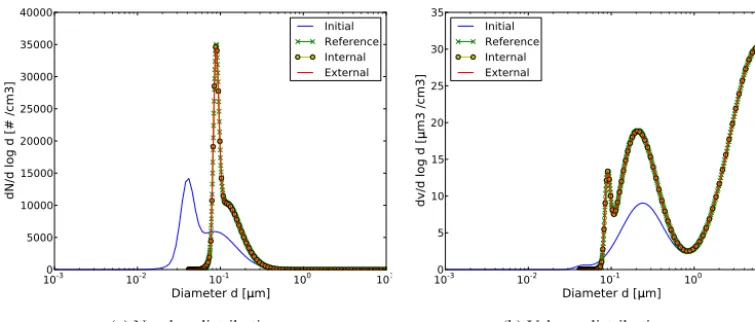
To validate the model, the change with time of internally and externally mixed aerosol models is compared. The simula-tions use initial condisimula-tions for number and mass concentra-tions that are typical of a regional haze scenario, with con-stant sulfuric acid vapour source that gives a sulfuric acid condensation rate of 5.5 µm3cm−3per 12 h (Seigneur et al., 1986; Zhang et al., 1999).
Simulations were conducted for 12 h at a temperature of 298 K and a pressure of 1 atm. The original reference sim-ulation (Seigneur et al., 1986; Zhang et al., 1999) was first reproduced for internally mixed sulfate particles (redistribu-tion is not applied). For the sake of comparison between in-ternally and exin-ternally mixed simulations, half of the parti-cles were assumed to consist of sulfate (species 1) and the other half of another species of similar physical properties as sulfate (species 2). For internal mixing, the initial parti-cles are all 50 % species 1 and 50 % species 2; and for ex-ternal mixing, half of the initial particles are 100 % species 1 and the other half are 100 % species 2. As both species have the same physical properties, for any given size section, the sum over all composition sections of number and mass concentrations of externally mixed particles should equal the number and mass concentrations of the internally mixed par-ticles. Particles were discretised into 100 size sections and 10 composition sections for the externally mixed case. Fig-ure 1 shows the initial and final distributions for the number and volume concentrations as a function of particle diame-ters. Both the internally mixed and externally mixed results are presented in Fig. 1, along with the reference results of Zhang et al. (1999) (500 size sections were used in the orig-inal reference simulation). For the externally mixed simula-tion, the results were summed up over composition sections to obtain the distributions as a function of particle diameter. As expected, an excellent match is obtained between inter-nal and exterinter-nal mixing distributions, with an almost 100 % Pearson’s correlation coefficient. Furthermore, the accuracy of the SCRAM algorithm is proved by the excellent match between the results of these simulations and the reference simulation of Zhang et al. (1999). In order to investigate the influence of the composition resolution on simulation results, two additional tests are conducted using 2 and 100 composi-tion bins. The mean mass fraccomposi-tion of species 1 is computed for all particles within each size section, as well as their stan-dard deviations. Figure 2 shows the size distribution of these statistics. The mean mass fraction is barely affected by the different composition resolutions, as the condensation rate of sulfate is independent of the particle compositions.
How-ever, a different composition resolution does lead to differ-ent standard deviation distributions, as only particles with a larger fraction difference (d >0.2 µm for 2 compositions and d >0.09 µm for 10 compositions) can be distinguished from each other under coarser composition resolutions.
Using the same initial conditions and sulfuric acid conden-sation rate, a second comparison test was performed, with both coagulation and condensation occurring for 12 h. As the coagulation algorithm requires size sections to have fixed bounds (Dergaoui et al., 2013), size redistribution was ap-plied for both the internally and externally mixed cases using the HEMEN method. As in the first comparison test, Fig. 3 shows that there is an excellent match between the internally and externally mixed distributions as a function of particle di-ameter (no reference simulation was available for these simu-lations). This test validates the algorithm of SCRAM to sim-ulate jointly the coagulation and condensation of externally mixed particles.
The mixing states of both internally and externally mixed particles at the end of the simulations of the second test are shown in Fig. 4. Sulfuric acid condenses to form particulate sulfate (species 1). During the simulation, pure species 2 par-ticles mix with pure sulfate parpar-ticles by coagulation and con-densation of sulfuric acid. Figure 4 shows that, at the end of the simulation, the sulfate mass fraction is greater for par-ticles of lower diameters, because the condensation rate is greater for those particles. Particles with diameters greater than 10 µm remain unmixed. However, the external mixing state provides a more detailed mixing map, from which it is possible to distinguish mixed particles from unmixed ones and to trace the origin of each particle. In this test case where the effect of condensation dominates that of coagulation, most mixed particles are originally pure species 2 particles coated with newly condensed sulfuric acid (Fig. 4).
4 Simulation with realistic concentrations
To test the impact of external mixing on aerosol concentra-tions, simulations of coagulation, condensation/evaporation and nucleation were performed with SCRAM using realistic ambient concentrations and emissions extracted from a sim-ulation performed over Greater Paris for July 2009 during the MEGAPOLI (Megacities: Emissions, urban, regional and Global Atmospheric POLution and climate effects, and Inte-grated tools for assessment and mitigation) campaign (Cou-vidat et al., 2013).
4.1 Simulation set-up
10-3 10-2 10-1 100 101
Diameter d [ m]
0 5000 10000 15000 20000 25000 30000 35000 40000
dN/d log d [# /cm3]
Initial Reference Internal External
(a) Number distribution
10-3 10-2 10-1 100 101
Diameter d [m]
0 5 10 15 20 25 30 35
dv/d log d [
m3 /cm3]
Initial Reference Internal External
(b) Volume distribution
Figure 1. Simulation of condensation for hazy conditions: initial distribution and after 12 h.
10
-310
-210
-110
010
1Diameter d [
m]
0.0
0.2
0.4
0.6
0.8
1.0
Mass fraction of species 1 [0,1]
mean, 2 sections
mean, 10 sections
mean, 100 sections
std, 2 sections
std, 10 sections
std, 100 sections
Figure 2. Mean and standard deviations of species 1 mass fraction
as functions of particle diameter using 2, 10 and 100 composition sections.
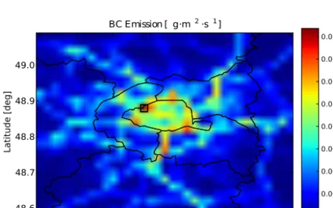
on 1 July 2009. The highest emission rate is located at the grid cell centre of longitude and latitude (2.28◦E, 48.88◦N), which was selected here to extract the SCRAM simulation input data for emissions, background gas and aerosol con-centrations, and initial meteorological conditions (tempera-ture and pressure). In the absence of specific information on individual particle composition, all initial aerosol concentra-tions extracted from the database were assumed to be 100 % mixed (i.e. aged background aerosols).
Simulations start at 02:00 UT (1 July 2009), i.e. just before the morning peak of traffic emissions, and last 12 h. As our simulations are 0D, the transport of gases and particles and the deposition processes are not taken into account. There-fore, emissions accumulate, potentially leading to unrealis-tically high concentrations. To avoid this artifact, the dura-tion of the emissions was limited to the first 40 min of
sim-ulation. This time duration is calculated using the average BC emission rate between 02:00 and 03:00 UT, so that BC emissions lead to an increase in BC concentrations equal to the difference between BC concentrations after and before the morning traffic peak, i.e. between 06:00 and 02:00 UT (Fig. 6). Besides, gas-phase chemistry (such as SOA forma-tion) is not included in SCRAM, and is expected to be solved separately using a gas-phase chemistry scheme. In the simu-lations of this work, SOA originate either from initial condi-tions or they are emitted as semi-volatile organic compounds during the simulation. They partition between the gas and the aerosol phases by condensation/evaporation.
10-3 10-2 10-1 100 101
Diameter d [m]
0 5000 10000 15000 20000 25000 30000 35000 40000
dN/d log d [# /cm3]
Initial Internal External
(a) Number distribution
10-3 10-2 10-1 100 101
Diameter d [m]
0 5 10 15 20 25 30 35
dv/d log d [
m3 /cm3]
Initial Internal External
(b) Volume distribution
Figure 3. Simulation of both coagulation and condensation for hazy conditions: initial distribution and after 12 h.
10-3 10-2 10-1 100 101
diameter [m]
0.0 0.1 0.2 0.3 0.4 0.5 0.6 0.7 0.8 0.9 1.0
species 1 mass fraction [0, 1]
0.00 6.00 12.00 18.00 24.00 30.00 36.00 42.00 48.00 54.00
[
g/m3]
(a) Internal mixing
10-3 10-2 10-1 100 101
diameter [ m]
0.0 0.1 0.2 0.3 0.4 0.5 0.6 0.7 0.8 0.9 1.0
species 1 mass fraction [0, 1]
0.00 6.00 12.00 18.00 24.00 30.00 36.00 42.00 48.00 54.00
[
g/m3]
(b) External mixing
Figure 4. Distribution after 12 h: particle mass concentration as a function of diameter and mass fraction of species 1.
2.0 2.1 2.2 2.3 2.4 2.5 2.6
Longitude [deg] 48.6
48.7 48.8 48.9 49.0
Latitude [deg]
BC Emission [ g·m¡ 2
·s¡1
]
0.000 0.003 0.006 0.009 0.012 0.015 0.018 0.021 0.024
Figure 5. BC emissions over Greater Paris at 02:00 UT, 1 July 2009.
BiNGA, NIT3, BiNIT, AnCLP, SOAlP, SOAmP, SOAhP, POAlP, POAmP and POAhP); the black carbon group (BC) contains only black carbon; and the dust group (DU) contains all the neutral particles made up of soil, dust and fine sand.
0 5 10 15 20 time (s)
1.0 1.5 2.0 2.5 3.0 3.5 4.0 4.5
M
[
u
g
/
m
3
]
BC
h UTC
Figure 6. Transport BC concentration profile of 1 July 2009.
mass conservation, and the composition section of the parti-cles would be chosen depending on this mass fraction.
In each group, water may also be present, although it is not considered when computing the mass fractions (it is cal-culated separately with the thermodynamic equilibrium mod-els).
The model memorises the relationship between each species index and group index, and it stores the mass con-centrations separately for each species within each size-composition section. The total mass concentration of each group is computed from the mass concentration of each species based on the species-group relations, allowing the computation of the mass fraction of each group.
4.2 Aerosol dynamics and mixing state
To understand how initial concentrations mix with emissions, four scenarios were simulated. In scenario (A), only emis-sions are taken into account in the simulation. Only coag-ulation is added to emissions in scenario (B), while only condensation/evaporation (C/E) is added to emissions in scenario (C). In scenario (D), emissions and all the aerosol dynamic processes are taken into account, including nucle-ation (however, no nuclenucle-ation occurred during the simulnucle-ation due to low sulfuric acid gas concentrations).
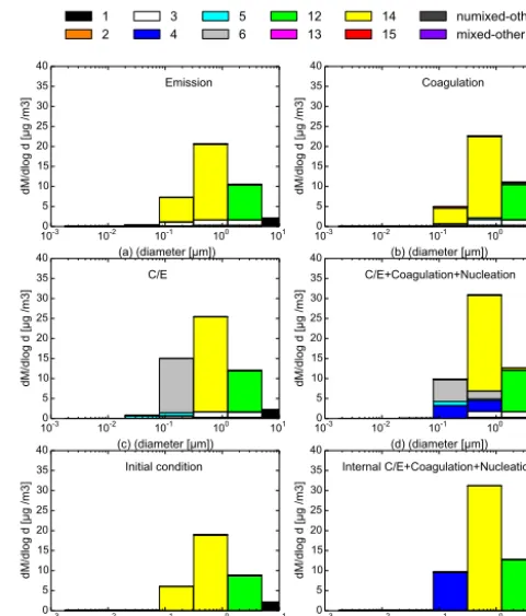
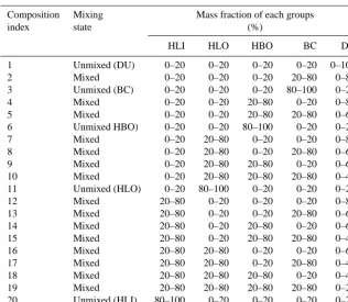
The mass and number distributions of each chemical com-position after 12 h of simulation are shown in Figs. 7 and 8 as a function of particle diameter, as well as their initial dis-tributions in sub-figure (e). Bars with greyscale represent un-mixed particles, while bars with colours are un-mixed particles. Each bar corresponds to a chemical composition index (CI). However, any CI with a small number or mass concentrations are not really visible from the plot, so they are regrouped into mixed-other (for mixed CI) and unmixed-other (for unmixed CI) in the plot. The chemical compositions and the CI value associated with colour bars are listed in Table 1. All emitted particles are unmixed: CI 1 (100 % DU) into size section (4– 6), CI 3 (100 % BC) into size section (3–6). So any mixed
10-3 10-2 10-1 100 101
(a) (diameter [µm])
0 5 10 15 20 25 30 35 40
dM/dlog d [µg /m3]
Emission
10-3 10-2 10-1 100 101
(b) (diameter [µm])
0 5 10 15 20 2530 35 40
dM/dlog d [µg /m3]
Coagulation
10-3 10-2 10-1 100 101
(c) (diameter [µm])
0 5 10 15 20 25 30 35 40
dM/dlog d [µg /m3]
C/E
10-3 10-2 10-1 100 101
(d) (diameter [µm])
0 5 10 15 20 25 30 35 40
dM/dlog d [µg /m3]
C/E+Coagulation+Nucleation
10-3 10-2 10-1 100 101
(e) (diameter [µm])
0 5 10 15 20 25 30 35 40
dM/dlog d [µg /m3]
Initial condition
10-3 10-2 10-1 100 101
(f) (diameter [µm])
0 5 10 15 20 25 30 35 40
dM/dlog d [µg /m3]
Internal C/E+Coagulation+Nucleation
1
2 34 56 1213 1415 numixed-othermixed-other
Figure 7. Result mass distributions of externally mixed
parti-cles as a function of particle diameter for the different chemi-cal compositions for six different simulation scenarios: (a)
emis-sion only; (b) emisemis-sion+coagulation; (c) emission+C/E; (d)
emis-sion+coagulation+C/E+nucleation; (e) initial condition; and (f)
internal mixing result.
particles represented in sub-figure (a) of Figs. 7 and 8 are due to initial condition instead of emissions. Besides, emis-sions also involve gas-phase POA and H2SO4, which can not
be observed in sub-figure (a) of Figs. 7 and 8 as they has no interaction with particle phase under scenario (A). Organic vapours which may lead to the production of SOA are not included in the emissions, while a certain concentration of such vapours is defined within the initial condition.
As shown by the simulation of scenario (A), emissions lead to high number concentrations of BC in the sections of low diameters (mostly below 0.631 µm) and to high mass concentrations of dust and BC in the sections of high diame-ters (mostly above 0.631 µm).
Table 1. 20 externally mixed particle compositions.
Composition Mixing Mass fraction of each groups
index state (%)
HLI HLO HBO BC DU
1 Unmixed (DU) 0–20 0–20 0–20 0–20 0–100
2 Mixed 0–20 0–20 0–20 20–80 0–80
3 Unmixed (BC) 0–20 0–20 0–20 80–100 0–20
4 Mixed 0–20 0–20 20–80 0–20 0–80
5 Mixed 0–20 0–20 20–80 20–80 0–60
6 Unmixed HBO) 0–20 0–20 80–100 0–20 0–20
7 Mixed 0–20 20–80 0–20 0–20 0–80
8 Mixed 0–20 20–80 0–20 20–80 0–60
9 Mixed 0–20 20–80 20–80 0–20 0–60
10 Mixed 0–20 20–80 20–80 20–80 0–40
11 Unmixed (HLO) 0–20 80–100 0–20 0–20 0–20
12 Mixed 20–80 0–20 0–20 0–20 0–80
13 Mixed 20–80 0–20 0–20 20–80 0–60
14 Mixed 20–80 0–20 20–80 0–20 0–60
15 Mixed 20–80 0–20 20–80 20–80 0–40
16 Mixed 20–80 20–80 0–20 0–20 0–60
17 Mixed 20–80 20–80 0–20 20–80 0–40
18 Mixed 20–80 20–80 20–80 0–20 0–40
19 Mixed 20–80 20–80 20–80 20–80 0–20
20 Unmixed (HLI) 80–100 0–20 0–20 0–20 0–20
Table 2. Mixing state after 12 h simulation.
Process No Dynamic Coagulation C/E C/E+Coag+Nucl
scenario (A) scenario (B) scenario (C) scenario (D)
Mixed particle number (%) 42 79 48 51
Mixed particle mass (%) 83 85 64 76
14 size section 4 particles with CI 3 size section 3 particles, or between two CI 15 size section 3 particles.
As shown by the simulation of scenario (C), C/E leads to high mass and number concentrations of unmixed HBO (CI 6 – mass fraction of HBO (81.2 %) above 80 % (ex-act mass fr(ex-action of the dominant group will be specified within the parentheses right after the group name here af-ter)), increasing the amount of unmixed particles. Organic matter of low and medium volatilities is emitted in the gas phase following Couvidat et al. (2013). This organic matter condenses subsequently on well-mixed particles (CI 14 with mixed HLI (31 %) and HBO (41 %)), in sufficient amount to increase the mass fraction of HBO (81 %) to over 80 % and, therefore, transfer particles to the unmixed category CI 6 (these particles are not exactly unmixed since up to 20 % may correspond to HLI (10 %), but a finer composition reso-lution would be required to analyse their mixed characteris-tics). The condensation of organic matter on freshly emitted BC particles (CI 3) also occurs, as shown by the mixed BC
(26 %) and HBO (68 %) particles (CI 5) which appear in the third and fourth size sections.
As shown by comparing scenarios (A) and (B) and sce-narios (C) and (D), coagulation significantly reduces num-ber concentrations. The mass concentrations of fine particles (diameters lower than 0.631 µm) are also reduced. Further-more, the composition diversity increases. For example, as demonstrated by the difference between scenarios (C) and (D), newly mixed particles of CI 4 (between 20 and 80 % of HBO (78 % for size 4 and 73 % for size 5)) are formed by the coagulation of unmixed particles from CI 6 with others within the fourth and fifth size sections.
10-3 10-2 10-1 100 101
(a) (diameter [µm])
0 1e10 2e10 3e10 4e10 5e10
dN/dlog d [# /m3]
Emission
10-3 10-2 10-1 100 101
(b) (diameter [µm])
0 1e10 2e10 3e10 4e10 5e10
dN/dlog d [# /m3]
Coagulation
10-3 10-2 10-1 100 101
(c) (diameter [µm])
0 1e10 2e10 3e10 4e10 5e10
dN/dlog d [# /m3]
C/E
10-3 10-2 10-1 100 101
(d) (diameter [µm])
0 1e10 2e10 3e10 4e10 5e10
dN/dlog d [# /m3]
C/E+Coagulation+Nucleation
10-3 10-2 10-1 100 101
(e) (diameter [µm])
0 1e10 2e10 3e10 4e10 5e10
dN/dlog d [# /m3]
Initial condition
10-3 10-2 10-1 100 101
(f) (diameter [µm])
0 1e10 2e10 3e10 4e10 5e10
dN/dlog d [# /m3]
Internal C/E+Coagulation+Nucleation
1
2 34 56 1213 1415 numixed-othermixed-other
Figure 8. Result number distributions of externally mixed
parti-cles as a function of particle diameter for the different chemical compositions for six different simulation scenarios: (a) emission
only; (b) emission+coagulation; (c) emission+C/E; (d)
emis-sion+coagulation+C/E+nucleation; (e) initial condition; (f)
in-ternal mixing result.
dominating for large particles due to their low emissions and the short duration of the simulations.
The number/mass mixing percentages after emission only (scenario A) provide a baseline for the analysis of the three other scenarios. In scenario (A), 42 % (resp. 83 %) of the par-ticle number (resp. mass) originates from initial conditions and is mixed, while the remaining particles are due to emis-sions and are unmixed. The comparison of scenarios (A) and (B) shows that coagulation increases the mixing percentages, especially for small particles of high number concentrations. The mass mixing percentages decrease in scenario (C) be-cause the condensation of freshly emitted organic matter on large mixed particles leads to particles with a mass fraction of organic matter (HBO) higher than 80 %, i.e. unmixed. When all aerosol dynamic processes are taken into account (sce-nario D), only 51 % of particle number concentration and 76 % of particle mass concentration are mixed. The mixing percentages are greater than those of scenario (C), as mixing increases by coagulation, but the mass mixing percentage is lower than in scenario (A) (emissions only) because of the strong condensation of HBO emitted in the gas phase.
10-3 10-2 10-1 100 101
(a) (diameter [µm]) 0
5 10 15 20 25 30 35 40
dM/dlog d [µg /m3]
External C/E Bulkeq
10-3 10-2 10-1 100 101
(b) (diameter [µm]) 0
5 10 15 20 25 30 35 40
dM/dlog d [µg /m3]
Internal C/E Bulkeq
10-3 10-2 10-1 100 101
(c) (diameter [µm]) 0
5 10 15 20 25 30 35 40
dM/dlog d [µg /m3]
External C/E Hybrid
10-3 10-2 10-1 100 101
(d) (diameter [µm]) 0
5 10 15 20 25 30 35 40
dM/dlog d [µg /m3]
Internal C/E
1
2 34 56 1213 1415 numixed-othermixed-other
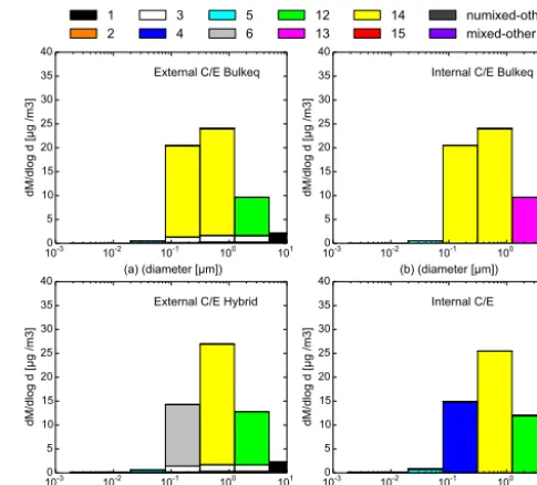
Figure 9. Result mass distributions of externally mixed particles
as a function of particle diameter for the different chemical com-positions for four different C/E simulation scenarios: (a) external bulk equilibrium; (b) internal bulk equilibrium; (c) external hybrid method; and (d) internal dynamic.
4.3 External versus internal mixing
To investigate the consequence of the internal mixing hy-pothesis, a simulation of scenario (D) (all aerosol dynamic processes are taken into account) is conducted by assuming all particles to be internally mixed. Externally and internally mixed 12 h simulations lead to a similar total aerosol mass concentration after 12 h (33.09 µg m−3 for internal mixing and 33.35 µg m−3 for external mixing) as well as to simi-lar total number concentrations (1.16×10¹⁰# m−3 for in-ternal mixing and 1.07×10¹⁰# m−3 for external mixing). The bulk mass concentrations of individual species are also similar, although external mixing leads to slightly lower ammonium concentrations (2.68 # m−3 versus 2.70 # m−3), slightly higher nitrate concentrations (3.19 # m−3 versus 3.03 # m−3) and higher chloride concentrations (0.36 # m−3 versus 0.25 # m−3). The size distributions for number and for individual species masses are also very similar in the internal and external mixing simulations.
10-3 10-2 10-1 100 101
(a) (diameter [µm])
0 1e10 2e10 3e10 4e10 5e10
dN/dlog d [# /m3]
External C/E Bulkeq
10-3 10-2 10-1 100 101
(b) (diameter [µm])
0 1e10 2e10 3e10 4e10 5e10
dN/dlog d [# /m3]
Internal C/E Bulkeq
10-3 10-2 10-1 100 101
(c) (diameter [µm])
0 1e10 2e10 3e10 4e10 5e10
dN/dlog d [# /m3]
External C/E Hybrid
10-3 10-2 10-1 100 101
(d) (diameter [µm])
0 1e10 2e10 3e10 4e10 5e10
dN/dlog d [# /m3]
Internal C/E
1
2 34 56 1213 1415 numixed-othermixed-other
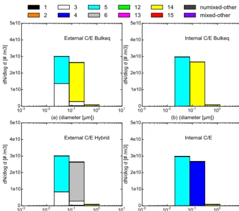
Figure 10. Result number distributions of externally mixed
parti-cles as a function of particle diameter for the different chemical compositions for four different C/E simulation scenarios: (a) ex-ternal bulk equilibrium; (b) inex-ternal bulk equilibrium; (c) exex-ternal hybrid method; and (d) internal dynamic.
are mostly hydrophobic organics (HBO 78 %) (CI 4) as in internal mixing, a large amount are unmixed particles (CI 6: HBO (82 %) between 80 and 100 %), and some are equally mixed with BC and hydrophobic organics (CI 5). In size sec-tion 5, as in the internal mixing simulasec-tion, mixed particles dominate (CI 14 – HLI 46 %, HBO 36 %), but many have a different composition (CI 4 and 5) and some are unmixed HBO 83 % (CI 6), BC 91 % (CI 3) and dust 90 % (CI 1). For particles in size section 6, particles are mixed particles of CI 12 (HLI 54 %,DU 29 %), while external mixing also shows that some particles are unmixed (BC 99 % (CI 3) and dust 98 % (CI 1)) and there are CI 14 (HLI 46 %, HBO 35 %) par-ticles that originated from size section 5 through coagulation. 4.4 Bulk equilibrium and hybrid approaches
Additional external mixing tests were conducted using the bulk equilibrium and hybrid approaches for C/E to evalu-ate both their accuracy and computational efficiency. In the hybrid approach, the lowest four sections are assumed to be at equilibrium (up to diameters of 0.1585 µm), whereas the other sections undergo dynamic mass transfer between the gas and particle phases.
The accuracy of these approaches is evaluated by compar-ing the mass and number distributions after 12 h simulations with the bulk equilibrium or the hybrid approaches to the mass and number distributions computed dynamically (see Figs. 9 and 10).
For externally mixed particles, the dynamic mass distri-bution is shown in Fig. 7c; the bulk equilibrium and hybrid
mass distributions are shown in Fig. 9a and c, respectively. The dynamic number distribution is shown in Fig. 8c; the bulk equilibrium and hybrid mass distributions are shown in Fig. 10a and c, respectively. For internally mixed particles, the dynamic mass/number distributions are shown in Figs. 9d and 10d and the bulk equilibrium mass/number distributions in Figs. 9b and 10b, respectively.
For internally mixed particles, the comparisons between Fig. 9b and d and between Fig. 10b and d indicate that the bulk equilibrium approach leads to significantly different dis-tributions and compositions than the dynamic approach. This result also holds for externally mixed particles, as shown by the comparisons between Figs. 7c and 9a and between Figs. 8c and 10a. For example, more inorganic species con-dense on particles in the fourth size section (between 0.0398 and 0.1585 µm) in the case of bulk equilibrium compared to the fully dynamic case. This section is dominated by CI 14 (HLI 33 %, HBO 61 %) (equal mixture of inorganic and hydrophobic organics) for bulk equilibrium, instead of CI 6 (HBO 81 %) (unmixed hydrophobic organics) for dynamic. Internal and external distributions are similar with the dy-namic approach, as well as with the bulk equilibrium ap-proach. Although internal and external compositions are dif-ferent with the dynamic approach, they are quite similar with the bulk equilibrium approach. However, with the bulk equi-librium approach, similarly to the dynamic approach, un-mixed particles of CI 3 (unun-mixed BC) remain present in most size sections for externally mixed particles.
The mass and number distributions and compositions ob-tained with the hybrid approach are similar to the fully dy-namic approach. For example, the over-condensation of in-organic species in the fourth size section (leading to particles of CI 14 (HLI 33 %, HBO 61 %) with bulk equilibrium) is re-strained with the hybrid approach, as the fourth size section is computed dynamically, and particles consist of CI 6 (HBO 81 %), as with the dynamic approach.
Table 3. Computational times.
Process C/E C/E bulk C/E hybrid Coag C/E+Coag C/E+Coag bulk C/E+Coag hybrid
Internal mixing(s) 7.1 0.11 0.4 0.06 7.3 0.14 0.5
External mixing(s) 63.2 0.3 54.2 48.4 122.8 31.5 113
5 Conclusions
The new Size-Composition Resolved Aerosol Model (SCRAM) has been developed to simulate the dynamic evolution of externally mixed particles due to coagulation, condensation/evaporation, and nucleation. The general dy-namic equation is discretised for both size and composition. Particle compositions are represented by the combinations of mass fractions, which may be chosen to correspond either to the mass fraction of the different species or to the mass fraction of groups of species (e.g. inorganic, hydrophobic or-ganics, etc.). The total numbers and bounds of the size and composition sections are defined by the user. An automatic classification method is designed within the system to de-termine all the possible particle compositions based on the combinations of user-defined chemical species or groups and their mass-fraction sections.
The model was first validated by comparison to internally mixed simulations of condensation/evaporation of sulfuric acid and of condensation/evaporation of sulfuric acid with coagulation. It was also validated for condensation against a reference solution.
The model was applied using realistic concentrations and typical emissions of air pollution over Greater Paris, where traffic emissions are high. Initial concentrations were as-sumed to be internally mixed. Simulations lasted 12 h.
Although internally and externally mixed simulations lead to similar particle size distributions, the particle composi-tions are different. The externally mixed simulacomposi-tions provide details about particle mixing states within each size section when compared to internally mixed simulations. After 12 h, 49 % of number concentrations and 24 % of mass concentra-tions are not mixed. These percentages may be higher in 3-D simulations, because initial aerosol concentrations should not be assumed as entirely internally mixed over an urban area. Coagulation is quite efficient at mixing particles, as 52 % of number concentrations and 36 % of mass concentrations are not mixed if coagulation is not taken into account in the sim-ulation. On the opposite end, condensation may decrease the percentage of mixed particles when low-volatility gaseous emissions are high.
Assuming bulk equilibrium when solving condensation/evaporation leads to different size and composition distributions than the dynamic approach under both the internally and externally mixed assumptions. With the bulk equilibrium approach, internally and externally mixed assumptions lead to similar average compositions as a function of size, and unmixed particles remain under the externally mixed assumption, which were also observed with the dynamic C/E approach.
Although the simulation of externally mixed particles in-creases the computational cost, SCRAM offers the possibil-ity to investigate particle mixing state in a comprehensive manner. Besides, its mixing state representation is flexible enough to be modified by users. Better computational perfor-mance could be reached with fewer, yet appropriately spec-ified species groups and more optimised composition dis-cretisations. For example, about half of the 20 compositions designed in this work have really low mass concentrations (e.g. see Figs. 7, 8, 9 and 10). Those compositions might be dynamically deactivated in the future version of SCRAM to lower computational cost by using an algorithm to skip empty sections during coagulation and C/E processing.
Appendix A: Change of variables for the evolution of number and mass distributions
This appendix describes how to derive the equations of change for the number concentration n¯ and mass con-centration q¯ distributions as a function of the variables f1, . . ., f(c−1), mused in the external mixing formulation.
To derive the equation of change forn(f¯ 1, . . ., f(c−1), m)
(Eq. 5) from the equation of change for n(m1, . . ., mc)
(Eq. 1), we need to perform a change of variables from m1, . . ., mctof1, . . ., f(c−1), mand to compute the[c×c]
Ja-cobian Matrix J(f1, f2,· · ·, f(c−1), m)
J= ∂m1 ∂f1 ∂m1 ∂f2 · · ·
∂m1 ∂f(c−1)
∂m1 ∂m ∂m2
∂f1
∂m2 ∂f2 · · ·
∂m2 ∂f(c−1)
∂m2 ∂m ..
. ... . .. ... ...
∂m(c−1) ∂f1
∂m(c−1) ∂f2 · · ·
∂m(c−1) ∂f(c−1)
∂m(c−1) ∂m ∂mc
∂f1
∂mc ∂f2 · · ·
∂mc ∂f(c−1)
∂mc ∂m =
m 0 · · · 0 f1
0 m · · · 0 f2
..
. ... . .. ... ...
0 0 · · · m f(c−1)
−m −m · · · −m 1−P(c−1) i=1 fi
(A1)
and the Jacobian inverse matrix:
J−1=
1−f1
m −
f1
m · · · − f1
m −
f1 m
−f2 m
1−f2
m · · · − f2 m − f2 m .. . ... . .. ... ...
−f(c−1)
m −
f(c−1) m · · ·
1−f(c−1)
m −
f(c−1) m
1 1 · · · 1 1.
(A2)
The relationship betweennandn¯is n= n¯
det(J )= ¯ n
m(c−1). (A3)
Thus, ∂n
∂t = ∂( n¯
m(c−1))
∂t =
1 m(c−1)
∂n¯
∂t. (A4)
For the right-hand side of Eq. (1), the terms ∂(Iin) ∂mi are re-placed by terms depending on the new variables, using
∂(I1n)
∂m1
,∂(I2n) ∂m2
,· · ·,∂(Icn) ∂mc = ∂(I 1n) ∂f1
,∂(I2n) ∂f2
,· · ·,∂(I(c−1)n) ∂f(c−1)
,∂(Icn) ∂m
×J−1. (A5) Fori∈(1, (c−1)), this leads to:
∂(Iin) ∂mi
= 1 m
∂(Iin) ∂fi
−
(c−1) X
j=1
fj m
∂(Iin) ∂fj
+∂(Iin)
∂m (A6)
and fori=c: ∂(Icn)
∂mc
= −
(c−1) X
j=1
fj m
∂(Icn) ∂fj
+∂(Icn)
∂m . (A7)
If we replaceIcwithI0−P(c −1)
i=1 Iiin (A7), we have ∂(Icn)
∂mc
= −
(c−1) X
j=1
fj
m ∂(I0n)
∂fj
+
(c−1) X
i=1 (c−1)
X
j=1
fj
m ∂(Iin)
∂fj
+∂(I0n)
∂m −
(c−1) X
i=1
∂(Iin)
∂m . (A8)
The sum of the first(c−1)terms of the right side of Eq. (1) may be written as follows.
(c−1) X
i=1
∂(Iin) ∂mi
=1 m
(c−1) X
i=1
∂(Iin) ∂fi
−
(c−1) X
i=1 (c−1)
X
j=1
fj m
∂(Iin) ∂fj
+
(c−1) X
i=1
∂(Iin)
∂m . (A9)
The right-hand side of Eq. (1) becomes
−
c X
i=1
∂(Iin) ∂mi
= −
(c−1) X
i=1
∂(Iin) ∂mi
−∂(Icn) ∂mc
=
− 1 m
(c−1) X
i=1
∂(Iin) ∂fi
+
(c−1) X
i=1
fi m
∂(I0n)
∂fi
−∂(I0n)
∂m . (A10)
If we denoteHi=∂f∂ti, thenIi may be written as follows. Ii=
∂mi ∂t =
∂(mfi)
∂t =m
∂fi ∂t +fi
∂m
∂t =mHi+fiI0. (A11) ReplacingIiby Eq. (A11) in Eq. (A10) and using∂m∂fi =0,
−
c X
i=1
∂(Iin) ∂mi
= − 1 m
(c−1) X
i=1
∂(mHin+fiI0n)
∂fi
+
(c−1) X
i=1
fi m
∂(I0n)
∂fi
−∂(I0n) ∂m
= −
(c−1) X
i=1
∂(Hin) ∂fi
−(c−1) m I0n
−∂(I0n)
∂m . (A12)
Replacingnwith n¯
m(c−1) in Eq. (1) and using Eq. (A12), we have
1 m(c−1)
∂n¯ ∂t = −
(c−1) X
i=1
∂(Him(cn¯−1))
∂fi
−(c−1) mc I0n¯−
∂(I0m(cn¯−1))
∂m
= − 1 m(c−1)
(c−1) X
i=1
∂(Hin)¯ ∂fi
− 1 m(c−1)
∂(I0n)¯
(A13) and the equation of change forn¯is finally
∂n¯ ∂t = −
(c−1) X
i=1
∂(Hin)¯ ∂fi
−∂(I0n)¯
∂m . (A14)
The equation of change for the mass distributionqi=n mi
of speciesiis derived as follows. ∂qi
∂t = ∂n mi
∂t = −mi ∂n
∂t +n Ii. (A15)
And the equation of change for q¯i is obtained usingn=
¯
n m(c−1),qi=
¯
qi
m(c−1) andmi =m fi: ∂q¯i
∂t = −m fi ∂n¯
∂t + ¯n Ii. (A16)
Appendix B: The time derivation of Eq. (10) and (9) The time derivation of Eq. (10) leads to
∂Nj
∂t =
A
z }| {
m+k Z
m−k f+
g1 Z
fg−1 . . .
fg(c+− 1) Z
fg(c−−1) ∂n¯
∂tdmdfg1, . . .,dfg(c−1)
+
B
z }| {
dm+k dt
fg+1 Z
fg−1 . . .
f+
g(c−1) Z
fg(c−−
1) ¯
n(m+k, fg1, . . ., fg(c−1))dfg1, . . .,dfg(c−1)
−dm − k dt f+ g1 Z
fg−1 . . .
fg(c+
−1) Z
fg(c−−
1) ¯
n(m−k, fg1, . . ., fg(c−1))dfg1, . . .,dfg(c−1)
+
(c−1) X
i=1
dfg+ i dt
m+k Z
m−k f+
g1 Z
fg−1 . . .
f+
gi−1 Z
fgi−−1 f+
gi+1 Z
fgi−+1 . . .
f+
g(c−1) Z
fg(c−−1)
¯
n(m, fg1, . . ., fgi−1, fg+i , fgi+1, . . ., fg(c−1))
dmdfg1. . .dfgi−1dfgi+1. . .dfg(c−1)
−df
−
gi dt
m+k Z
m−k f+
g1 Z
fg−1 . . .
f+
gi−1 Z
fgi−−1 f+
gi+1 Z
fgi−+1 . . .
fg(c+− 1) Z
fg(c−−1)
¯
n(m, fg1, . . ., fgi−1, fgi−, fgi+1, . . ., fg(c−1))
dmdfg1. . .dfgi−1dfgi+1. . .dfg(c−1).
(B1)
Replacing∂∂tn¯(m, fg1, . . ., fg(c−1))by Eq. (5), we have
A=
m+k Z
m−k fg+
1 Z
fg−1 . . .
f+
g(c−1) Z
fg(c−−1) "
−∂(I0n)
∂m −
(c−1) X
x=1
∂(Hgxn) ∂fgx
#
dmdfg1. . .dfg(c−1) (B2)
and usingI0=ddmt,Hgi= dfgi
dt and
∂fgi
∂fgl =0 wheni6=l
A= −
dm+k dt
f+
g1 Z
fg−1 . . .
f+
g(c−1) Z
fg(c−−1)
¯
n(m+k, fg1, . . ., fg(c−1))
dmdfg1. . .dfg(c−1)− dm−k
dt fg+1 Z
fg−1 . . .
f+
g(c−1) Z
fg(c−− 1)
¯
n(m−k, fg1, . . ., fg(c−1))
dmdfg1. . .dfg(c−1)
+
(c−1) X
i=1
dfg+ i dt
m+k Z
m−k f+
g1 Z
fg−1 . . .
fgi+− 1 Z
fgi−−1 fgi++
1 Z
fgi−+1 . . .
fg(c+− 1) Z
fg(c−−1)
¯
n(m, fg1, . . ., fgi−1, fgi+, fgi+1, . . ., fg(c−1))
dmdfg1. . .dfgi−1dfgi+1. . .dfg(c−1)
−df
−
gi dt
m+k Z
m−k f+
g1 Z
fg−1 . . .
f+
gi−1 Z
fgi−−1 f+
gi+1 Z
fgi−+1 . . .
f+
g(c−1) Z
fg(c−−1)
¯
n(m, fg1, . . ., fgi−1, fg−i , fgi+1, . . ., fg(c−1))
dmdfg1. . .dfgi−1dfgi+1. . .dfg(c−1)
(B3) SoA= −B; thus
∂Nj
∂t =(A+B)=0, (B4)
which is expected since condensation/evaporation does not affect the total number of particles.
fg(c−1) 1
=fg1, . . ., fg(c−1)
f
g1(c−1)ri =fg1, . . ., fgi−1, fgi+1, . . ., fg(c−1)
df
g(c1−1)=dfg1. . .dfg(c−1) df
g(c1−1)ri=dfg1. . .dfgi−1dfgi+1. . .dfg(c−1) f+
g1(c−1) Z
f− g1(c−1)
=
fg+ 1 Z
fg−1 . . .
f+
g(c−1) Z
fg(c−− 1)
f+ g1(c−1)ri
Z
f− g1(c−1)ri
=
fg+1 Z
fg−1 . . .
f+
gi−1 Z
fgi−− 1
f+
gi+1 Z
fgi−+ 1
. . . f+
g(c−1) Z
fg(c−− 1)
.
The time derivation of Eq. (9) leads to
∂Qji
∂t = m+k Z
m−k f+
g(c−1) 1 Z
f− g(c1−1)
∂q¯i
∂t dmdfg(c1−1)
+dm
+
k
dt f+
g1(c−1) Z
f− g(c1−1)
¯
qi(m+k, fg1(c−1))dfg1(c−1)−
dm−k dt
f+ g(c1−1) Z
f− g(c1−1)
¯
qi(m−k, fg1(c−1))dfg1(c−1)
+
(c−1)
X
i=1
df+ g(c1−1)
dt m+k
Z
m−k f+
g(c1−1)ri
Z
f−
g(c1−1)ri
¯
qi(m, fg+i, fg1(c−1)ri)dmdfg1(c−1)ri
−
df− g(c1−1)
dt m+
k
Z
m−k f+
g(c1−1)ri
Z
f−
g(c1−1)ri
¯ qi(m, f
−
gi, fg1(c−1)ri)dmdfg(c1−1)ri
. (B5)
Substituting Eq. (A16) andq¯i=m fi n¯into Eq. (B5), we
obtain
∂Qji
∂t =
C
z }| {
m+k
Z
m−k f+
g(c1−1)
Z
f−
g(c1−1)
m fgi
∂n¯
∂tdmdfg(c1−1)+ m+k
Z
m−k f+
g(c1−1)
Z
f−
g1(c−1)
¯
n Igi dmdfg1(c−1)
+
D
z }| {
m+k dm +
k
dt
f+
g(c−1) 1 Z
f−
g(c−1) 1
fgi n(m¯ +
k, fg1(c−1))dfg1(c−1)
−m−k dm −
k
dt
f+
g(c−1) 1 Z
f−
g(c−1) 1
fgi n(m¯ −
k, fg1(c−1))dfg(c1−1)
+
(c−1) X
i=1
fg+ i
df+ g1(c−1)
dt m+k Z
m−k f+
g1(c−1)ri Z
f− g1(c−1)ri
mn(m, f¯ g+
i, fg1(c−1)ri)
dmdfg(c−1) 1 ri
−fg−i
df− g1(c−1)
dt m+ k Z m− k f+
g1(c−1)ri
Z
f−
g(c1−1)ri
mn(m, f¯ g−i, fg(c1−1)ri)dmdfg1(c−1)ri
. (B6) Similarly to Eq. (B1), it can be proved thatC= −D, so that Eq. (B6) simplifies to
∂Qji
∂t = m+k Z
m−k f+
g1(c−1) Z
f− g1(c−1)
¯
n Igi dmdfg1(c−1)=N j I
gi. (B7)
Code availability
The SCRAM source code related to this article is available under the URL http://cerea.enpc.fr/polyphemus/src/scram-1. 0.tar.gz, as a supplement package together with a Read Me file, where hardware and software requirements, source code files and model output files are fully described.
SCRAM is free software. You can redistribute it and/or modify it under the terms of the GNU General Public License as published by the Free Software Foundation.
Acknowledgements. The authors gratefully acknowledge H. Dergaoui (INRA) for providing his original code of coagulation process and E. Debry (INERIS) for optimising the computation of coagulation distribution coefficients. We also would like to thank F. Couvidat (INERIS) for his support on the implementation of his
H2O model into SCRAM as well as S. Deschamps (CEREA), who
helped to improve the size redistribution algorithm.
Edited by: G. A. Folberth
References
Bauer, S. E., Wright, D. L., Koch, D., Lewis, E. R., Mc-Graw, R., Chang, L.-S., Schwartz, S. E., and Ruedy, R.: MA-TRIX (Multiconfiguration Aerosol TRacker of mIXing state): an aerosol microphysical module for global atmospheric models, Atmos. Chem. Phys., 8, 6003–6035, doi:10.5194/acp-8-6003-2008, 2008.
Binkowski, F. S. and Roselle, S. J.: Models-3 Community Multiscale Air Quality (CMAQ) model aerosol component 1. Model description, J. Geophys. Res.-Atmos., 108, 4183, doi:10.1029/2001JD001409, 2003.
Capaldo, K., Pilinis, C., and Pandis, S. N.: A computationally ef-ficient hybrid approach for dynamic gas/aerosol transfer in air quality models, Atmos. Environ., 34, 3617–3627, 2000. Couvidat, F., Debry, É., Sartelet, K., and Seigneur, C.: A
hy-drophilic/hydrophobic organic (H2O) aerosol model: Develop-ment, evaluation and sensitivity analysis, J. Geophys. Res.-Atmos., 117, D10304, doi:10.1029/2011JD017214, 2012. Couvidat, F., Kim, Y., Sartelet, K., Seigneur, C., Marchand, N., and
Sciare, J.: Modeling secondary organic aerosol in an urban area: application to Paris, France, Atmos. Chem. Phys., 13, 983–996, doi:10.5194/acp-13-983-2013, 2013.
Dahneke, B.: Simple kinetic theory of Brownian diffusion in vapors and aerosols, in: Theory of Dispersed Multiphase Flow, 97–133, Academic Press, 1983.
Deboudt, K., Flament, P., Choël, M., Gloter, A., Sobanska, S., and Colliex, C.: Mixing state of aerosols and direct observation of carbonaceous and marine coatings on African dust by individ-ual particle analysis, J. Geophys. Res.-Atmos., 115, D24207, doi:10.1029/2010JD013921, 2010.
Debry, E. and Sportisse, B.: Reduction of the condensa-tion/evaporation dynamics for atmospheric aerosols: Theoretical and numerical investigation of hybrid methods, J. Aerosol Sci., 37, 950–966, 2006.
Debry, E., Fahey, K., Sartelet, K., Sportisse, B., and Tombette,
M.: Technical Note: A new SIze REsolved Aerosol
Model (SIREAM), Atmos. Chem. Phys., 7, 1537–1547, doi:10.5194/acp-7-1537-2007, 2007.
Dergaoui, H., Sartelet, K. N., Debry, É., and Seigneur, C.: Modeling coagulation of externally mixed particles: Sectional approach for both size and chemical composition, J. Aerosol Sci., 58, 17–32, 2013.
Devilliers, M., Debry, É., Sartelet, K., and Seigneur, C.: A new algo-rithm to solve condensation/evaporation for ultra fine, fine, and coarse particles, J. Aerosol Sci., 55, 116–136, 2013.
Djouad, R., Sportisse, B., and Audiffren, N.: Numerical simulation of aqueous-phase atmospheric models: use of a non-autonomous Rosenbrock method, Atmos. Environ., 36, 873–879, 2002. EPA, D.: Integrated science assessment for particulate matter, US
Environmental Protection Agency Washington, DC, 2009. Gelbard, F. and Seinfeld, J. H.: Simulation of multicomponent
aerosol dynamics, J. Coll. Int. Sci., 78, 485–501, 1980. Healy, R. M., Sciare, J., Poulain, L., Kamili, K., Merkel, M., Müller,
T., Wiedensohler, A., Eckhardt, S., Stohl, A., Sarda-Estève, R., McGillicuddy, E., O’Connor, I. P., Sodeau, J. R., and Wenger, J. C.: Sources and mixing state of size-resolved elemental carbon particles in a European megacity: Paris, Atmos. Chem. Phys., 12, 1681–1700, doi:10.5194/acp-12-1681-2012, 2012.
Hughes, L. S., Allen, J. O., Bhave, P., Kleeman, M. J., Cass, G. R., Liu, D.-Y., Fergenson, D. P., Morrical, B. D., and Prather, K. A.: Evolution of atmospheric particles along trajectories crossing the Los Angeles basin, Environ. Sci. Technol., 34, 3058–3068, 2000. Jacobson, M.: Analysis of aerosol interactions with numerical tech-niques for solving coagulation, nucleation, condensation, disso-lution, and reversible chemistry among multiple size distribu-tions, J. Geophys. Res., 107, 1327–1338, 2002.
Jacobson, M. Z.: Development and application of a new air pollu-tion modeling system – II. Aerosol module structure and design, Atmos. Environ., 31, 131–144, 1997.
Jacobson, M. Z.: Strong radiative heating due to the mixing state of black carbon in atmospheric aerosols, Nature, 409, 695–697, 2001.
Jacobson, M. Z., Turco, R. P., Jensen, E. J., and Toon, O. B.: Mod-eling coagulation among particles of different composition and size, Atmos. Environ., 28, 1327–1338, 1994.
Kleeman, M. J. and Cass, G. R.: A 3D Eulerian source-oriented model for an externally mixed aerosol, Environ. Sci. Technol., 35, 4834–4848, 2001.
Kleeman, M. J., Cass, G. R., and Eldering, A.: Modeling the air-borne particle complex as a source-oriented external mixture, J. Geophys. Res.-Atmos., 102, 21355–21372, 1997.
Leck, C. and Svensson, E.: Importance of aerosol composition and mixing state for cloud droplet activation over the Arc-tic pack ice in summer, Atmos. Chem. Phys., 15, 2545–2568, doi:10.5194/acp-15-2545-2015, 2015.
Lesins, G., Chylek, P., and Lohmann, U.: A study of internal and external mixing scenarios and its effect on aerosol optical prop-erties and direct radiative forcing, J. Geophys. Res.-Atmos., 107, AAC–5, 2002.