GEWEX Cloud System Study (GCSS) cirrus cloud working group: development of an observation-based case study for model evaluation

(1)

Geosci. Model Dev., 5, 829–843, 2012 www.geosci-model-dev.net/5/829/2012/ doi:10.5194/gmd-5-829-2012

Geoscientific

Model Development

GEWEX Cloud System Study (GCSS) cirrus cloud working group:

development of an observation-based case study for model

evaluation

H. Yang1,2, S. Dobbie2, G. G. Mace3, A. Ross2, and M. Quante4

1_{CMA Key Laboratory for Atmospheric Physics and Environment, Nanjing University of Information Science and} Technology, no. 219 Ningliu Road, Nanjing, 210044, China

2_{School of Earth and Environment, Institute for Climate and Atmospheric Science, University of Leeds, Leeds LS2 9JT, UK} 3_{Meteorology Department, University of Utah, 135 S 1460 East Rm 819 (WBB), Salt Lake City, UT 84112-0110, USA} 4_{Helmholtz-Zentrum Geesthacht, Institute of Coastal Research/System Analysis and Modelling, Max-Planck-Strasse 1,} 21502 Geesthacht, Germany

Correspondence to: H. Yang ([email protected])

Received: 16 September 2011 – Published in Geosci. Model Dev. Discuss.: 24 October 2011 Revised: 18 April 2012 – Accepted: 20 April 2012 – Published: 8 June 2012

Abstract. The GCSS working group on cirrus focuses on an inter-comparison of model simulations ranging from very de-tailed microphysical and dynamical models through to gen-eral circulation models (GCMs). The past GCSS cirrus cloud inter-comparison highlighted the wide range in modelling re-sults that was a surprise to the modelling community. That inter-comparison was idealised and, therefore, a key issue was that it did not benefit from observations to help distin-guish between model performances.

In this work, we aim to address this key issue by devel-oping an observationally based case study to be used for the GCSS cirrus modelling inter-comparison study. We focused on developing a case that had sufficient observations with which to evaluate models, to help identify which models in the inter-comparison are performing well and highlight ar-eas for model development. Furthermore, it will provide a base case for future model comparisons or testing of new or updated models. This paper outlines the modelling case de-velopment and the inter-comparison results will be presented in a follow-on paper.

The case was based on the 9 March 2000 Atmo-spheric Radiation Measurement (ARM) Southern Great Plains (SGP) during an intensive observation period (IOP). The case was developed utilising various observations in-cluding ARM SGP remote sensing inin-cluding the MilliMe-ter Cloud Radar (MMCR), radiomeMilliMe-ters, radiosondes,

air-craft observations, satellite observations, objective analysis and complemented with results from the Rapid Update Cy-cle (RUC) model as well as bespoke gravity wave simula-tions used to provide the best estimate for large scale forc-ing. The retrievals of ice water content, ice number concen-tration and fall velocity provide several constraints to evalu-ate model performances. Initial testing of the case has been reported using the UK Met Office Large Eddy Simulation Model (LEM) which suggests the case is appropriate for the model inter-comparison study. To our knowledge, this case offers the most detailed case study for cirrus comparison available and we anticipate this will offer significant bene-fits over past comparisons which have mostly been loosely based on observations.

1 Introduction

The Global Energy and Water Cycle Experiment (GEWEX) Cloud System Study Programme (GCSS) was initiated by K. Browning and others in 1990. The purpose of GCSS is to develop better parameterizations of cloud systems within climate and numerical weather predication models (Ran-dall et al., 2000). There were five initial Working Groups focusing on different clouds: boundary-layer clouds, cir-rus clouds, extra-tropical layer cloud systems, precipitating

(2)

830 H. Yang et al.: GCSS WG2 – Case Study

12

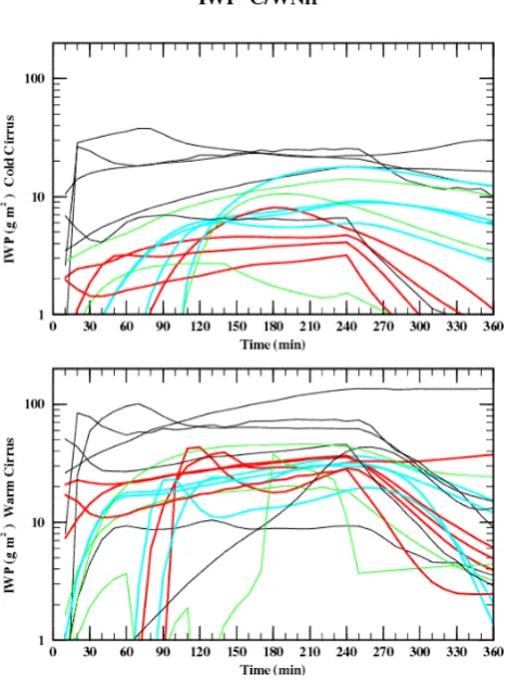
Fig. 4: Time series of vertically-integrated ice water path (g m-2) from cirrus cloud simulations by models participating in the GCSS WG2 ICMC Project. These baseline simulations correspond to nighttime (infrared radiation only) “warm” cirrus (lower panel) and “cold” cirrus (upper panel) cases with cloud tops at about -47°C and -66°C, respectively, subject to continuous cooling representing a 3 cm s-1 uplift over a 4-hour time span followed by a 2-hour dissipation stage. Shown are results from CSMs with “bin” microphysics (cyan), CSMs with bulk microphysics (red), single column models (green), and CSMs with heritage in study of deep convection or boundary layer clouds (thin black). Notice the large range of values produced by these state-of-the-art models after 4 hours of simulation, and that a) bin and bulk CSM results tend to separately cluster, b) SCMs results span the range of CSM results, c) heritage models exhibit larger scatter and d) larger spread is found for the “cold” cirrus case where the dissipation phase is notably different between the bin and bulk models and where observations are especially sparse and uncertain.

Fig. 1. Time series of vertically-integrated ice water path (g m−2) from cirrus models, which participate the ICMCP. These baseline simulations correspond to night-time (infrared radiation only). The upper panel is for the “cold” (about−66◦C) cirrus case and the bot-tom one is for the “warm” (about−47◦C) cirrus case. A 3 cm s−1 uplift is continuously applied over a 4 h time period and then there is a 2-h dissipation time. The colour cyan represents CSMs with bin microphysics, red represents CSMs with bulk microphysics, green represents single column models and the thin black represents CSMs with heritage in the study of deep convection or boundary layer clouds. This figure illustrates the wide range in cirrus model predictions for an idealised case (figure is taken from Starr et al., 2000).

deep convective cloud systems and polar clouds. This has been more recently extended to include other case devel-opments such as Pacific Cross-section Intercomparison, etc. The cirrus working group (WG2) in the past has initiated one previous project focusing on high resolution cloud model inter-comparison. It was denoted the Idealised Cirrus Model Comparison Project (ICMCP) and had 16 models involved in the comparison ranging from cloud scale models (CSMs) to single column models (SCMs) (both GCM SCMs as well as highly detailed 1-D models).

The results of the first inter-comparison (ICMCP) were a surprise to the cirrus community. It showed that the com-munity’s numerical models of cirrus showed significantly

larger disagreement than expected concerning such funda-mental quantities as ice water path (IWP) for even idealised cases. The results appeared only in a conference paper (Starr et al., 2000). Figure 1 is taken from that paper and illustrates the range in results of as much as two orders of magnitude in IWP. There was some separate grouping noted between bin and bulk models, however, the range was large for all cate-gories. The results from SCMs span the whole range of CSM results and models not originally developed for cirrus exhibit larger scatter and generally there was larger scatter for all model categories for the cold case.

In addition to the ICMCP inter-comparison, there was also a Cirrus Parcel Model Comparison Project (CPMCP) (Lin et al., 2002) which was a follow-on project as part of the GCSS WG2. The main aim of their study was to compare the microphysics specification of different cirrus models under idealised conditions. For complete details, refer to Lin et al. (2002).

Although well instrumented sites such as ARM provide significant amounts of data for modelling studies, develop-ing a high-resolution modelldevelop-ing case based in observations is somewhat rare in the literature. Several studies have based their modelling studies on observations such as Brown and Heymsfield (2001) used TOGA-COARE data, Benedetti and Stephens (2001) used ARM data, Cheng et al. (2001) used FIREII data, Marsham and Dobbie (2005) and Marsham et al. (2006) used Chilbolton data, Solch and Karcher (2011) used ARM data, and Yang et al. (2011) used EMERALD1 data; however, these studies are only loosely based on obser-vations and often the large-scale forcing of the cloud layer, which is so important for cloud development (see Lin et al. 2002) is either not available or very approximate.

Comparisons to observations have improved in recent years in that efforts have been made to simulate the remote sensing of radar and radiometers within the models for ease of comparison when evaluating timeseries (Marsham and Dobbie, 2005; Marsham et al., 2006), as well as making use of more and more observations such as modelling returns of Doppler fall velocities (Marsham et al., 2006). Important ad-vances have been made by observationalists since the last inter-comparison in using a synergy of more than one in-strument to improve retrievals (Deng and Mace, 2006; De-lanoe and Hogan, 2008). In this work we utilise remote sens-ing to determine ice content, ice number and fall velocities. This offers great opportunities to test models since models can be easily tuned to a single observation of, say, ice water content (IWC) or ice number concentration (INC); however, observations of three or more variables affords a much bet-ter opportunity to highlight models performing well and also highlight potential deficiencies. We note that one case study is not a definitive assessment of the cirrus models, but offers a good basis to begin with and build upon.

It is important for the cirrus research community to assess current cirrus models and schemes against rigorous observa-tions to determine if cirrus modelling has improved from the

(3)

H. Yang et al.: GCSS WG2 – Case Study 831

developments over the last decade and also use the results to gauge which models are performing well and identify ar-eas for improvement. This is the first cirrus study that in-cludes rigorous comparisons to observations with the added benefit of an inter-comparison framework. This paper begins with describing the observed case of 9 March 2000 at the ARM SGP site and then proceeds to detail how the modelling case was established. This case was issued to the GCSS cir-rus working group members to participate in the modelling inter-comparison; the results of which will be presented in a follow-on paper.

2 ARM SGP IOP 9 March 2000 observations used in the case development

The main aim of the current GCSS cirrus inter-comparison was to compare the model results to observations in order to evaluate model performance. As mentioned, the last inter-comparison showed strong model-to-model variation for re-sults such as IWP with time for even such an idealised case. It is imperative that the cirrus community evaluate their mod-els with observations in as rigorous a way as possible and through multiple comparisons. This case, presented in this work, forms the first step in that process.

The 9 March 2000 case was selected because it was a well-observed case. During the intensive observing period (IOP) at the SGP ARM site in March 2000, cirrus formed just up-wind from the site on the 9th and advected directly over the Central Facility (CF) site. The ARM sites have the most ex-tensive set of routine measurements in the world and this is enhanced with aircraft and supplemental measurements during IOP periods. In addition to the extensive observa-tions taking place, analysis of some key results from the 9th were readily available for the inter-comparison. This in-cluded remote-sensing retrieval of cloud properties, analysis of aircraft observations and objective analysis (Zhang et al., 2000). Unfortunately, aerosol properties were not available at the cloud layer altitude during the cloud evolution relevant for our case development.

2.1 Meteorology and profiles

The region of cirrus that eventually was observed at the CF was first noted as a jet stream maximum in a southwesterly flow that passed over the mountain ranges of central New Mexico. The cirrus thickened as the disturbance approached central Oklahoma and the cloud features appeared to organ-ise into longitudinal bands. Satellite imagery suggested ac-tive development of individual features within these bands as the system passed over the CF. The character of the cir-rus in the satellite plots as well as the large scale atmo-spheric flow suggests that the cloud may be forced by gravity waves from the neighbouring mountains. The objective anal-ysis predicted a weak lifting, whereas the RUC model

indi-Yang et al.: GCSS WG2 - Case Study 3

IWP with time for even such an idealised case. It is impera-tive that the cirrus community evaluate their models with ob-servations in as rigorous a way as possible and through mul-tiple comparisons. This case presented in this work forms the first step in that process.

The March 9th _{2000 case was selected because it was a}

well observed case. During the intensive observing period (IOP) at the SGP ARM site in March 2000, cirrus formed just upwind from the site on the 9thand advected directly over the Central Facility (CF) site. The ARM sites have the most extensive set of routine measurement in the world and this is enhanced with aircraft and supplemental measurements dur-ing IOP periods. In addition to the extensive observations taking place, analysis of some key results from the 9thwere readily available for the inter-comparison. This included re-mote sensing retrieval of cloud properties, analysis of aircraft observations, and objective analysis (Zhang et al., 2000). Un-fortunately, aerosol properties were not available at the cloud layer altitude during the cloud evolution relevant for our case development.

2.1 Meteorology and profiles

The region of cirrus that eventually was observed at the CF was first noted as a jet stream maximum in a southwesterly flow that passed over the mountain ranges of central New Mexico. The cirrus thickened as the disturbance approached central Oklahoma and the cloud features appeared to orga-nize into longitudinal bands. Satellite imagery suggested ac-tive development of individual features within these bands as the system passed over the CF. The character of the cirrus in the satellite plots as well as the large scale atmospheric flow suggests that the cloud may be forced by gravity waves from the neighboring mountains. The objective analysis predicted a weak lifting, whereas the RUC model indicated little to no ascent. This is explored further in the large scale forcing sec-tion below.

The radiosondes were released simultaneously at five lo-cations at three hour intervals during 9th_{March including at}

the CF site and four sites surrounding the CF. These were used to construct the profiles, such as temperature, pressure, horizontal wind profiles, used in the case. The profiles in-dicated a temperature inversion near cloud top and a water vapour peak at 8-9km, where the cloud is observed, as shown in Figure 2.

2.2 Remote sensing

Visible satellite images were analysed from both GOES 8 and 10 for the time period from 00:30 UTC to 23:30 UTC on March 9th_{, 2000. In Figure 3, the blue indicator (with the}

time of 14:00 UTC inside) points to the ARM SGP CF site and the white arrow indicates the location where the cirrus cloud system was first observed to form upwind and south west of the CF. The cloud system is observed to brighten

Fig. 2. Tephi-graph for the March 9th2000 case study. The me-teorological soundings are taken from radiosonde ascents and indi-cate the high water vapour around the 500mb level where the cloud forms.

Institute for Climate and Atmospheric Science (ICAS)

14.00

Fig. 3. GOES10 satellite plot at 14:00 UTC on the 9thof March 2000. The white arrow indicates approximately where the cirrus forms upwind and the ARM Central Facility is denoted by the blue indicator.

and become more extensive in subsequent visible imagery as it advects from the location of formation to the ARM SGP site. The cloud is observed by the MMCR at the CF ap-proximately 210 minutes after the time of formation, at 17:30 UTC.

The remote sensing of the cirrus cloud properties such as

Fig. 2. Tephi-graph for the 9 March 2000 case study. The meteo-rological soundings are taken from radiosonde ascents and indicate the high water vapour between 300 mb and 350 mb level where the cloud forms.

Yang et al.: GCSS WG2 - Case Study 3

IWP with time for even such an idealised case. It is impera-tive that the cirrus community evaluate their models with ob-servations in as rigorous a way as possible and through mul-tiple comparisons. This case presented in this work forms the first step in that process.

The March 9th _{2000 case was selected because it was a}

well observed case. During the intensive observing period (IOP) at the SGP ARM site in March 2000, cirrus formed just upwind from the site on the 9th and advected directly over the Central Facility (CF) site. The ARM sites have the most extensive set of routine measurement in the world and this is enhanced with aircraft and supplemental measurements dur-ing IOP periods. In addition to the extensive observations taking place, analysis of some key results from the 9thwere readily available for the inter-comparison. This included re-mote sensing retrieval of cloud properties, analysis of aircraft observations, and objective analysis (Zhang et al., 2000). Un-fortunately, aerosol properties were not available at the cloud layer altitude during the cloud evolution relevant for our case development.

2.1 Meteorology and profiles

The region of cirrus that eventually was observed at the CF was first noted as a jet stream maximum in a southwesterly flow that passed over the mountain ranges of central New Mexico. The cirrus thickened as the disturbance approached central Oklahoma and the cloud features appeared to orga-nize into longitudinal bands. Satellite imagery suggested ac-tive development of individual features within these bands as the system passed over the CF. The character of the cirrus in the satellite plots as well as the large scale atmospheric flow suggests that the cloud may be forced by gravity waves from the neighboring mountains. The objective analysis predicted a weak lifting, whereas the RUC model indicated little to no ascent. This is explored further in the large scale forcing sec-tion below.

The radiosondes were released simultaneously at five lo-cations at three hour intervals during 9thMarch including at the CF site and four sites surrounding the CF. These were used to construct the profiles, such as temperature, pressure, horizontal wind profiles, used in the case. The profiles in-dicated a temperature inversion near cloud top and a water vapour peak at 8-9km, where the cloud is observed, as shown in Figure 2.

2.2 Remote sensing

Visible satellite images were analysed from both GOES 8 and 10 for the time period from 00:30 UTC to 23:30 UTC on March 9th_{, 2000. In Figure 3, the blue indicator (with the}

time of 14:00 UTC inside) points to the ARM SGP CF site and the white arrow indicates the location where the cirrus cloud system was first observed to form upwind and south west of the CF. The cloud system is observed to brighten

Fig. 2. Tephi-graph for the March 9th2000 case study. The me-teorological soundings are taken from radiosonde ascents and indi-cate the high water vapour around the 500mb level where the cloud forms.

Institute for Climate and Atmospheric Science (ICAS)

14.00

Fig. 3. GOES10 satellite plot at 14:00 UTC on the 9th_{of March}

2000. The white arrow indicates approximately where the cirrus forms upwind and the ARM Central Facility is denoted by the blue indicator.

and become more extensive in subsequent visible imagery as it advects from the location of formation to the ARM SGP site. The cloud is observed by the MMCR at the CF ap-proximately 210 minutes after the time of formation, at 17:30 UTC.

The remote sensing of the cirrus cloud properties such as

Fig. 3. GOES10 satellite plot at 14:00 UTC on the 9th of March 2000. The white arrow indicates approximately where the cirrus forms upwind and the ARM Central Facility is denoted by the blue indicator.

cated little to no ascent. This is explored further in the large scale forcing section below.

The radiosondes were released simultaneously at five lo-cations at three hour intervals during 9 March, including the CF site and four sites surrounding the CF. These were used to construct the profiles, such as temperature, pressure,

(4)

horizontal wind profiles used in the case. The profiles in-dicated a temperature inversion near cloud top and a wa-ter vapour peak at 8–9 km, where the cloud is observed, as shown in Fig. 2.

2.2 Remote sensing

Visible satellite images were analysed from both GOES 8 and 10 for the time period from 00:30 UTC to 23:30 UTC on 9 March 2000. In Fig. 3, the blue indicator (with the time of 14:00 UTC inside) points to the ARM SGP CF site and the white arrow indicates the location where the cirrus cloud system was first observed to form upwind and south west of the CF. The cloud system is observed to brighten and become more extensive in subsequent visible imagery as it advects from the location of formation to the ARM SGP site. The cloud is observed by the MMCR at the CF approximately 210 min (at 17:30 UTC) after the time of formation.

The remote sensing of the cirrus cloud properties such as IWC, INC, and ice particle fall speeds is crucial to the case study. An important reason for choosing this case study was that these cloud properties were already analysed (by G. G. Mace, Utah) and available for this study (Mace, 1998). The retrieval is based on algorithms using radar reflectiv-ity and downwelling infrared radiances to evaluate the cir-rus cloud microphysical properties (Matrosov et al., 1992; Matrosov et al., 1994). The layer-averaged properties of op-tically thin cirrus is applied, which is calculated by using the observational platforms at the ARM sites. The layer-mean particle size distribution (PSD) (Mace, 1998) is the main as-sumption in this method, in which a modified gamma func-tion (Dowling and Radke, 1990) is used. The PSD equafunc-tion is

N (D)=Nxexp(α)

D Dx

exp

−Dα

Dx

(1) whereDxis the modal diameter,Nxis the number of parti-cles per unit volume, per unit length at the functional maxi-mum andαis the order of the distribution, which is suggested

≤2 for cirrus (Dowling and Radke, 1990).

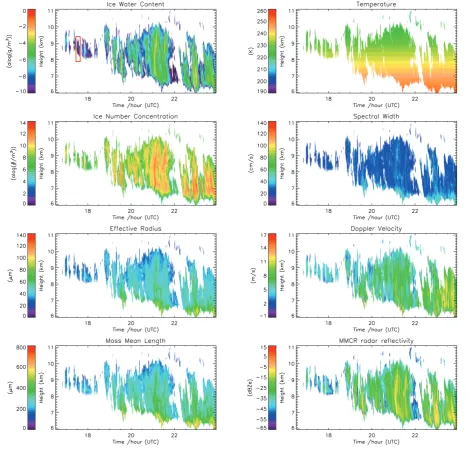
Shown in Fig. 4 is the retrieved IWC, INC, effective size and mean mass length, etc., as functions of time. The errors in IWC and median particle size are of the order of 60 % and 40 %, respectively (see Mace et al., 2002). The case development focuses on cloud that first forms upwind and then advects over the SGP CF site and is remotely sensed at 17:30 UTC (shown in Fig. 4). It is evident in the retrievals that the cloud increases in IWC as it advects over the SGP site and thickens in vertical extent.

2.3 Aircraft turbulence observations

University of North Dakota’s Cessna Citation aircraft under-took 12 flights as part of the IOP, in March 2000, includ-ing flight penetrations at various altitudes through the cirrus

cloud on the 9th. This flight started at 18:32 h which is af-ter our first cloud appearance at the CF, so it is not an exact match with our comparison time. But it appears reasonable to assume that the turbulence observed by the aircraft measure-ments is representative for the cloud at an earlier stage. The mean wind and wind turbulence were measured by five-hole-probe (Validyne P40d) in combination with INS/GPS (Litton LTN-76). The sampling rate is 25 Hz and the uncertainty for turbulent fluctuations is about 0.05 m s−1. The true airspeed (to estimate length scales) was mostly about 120 m s−1. The power spectra of the vertical wind velocity,w, along flight legs at different altitudes, as shown in Fig. 5, indicates a scale separation at about 320 m length scale (roughly 0.4 Hz). The scale of large eddies is about 200 m (roughly 0.6 Hz) and the inertial sub-range starts showing up at a scale of about 100 m (roughly 1.2 Hz). The power spectra indicates that the turbulent kinetic energy is considerably higher in the cloud top region compared to the base. Based on the scale lengths deduced from the turbulence observations, we decided that 100 m grid resolution in the cloud layer for the LEM simula-tions would be appropriate.

2.4 Large scale forcing

The large scale forcing is critical for obtaining a good mod-elling case study, as it has such an important influence on the formation and magnitude of the cloud. For the March 2000 IOP at the ARM SGP site, objective analysis has been per-formed to assess the large-scale forcing, so we begin with this.

2.4.1 Objective analysis

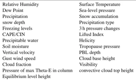
Objective analysis for the March 2000 IOP and results are summarised in Zhang et al. (2000). We summarise key points from the paper below; for specific details of the method please refer to Zhang et al. (2000). The objective analysis used is a constrained variational analysis method (CVAM) which was originally developed by Zhang and Lin (1997) with a second improvement in 2000. CVAM was developed for deriving large-scale vertical velocity and advective ten-dencies from sounding measurements and works with the raw data from even a small number of stations. It can refine these atmospheric state variables as well as give uncertain-ties in the original data. The CVAM approach requires large-scale variables (u, v, T, q), surface measurements including surface sensible and latent heat fluxes, precip, surface pres-sure, surface winds, surface temperature, surface broadband net radiative flux and column total cloud water.

The observed data for these variables are used in this analysis which includes conservation of column-integrated mass, water, energy and momentum (Zhang et al., 2000). The data used in the CVAM approach are variables col-lected from the ARM balloon-borne sounding and National Oceanic and Atmospheric Administration (NOAA) wind

(5)

Fig. 4. Remotely sensed quantities as a function of height and time. The quantities include total IWC, total INC, effective radius, mean mass length, temperature, spectral width, Doppler velocity and reflectivity. Units indicated in the plots. The plots based on retrievals at the ARM SGP CF for 9 March 2000. The inter-comparison is based on the cloud when it arrives at the CF at approximately 17:30 UTC and indicated on the left side of each plot. The red box in the top left panel indicates the comparison period for modelling and retrievals.

profile measurements. Figure 6a shows there is one balloon launch site located at the CF of the ARM site and another four launch sites around the CF at the boundary facilities.

During the IOP 2000, sounding balloons were launched every three hours to measure the variables such as tempera-ture, pressure, water vapour mixing ratio and wind profiles. In addition, the objective analysis makes use of seventeen NOAA wind profilers surrounding the SGP site. Seven of which are near the CF and five vertical profilers exactly over-lap with the sounding stations, as shown in Fig. 6b. The seven sites constitute the domain of the objective analysis. One

ad-ditional grid point is added in each boundary site to improve the linear assumption Fig. 6c. The Cressman scheme (Cress-man, 1959) is used for the upper air measurement, making use of the general weighting function according to:

wik=w(xi, xk)=

(

1

N

L2−(xi−xk)2

L2₊_(x

i−xk)2, dik< L

0, otherwise (2)

where thewik is the weighting coefficient,k indicates the

observational points and i is the analysis grid point, xi is

any variable in three or four dimensions at the grid point,

(6)

6 Yang et al.: GCSS WG2 - Case Study

Fig. 5. Power spectrum of vertical velocity obtained from aircraft observations. Pertinent scales are: separation length scale is 320 m ∼0.4 Hz, large eddies occur at roughly 200 meters∼0.6 Hz, and the inertial sub-range starts showing up at a scale of about 100 m∼ 1.2 Hz.

Fig. 6. Latitude and longitude locations of the a) radiosonde launches, b) the radiosonde launch sites and profiles, c) additional profilers and grid, and d) the RUC model grid. (The plots are taken from Zhang et al., 2000)

where thewikis the weighting coefficient,kindicates the

xk(k= 1,2,...,K), observation stations,Niis the number of

measurements within distanceL, anddikis the distance

be-tween the measurements and grid point.

Fig. 7.Large scale vertical velocity from OA at 3pm 9th2000.

The output from NOAA RUC is used in Eq. 3 as the value for the background function,fb(shown in Figure 6d). The

general form used to evaluate the objective analysis variables at each grid-point is given by:

fa(xi) =fb(xi) + k=K

X

k=1

wik[fo(xk)−fb(xk)] (3)

For further details refer to Zhang et al (2000). There is also a comprehensive set of surface measurements, as indi-cated in Table 1, around the SGP site and measurements from satellites such as GOES.

There are three frequently used area-based data analysis approaches for objective analysis including the analytical fit-ting method, the line integral method and the regular grid method. The ARM SGP objective analysis method uses a hybrid approach of the regular-grid and line integral meth-ods and a variational constraining procedure (Zhang and Lin, 1997). The large scale variables diagnosed from the objec-tive analysis are listed in Table 2.

From the objective analysis, we illustrate in Figure 7 the large scale vertical motion at 1500 UTC which is at the time the cirrus has already formed and is advecting toward the CF at SGP. The vertical velocity at 8-9km height is approxi-mately 0.01 m/s.

2.4.2 RUC model results

The regional (large-scale for our 10km domain high reso-lution simulations) scale updraft is obtained using the pro-files from the objective analysis with the RUC operational atmospheric prediction system. RUC is an analysis system and numerical forecast model which had its origins in the Mesoscale Analyses and Prediction System (MAPS) which

Fig. 5. Power spectrum of vertical velocity obtained from air-craft observations. Pertinent scales are: separation length scale is 320 m∼0.4 Hz, large eddies occur at roughly 200 m∼0.6 Hz, and the inertial sub-range starts showing up at a scale of about 100 m∼1.2 Hz.

6 Yang et al.: GCSS WG2 - Case Study

Fig. 5. Power spectrum of vertical velocity obtained from aircraft observations. Pertinent scales are: separation length scale is 320 m

∼0.4 Hz, large eddies occur at roughly 200 meters∼0.6 Hz, and the inertial sub-range starts showing up at a scale of about 100 m∼

1.2 Hz.

where thewikis the weighting coefficient,kindicates the

xk(k= 1,2,...,K), observation stations,Ni is the number of

measurements within distanceL, anddik is the distance

The output from NOAA RUC is used in Eq. 3 as the value for the background function, fb (shown in Figure 6d). The

fa(xi) =fb(xi) + k=K

X

k=1

For further details refer to Zhang et al (2000). There is also a comprehensive set of surface measurements, as indi-cated in Table 1, around the SGP site and measurements from satellites such as GOES.

There are three frequently used area-based data analysis approaches for objective analysis including the analytical fit-ting method, the line integral method and the regular grid method. The ARM SGP objective analysis method uses a hybrid approach of the regular-grid and line integral meth-ods and a variational constraining procedure (Zhang and Lin, 1997). The large scale variables diagnosed from the objec-tive analysis are listed in Table 2.

From the objective analysis, we illustrate in Figure 7 the large scale vertical motion at 1500 UTC which is at the time the cirrus has already formed and is advecting toward the CF at SGP. The vertical velocity at 8-9km height is approxi-mately 0.01 m/s.

2.4.2 RUC model results

The regional (large-scale for our 10km domain high reso-lution simulations) scale updraft is obtained using the pro-files from the objective analysis with the RUC operational atmospheric prediction system. RUC is an analysis system and numerical forecast model which had its origins in the Mesoscale Analyses and Prediction System (MAPS) which

Fig. 6. Latitude and longitude locations of the (a) radiosonde launches, (b) the radiosonde launch sites and profiles, (c) additional profilers and grid, and (d) the RUC model grid. (The plots are taken from Zhang et al., 2000).

xk(k=1,2, ..., K), observation stations,Ni is the number of

measurements within distanceL, anddik is the distance

The output from NOAA RUC is used in Eq. (3) as the value for the background function,fb(shown in Fig. 6d). The

6 Yang et al.: GCSS WG2 - Case Study

Fig. 5. Power spectrum of vertical velocity obtained from aircraft observations. Pertinent scales are: separation length scale is 320 m

∼0.4 Hz, large eddies occur at roughly 200 meters∼0.6 Hz, and the inertial sub-range starts showing up at a scale of about 100 m∼

1.2 Hz.

where the

w

ik

is the weighting coefficient,

k

indicates the

observational points and

i

is the analysis grid point,

x

i

is

any variable in three or four dimensions at the grid point,

x

k

(

k

= 1

,

2 ,...,K

)

, observation stations,

N

i

is the number of

measurements within distance

L

, and

d

ik

is the distance

be-tween the measurements and grid point.

The output from NOAA RUC is used in Eq. 3 as the value

for the background function,

f

b

(shown in Figure 6d). The

general form used to evaluate the objective analysis variables

at each grid-point is given by:

f

a

(

x

i

) =

f

b

(

x

i

) +

k=K

X

k=1

w

ik

[

f

o

(

x

k

)

−

f

b

(

x

k

)]

(3)

For further details refer to Zhang et al (2000). There is

also a comprehensive set of surface measurements, as

indi-cated in Table 1, around the SGP site and measurements from

satellites such as GOES.

There are three frequently used area-based data analysis

approaches for objective analysis including the analytical

fit-ting method, the line integral method and the regular grid

method. The ARM SGP objective analysis method uses a

hybrid approach of the regular-grid and line integral

meth-ods and a variational constraining procedure (Zhang and Lin,

1997). The large scale variables diagnosed from the

objec-tive analysis are listed in Table 2.

From the objective analysis, we illustrate in Figure 7 the

large scale vertical motion at 1500 UTC which is at the time

the cirrus has already formed and is advecting toward the

CF at SGP. The vertical velocity at 8-9km height is

approxi-mately 0.01 m/s.

2.4.2 RUC model results

The regional (large-scale for our 10km domain high

reso-lution simulations) scale updraft is obtained using the

pro-files from the objective analysis with the RUC operational

atmospheric prediction system. RUC is an analysis system

and numerical forecast model which had its origins in the

Mesoscale Analyses and Prediction System (MAPS) which

Fig. 7. Large scale vertical velocity from OA at 03:00 pm 9 March 2000.

fa(xi)=fb(xi)+ k=K

X

k=1

For further details refer to Zhang et al. (2000). There is also a comprehensive set of surface measurements, as indi-cated in Table 1, around the SGP site and measurements from satellites such as GOES.

There are three frequently used area-based data analysis approaches for objective analysis including the analytical fit-ting method, the line integral method and the regular grid method. The ARM SGP objective analysis method uses a hybrid approach of the regular-grid and line integral meth-ods and a variational constraining procedure (Zhang and Lin, 1997). The large scale variables diagnosed from the objective analysis are listed in Table 2.

From the objective analysis, we illustrate in Fig. 7 the large scale vertical motion at 15:00 UTC which is at the time the cirrus has already formed and is advecting toward the CF at SGP. The vertical velocity at 8–9 km height is approximately 0.01 m s−1.

2.4.2 RUC model results

To complement the OA, we also investigated the large scale forcing predicted by the RUC model. The regional (large-scale for our 10 km domain high resolution simulations) scale updraft is obtained using the profiles from the objec-tive analysis with the RUC operational atmospheric predic-tion system. RUC is an analysis system and numerical fore-cast model which had its origins in the Mesoscale Analyses

(7)

Table 1. The surface measurement used by the objective analysis at the ARM SGP site at Oklahoma USA, used for the objective analysis during the 9 March 2000 campaign and the variables measured by each instrument.

Platform Name Variables Measured

Surface Meteorological Observation Stations(SMOS) surface pressure, surface winds, temperature, humidity

Energy Budget Bowen Ratio (EBBR) Stations surface latent and sensible heat fluxes, surface broadband net radiative flux Eddy Correlation Flux Measurement System (ECOR) surface vertical fluxes of momentum, sensible heat flux, latent heat flux Oklahoma and Kansas mesonet stations (OKM and KAM) surface precipitation, pressure, winds, temperature

Microwave Radiometer (MWR) stations column precipitable water, total cloud liquid water

GOES satellite clouds and broadband radiative fluxes

Table 2. The diagnosed variables output by the Objective Analysis

Relative Humidity Surface Temperature Dew Point Sea-level pressure Precipitation Snow accumulation snow depth Precipitation type Freezing levels 3 h pressure changes CAPE/CIN Lifted Index Precipitable water Helicity

Soil moisture Tropopause pressure Vertical velocity PBL depth Gust wind speed Cloud base height Cloud fraction Visibility

Pressure of max Theta-E in column convective cloud top height Equilibrium level height

and Prediction System (MAPS) which was developed at the Forecast Systems Laboratory (FSL) in 1988. The first RUC model with a 3 h data assimilation cycle, 60 km resolution, and vertical 25 levels was established at the National Cen-ter for Environmental prediction (NCEP) in 1994. In 1998, this was followed by the RUC-2 model which had a 1 h data assimilation cycle, 40 km resolution and 40 levels. RUC-20 (20 km resolution, 50 levels) and RUC13 (13 km resolution, 50 levels) were developed in 2002 and 2005 separately. Pro-viding short range weather forecasts is the primary use of RUC model and evaluation of other models. The diagnostic variables derived from RUC model is listed in Table 2.

The RUC model, being initialised with updated data every hour, is a great strength as well as the fact that all the data are on isentropic vertical levels. The horizontal resolution, how-ever, is a weakness for this case as it is still insufficient to describe local topographical circulations for this high resolu-tion case.

For 9 March, the RUC model indicates little to no as-cent rate (approximately zero and certainly bounded by 0.0016 m s−1) in the region in which the cirrus cloud is formed. So in summary, the objective analysis indicates a weak ascent whereas the RUC model indicates essentially no ascent. Since the objective analysis is making use of ob-served local data to where the cloud is obob-served and this data may contain signatures in the data of local forcings, we seek

to explain the difference in forcings between the objective analysis results and the RUC model prediction.

Given that the direction of the mean atmospheric flow at cloud level is over the Rocky Mountains on the 9 March and the SGP CF is on the lee side of the mountains, the vertical motion could be explained by gravity waves. This could ex-plain why the objective analysis suggested a larger vertical velocity than the RUC model. In order to evaluate the po-tential of gravity waves to influence the cirrus formation, we have performed gravity wave simulations for the whole of the USA for 9 March 2000 using the model 3DVOM described in the next section.

2.4.3 Gravity wave analysis using 3DVOM

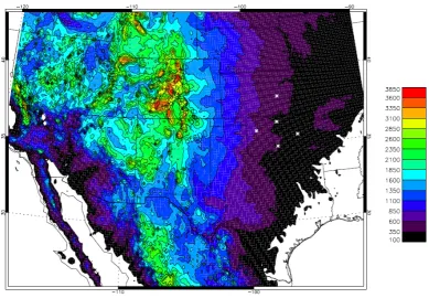
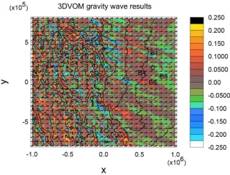
As shown in Fig. 8, the most prominent topological feature in this map of the USA is the Rocky Mountains (RM). The RM extend for more than 3000 miles in length and cover approx-imately 300 000 square miles and are positioned to the west of the SGP ARM site. With a south-west atmospheric advec-tion, the influence of gravity waves on the cirrus formation on the lee side of the mountains is highly likely.

In this study, we make use of the 3DVOM model called 3-D velocities over mountains which is a finite-difference numerical model designed for high-resolution simulations of lee waves generated by flow over complex terrain.

The model is based on a set of time-dependent, simpli-fied, quasi-linear equations of motion for a dry atmosphere (see Vosper and Worthington 2002; 2003 for details), typi-cally run with European Centre for Medium Range Weather Forecasting (ECMWF) winds. The model was run at a 1 km resolution for the entire USA, initialised in this case with NCEP winds and the topology specified from the data that went into making Fig. 8.

The resulting map of gravity wave vertical motion deter-mined by 3DVOM at the cloud level is shown in Fig. 9. It shows clearly that gravity waves are predicted to cause as-cending motion in the region where the cloud forms (roughly 300 km upwind) and during much of its advection toward the SGP CF site. Consequently, to obtain the vertical forcing for the high resolution cloud resolving simulation, we extracted

(8)

8 Yang et al.: GCSS WG2 - Case Study

Fig. 8. Topology of the USA (m). This is used to initialise the surface heights for the gravity wave simulations in the 3DVOM model. The white dots indicate the ARM SGP Central and Boundary Facilities (data from Global Land One-km Base Elevation (GLOBE) project).

numerical model designed for high-resolution simulations of

lee waves generated by flow over complex terrain.

The model is based on a set of time-dependent, simplified,

quasi-linear equations of motion for a dry atmosphere (see

Vosper and Worthington 2002; 2003 for details), typically

run with European Centre for Medium Range Weather

Fore-casting (ECMWF) winds. The model was run at 1km

reso-lution for the entire USA, initialised in this case with NCEP

winds and the topology specified from the data that went into

making Figure 8.

The resulting map of gravity wave vertical motion

deter-mined by 3DVOM at the cloud level is shown in Figure 9.

It shows clearly that gravity waves are predicted to cause

as-cending motion in the region where the cloud forms (roughly

300 km upwind) and during much of its advection toward the

SGP CF site. Consequently, to obtain the vertical forcing for

the high resolution cloud resolving simulation, we extracted

the vertical forcing from Figure 9 along the advection path

of the cirrus cloud from formation to the SGP CF. The

grav-ity wave forcing at cirrus cloud level as a function of time is

given in Figure 10.

The plot of vertical velocity forcing as a function of height

and time, shown in Figure 10, indicates gravity waves

su-perimposed with various wavelengths that are undergoing

an ascent (hence cooling) beginning at the location where

the cirrus is observed to first form. This agrees very well

with where the cloud forms from satellite observation and

the gravity wave forcing intensifies as the cloud advects

to-Fig. 9. Gravity wave plot at the cirrus level for March 9th 2000. Colour codes indicate ascent rate (positive) or descent (negative) in m/s. These results are derived from the output of 3DVOM model runs.

ward the SGP site, in agreement with the satellite

observa-tion. In the final stages of when the cloud is advecting over

the SGP site, the gravity wave undergoes descent. So the

modelled gravity wave forcing provides ascent or cooling to

the cloud layer that is consistent with maintaining a cirrus

cloud layer as it advects toward the CF site. We also note

Fig. 8. Topology of the USA (m). This is used to initialise the surface heights for the gravity wave simulations in the 3DVOM model. The

white dots indicate the ARM SGP Central and Boundary Facilities (data from Global Land One-km Base Elevation (GLOBE) project).

the vertical forcing from Fig. 9 along the advection path of the cirrus cloud from formation to the SGP CF. The grav-ity wave forcing at cirrus cloud level as a function of time is given in Fig. 10.

The plot of vertical velocity forcing as a function of height and time, shown in Fig. 10, indicates gravity waves superim-posed with various wavelengths that are undergoing an as-cent (hence cooling) beginning at the location where the cir-rus is observed to first form. This agrees very well with where the cloud forms from satellite observation and the gravity wave forcing intensifies as the cloud advects toward the SGP site, in agreement with the satellite observation. In the fi-nal stages of when the cloud is advecting over the SGP site, the gravity wave undergoes descent. So the modelled gravity wave forcing provides ascent or cooling to the cloud layer that is consistent with maintaining a cirrus cloud layer as it advects toward the CF site. We also note that the mean ver-tical velocity from the gravity wave simulation agrees well with the vertical velocity from the objective analysis.

3 Model setup and first results

We now describe how the observations were used to set up the modelling study and first results are illustrated just for the UK Met Office large eddy simulation model (LEM) to test

if the case is appropriate for an inter-comparison. We begin with a brief description of the LEM model.

3.1 UK LEM Model

To establish the modelling case based on the 9 March ARM SGP observations, we used the UK Met Office Large Eddy Model (LEM) v2.3 (Mace, 1998; Gray et al., 2001). The UK Met Office LEM performs numerical integrations using basic equations for momentum, thermodynamics and continuity. The model is non-hydrostatic and uses the deep anelastic ap-proximation (quasi-Boussinesq) which allows for small pres-sure and density variations from the reference hydrostatic state. Periodic boundary conditions are used at the horizontal edges of the domain and rigid lid conditions are used at the surface and top of model boundaries. The model has been used for several studies of cirrus (Dobbie and Jonas, 2001; Marsham and Dobbie, 2005; Marsham et al., 2006; Yang et al., 2011). The version we use has a fully integrated Fu-Liou radiation scheme to address the radiative properties and heat-ing rates of the cloud. Details of the radiation scheme are pro-vided below and in papers such as Dobbie and Jonas (2001), Marsham and Dobbie (2005) and Marsham et al. (2006). We provide a brief description here. The radiation model used is based on Fu and Liou (1992, 1993) with an ice radia-tion package (Fu, 1996; Fu et al., 1998) and is coupled with the LEM and used to assess cirrus radiative properties, as

(9)

8 Yang et al.: GCSS WG2 - Case Study

Fig. 8.

Topology of the USA (m). This is used to initialise the surface heights for the gravity wave simulations in the 3DVOM model. The

white dots indicate the ARM SGP Central and Boundary Facilities (data from Global Land One-km Base Elevation (GLOBE) project).

numerical model designed for high-resolution simulations of

lee waves generated by flow over complex terrain.

The model is based on a set of time-dependent, simplified,

quasi-linear equations of motion for a dry atmosphere (see

Vosper and Worthington 2002; 2003 for details), typically

run with European Centre for Medium Range Weather

Fore-casting (ECMWF) winds. The model was run at 1km

reso-lution for the entire USA, initialised in this case with NCEP

winds and the topology specified from the data that went into

making Figure 8.

The resulting map of gravity wave vertical motion

deter-mined by 3DVOM at the cloud level is shown in Figure 9.

It shows clearly that gravity waves are predicted to cause

as-cending motion in the region where the cloud forms (roughly

300 km upwind) and during much of its advection toward the

SGP CF site. Consequently, to obtain the vertical forcing for

the high resolution cloud resolving simulation, we extracted

the vertical forcing from Figure 9 along the advection path

of the cirrus cloud from formation to the SGP CF. The

grav-ity wave forcing at cirrus cloud level as a function of time is

given in Figure 10.

The plot of vertical velocity forcing as a function of height

and time, shown in Figure 10, indicates gravity waves

su-perimposed with various wavelengths that are undergoing

an ascent (hence cooling) beginning at the location where

the cirrus is observed to first form. This agrees very well

with where the cloud forms from satellite observation and

the gravity wave forcing intensifies as the cloud advects

to-Fig. 9.

Gravity wave plot at the cirrus level for March 9

th

2000.

Colour codes indicate ascent rate (positive) or descent (negative) in

m/s. These results are derived from the output of 3DVOM model

runs.

ward the SGP site, in agreement with the satellite

observa-tion. In the final stages of when the cloud is advecting over

the SGP site, the gravity wave undergoes descent. So the

modelled gravity wave forcing provides ascent or cooling to

the cloud layer that is consistent with maintaining a cirrus

cloud layer as it advects toward the CF site. We also note

Fig. 9. Gravity wave plot at the cirrus level for 9 March 2000. Colour codes indicate ascent rate (positive) or descent (negative) in m s−1. These results are derived from the output of 3DVOM model runs.

Yang et al.: GCSS WG2 - Case Study 9

Fig. 10. Modelled gravity wave forcing (m/s) versus time (hours). This is the modelled gravity wave forcing that the cloud experiences as it advects from where it first formed to when it arrives at the ARM SGP CF, where it is observed by the MMCR radar.

that the mean vertical velocity from the gravity wave simula-tion agrees well with the vertical velocity from the objective analysis.

3 Model setup and first results

We now describe how the observations were used to set up the modeling study and first results are illustrated just for the UK Met Office large eddy simulation model (LEM) to test if the case is appropriate for an inter-comparison. We begin with a brief description of the LEM model.

3.1 UK LEM Model

To establish the modelling case based on the 9th_{March ARM}

SGP observations, we used the UK Met Office Large Eddy Model (LEM) v2.3 (Mace, 1998; Gray et al., 2001). The UK Met Office LEM performs numerical integrations using basic equations for momentum, thermodynamics, and continuity. The model is non-hydrostatic and uses the deep anelastic ap-proximation (quasi-Boussinesq) which allows for small pres-sure and density variations from the reference hydrostatic state. Periodic boundary conditions are used at the horizontal edges of the domain and rigid lid conditions are used at the surface and top of model boundaries. The model has been used for several studies of cirrus (Dobbie and Jonas, 2001; Marsham and Dobbie, 2005; Marsham et al., 2006; Yang et al., 2011).

The version we use has a fully integrated Fu-Liou radia-tion scheme to address the radiative properties and heating rates of the cloud. Details of the radiation scheme are pro-vided below and in papers such as Dobbie and Jonas (2001), Marsham and Dobbie (2005), and Marsham et al. (2006). We provide a brief description here. The radiation model used is based on Fu and Liou (1992, 1993) with an ice ra-diation package (Fu, 1996; Fu et al., 1998) and is coupled with the LEM and used to assess cirrus radiative

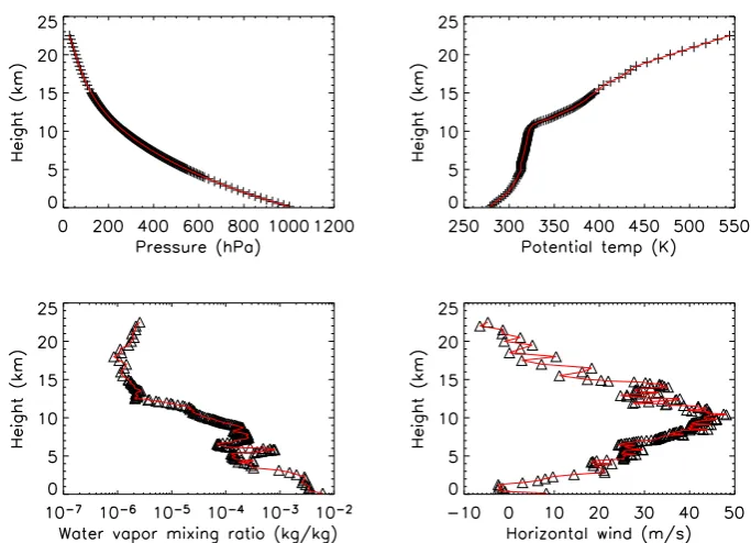
proper-Fig. 11.Initial profiles of pressure, potential temperature, horizon-tal wind, and water vapour mixing ratio at the start location upwind from the CF. The profiles are obtained by taking the observed values at the CF and backtracking them through the effects of the gravity wave to the starting location. This ensures that the profiles will be as observed after the effects of the gravity wave in the modelling.

ties, as was done by Dobbie and Jonas (2001), Marsham and Dobbie (2005), Marsham et al. (2006), and Yang et al. (2011). The radiative transfer equation solution is derived us-ing the discrete ordinates delta four-stream solution approach as discussed in Liou (1986) or papers such as Li and Dobbie (1997).

The Fu-Liouδ-four-stream model is a 1D algorithm that is applied to all columns independently. The Fu-Liou radiation model has six solar and twelve infrared bands. The scheme is linked to the water in the LEM including ice, liquid droplets, rain, graupel, snow, and water vapour. For the case study, the optical properties are specified using the cloud IWC and a value of generalised effective size of 35µm (a similar ap-proach also used in water clouds, see Dobbie and Jonas, 2001), which is in keeping with the observations after con-verting between generalised effective size and effective size and observations more generally (see Fu, 1996). Rayleigh scattering is treated for molecules and gaseous absorption is implemented using a correlated k-distribution method in-cluding gaseous absorption by O3, CO2, CH4, N2O and

H2O. TheCO2,CH4 andN2Oare assumed to have

uni-form mixing ratios throughout the atmosphere with concen-trations of 330, 1.6 and 0.28 ppmv, respectively.

3.2 Model setup for the GCSS inter-comparison

The model domain size was 10 km in the horizontal by 20 km in the vertical. The horizontal resolution was set to 100 m and a variable vertical resolution was used with 100 m resolution for much of the domain (from 5 km to 10 km) and including the cloud layer, with lower resolution above and

Fig. 10. Modelled gravity wave forcing (m s−1) versus time (h). This is the modelled gravity wave forcing that the cloud experiences as it advects from where it first formed to when it arrives at the ARM SGP CF, where it is observed by the MMCR radar.

was done by Dobbie and Jonas (2001), Marsham and Dobbie (2005), Marsham et al. (2006) and Yang et al. (2011). The ra-diative transfer equation solution is derived using the discrete ordinates delta four-stream solution approach as discussed in Liou (1986) or papers such as Li and Dobbie (1997).

The Fu-Liouδ-four-stream model is a 1-D algorithm that is applied to all columns independently. The Fu-Liou radi-ation model has six solar and twelve infrared bands. The scheme is linked to the water in the LEM including ice, liq-uid droplets, rain, graupel, snow and water vapour. For the case study, the optical properties are specified using the cloud

IWC and a value of generalised effective size of 35 µm (a similar approach also used in water clouds, see Dobbie et al., 1999), which is in keeping with the observations after con-verting between generalised effective size and effective size and observations more generally (see Fu, 1996). Rayleigh scattering is treated for molecules and gaseous absorption is implemented using a correlated k-distribution method in-cluding gaseous absorption by O3, CO2, CH4, N2O and H2O. The CO2, CH4and N2O are assumed to have uniform mixing ratios throughout the atmosphere with concentrations of 330, 1.6 and 0.28 ppmv, respectively.

3.2 Model setup for the GCSS inter-comparison The model domain size was 10 km in the horizontal by 20 km in the vertical. The horizontal resolution was set to 100 m and a variable vertical resolution was used with 100 m resolution for much of the domain (from 5 km to 10 km) and includ-ing the cloud layer, with lower resolution above and below this region. The resolution was selected based on the aircraft turbulence analysis presented which indicated it was an ap-propriate scale in which to separate resolved and unresolved motions. The model simulation time was four hours duration. Time zero is associated with 14:00 UTC when the cloud first forms. No cloud is initially specified in the model.

At the first time step of the simulation, random perturba-tions in potential temperature of ±10 % and water vapour mixing ratio of±5 % are imposed between 6 and 10.5 km to

(10)

Fig. 11. Initial profiles of pressure, potential temperature, horizontal wind and water vapour mixing ratio at the start location upwind from the CF. The profiles are obtained by taking the observed values at the CF and backtracking them through the effects of the gravity wave to the starting location. This ensures that the profiles will be as observed after the effects of the gravity wave in the modelling.

establish initial inhomogeneity in the cloud layer (see Mar-sham and Dobbie, 2005).

We impose two forcings on the simulations in the inter-comparison, first a large scale gravity wave forcing updated every 201 s during the simulation. The gravity wave forcing is applied throughout the whole vertical domain for simplic-ity. Second, a Solar and infrared radiative heating profile is applied at every time step and updated every 5 min.

Periodic boundary conditions are used at the horizontal limits of the domain and in the vertical no slip conditions are imposed at the surface and top of the model atmosphere. Heterogeneous and homogeneous nucleation modes are per-mitted in the runs. Horizontal winds are specified from the radiosonde vector-resolved winds into the direction of the ad-vection.

The MMCR based at the SGP CF is the key remote-sensing tool used to obtain the comparison fields for the case and so its location at CF is the point at which the cir-rus cloud is compared quantitatively with the remote sens-ing. The cloud, however, forms approximately 300 km up-wind from the CF. Thus, we have a choice to either spin-up the modelled cloud to agree with the observations at the CF (thereby ignoring the formation and evolution phase) or to model the formation and evolution during advection to the SGP CF and compare with observations at that time.

For this case development, the latter approach was taken, to form the cloud in the model based purely on the forcings acting to create the cloud rather than spin up the model cloud

to artificially “agree” with an observed cloud which has a long history of evolution and is continuously changing as it advects over the observing point at the SGP CF.

So we must recreate the conditions upwind when the cloud formed. We have a few constraints available to do this. From the satellite observations, the cirrus cloud was observed to first form at 14:00 UTC and took about 210 min to advect to the CF, roughly 300 km distance. Also, we know the thermo-dynamic profiles observed at the CF after the cloud advects to the CF. This is after the profiles have undergone forcings during the prior 210 min during the time when the cloud ad-vects from formation location to the CF. Therefore, to obtain the profiles local to where the cloud formed, we apply the forcing in reverse to obtain the initial profiles. This ensures that when the profiles are forced during the 210 min advect-ing to the CF they will then agree with the observed profiles. We know the cloud first forms with the initial upwind pro-files. It was necessary to adjust the initial cloud layer rela-tive humidity to have a slight super-saturation with respect to ice of 10 %. This was equivalent to applying a small tem-perature adjustment of 1–2 K in the cloud layer, which is within observed error, so as to ensure that cloud formation occurred immediately (as observed) when modelled. With this small adjustment, the cloud forms at the observed time. We have performed runs for initial vapour profiles both with and without the Miloshevich et al. (2001) correction applied to the water vapour profile (see Figs. 13 and 14). We note that with the corrected profile, we again adjust to a slight

(11)

super-saturation with respect to ice of 10 % at the time of when the cloud is observed to begin to form. The initial pro-files are shown in Fig. 11. To ensure that the small adjust-ment did not dictate the cloud IWC when compared to obser-vations at 210 min, runs were performed without the gravity wave forcing applied (only the small initial super-saturation remained). The cloud initially formed a low IWC cloud that dissipated quickly. Therefore, the small adjustment ensured that the cloud formed at the observed time and that the cloud IWC of the simulation was dictated by the gravity wave forc-ings and not due to uncertainty in the initial profile.

The above modelling case ensures that the cloud forms at the correct time and evolves under the influence of the ex-ternal gravity wave forcing and can be compared to observa-tions at the CF after the 210 min duration of model run. For the initial comparison, we used a 2-D simulation and per-formed the run for a four hour duration and compared with observations at 210 min. The 2-D domain is not for the full 300 km domain which is more computationally taxing for high resolution simulations, not to mention problematic for periodic boundary conditions and a spatially varying forc-ing. The horizontal domain is 10 km which is taken to be a local region of cloud. The domain should be viewed as a Lagrangian domain advecting (and so advective tendencies which are small are ignored) with the mean wind from the cloud formation site to the CF site. The initial profiles of wind have their shape retained so as to ensure the correct shear is used in the simulation, which is essential. The cir-rus layer is completely detached from surface and bound-ary layer influences and so the mean wind-field is not im-portant. First results are shown for LEM 2-D simulations described in the next section. The case data files are available at: http://homepages.see.leeds.ac.uk/∼_{lecsjed/huiyi/gcss/.} 3.3 First model comparisons to the GCSS case study The UK Met Office LEM model version 2.3 was used to do a first test simulation of the case to evaluate the performance of a representative high resolution cloud model in preparation for the inter-comparison. Figure 12 shows the results of the LEM simulation at four times: 60, 120, 180 and 210 min. The time of 210 min is when the cirrus cloud is to be compared to observations. The growth and then decay of the ice water mixing ratio (IWMR) in Fig. 12 illustrates the importance of the gravity wave forcing on dictating the time evolution of the cirrus cloud.

In Fig. 13, we compare the cirrus IWMR to the re-trieved results. The red crosses indicate the rere-trieved IWMR for a 10 min averaging period centred around 17:30 UTC. We see that the magnitude of the cloud modelled cloud IWMR (roughly 2×10−7kg kg−1) is in reasonable agreement to retrievals. No tuning of parameters was performed in the model run. We note that the cloud depth is similar in both the observed and modelled results. In Fig. 14, we compared the modelled and retrieved INC results. The red crosses are

Yang et al.: GCSS WG2 - Case Study

11

Fig. 12. Shown are the total ice water mass mixing ratio (kg/kg) (total indicates ice and snow which are ice aggregates in this simu-lation) versus height at four times during the UK Met Office LEM simulation: 60, 120, 180, and 210 minutes. The cirrus cloud mod-elled in the LEM is compared to observations at 210 minutes.

ice water mixing ratio (IWMR) in Figure 12 illustrates the

importance of the gravity wave forcing on dictating the time

evolution of the cirrus cloud.

In Figure 13, we compare the cirrus IWMR to the retrieved

results. The red crosses indicate the retrieved IWMR for a

10 minute averaging period centred around 17.30 UTC. We

see that the magnitude of the cloud modelled cloud IWMR

(roughly

2 ×

10

−7

_{kg/kg) is in reasonable agreement to}

re-trievals. No tuning of parameters was performed in the model

run. We note that the cloud depth is similar in both the

ob-served and modeled results. In Figure 14 we compared the

modelled and retrieved INC results. The red crosses are again

the retrieved results. In the figure we note the cloud is of

appreciable IWMR between the dashed lines indicating the

cloud top and base from Figure 13. This shows reasonable

agreement of modelling to retrieved averaged over the same

10 minute period. Based on the modelled and retrieved

re-sults for IWMR and INC the case appears appropriate for

use in the model inter-comparison study. Model simulations

compared to observations for fall speeds are presented in the

follow-on GCSS inter-comparison paper. We now present

radiative heating rates and then finish with discussing two

important sensitivities for the case.

The radiative heating profile for both solar and infrared

(IR) was also output by the LEM model and applied as a

forcing for the case. The radiative heating by Solar and IR

at the times of 60, 120, 180, and 210 minutes are shown in

Figure 15. The radiative forcing profiles were prepared for

Fig. 13.IWMR (kg/kg) versus height (km). The lines are modelled results and the red crosses are retrieved observations averaged over a 10 minute period centred on 17.30 UTC. The black and green lines are indicated initial water vapour profiles corrected or uncorrected according to Miloshevich et al. (2001).

Fig. 14. Same as Figure 13 except for INC. The two dashed black lines indicate the domain of significant IWMR corresponding to Figure 13. The green and black lines are presented as thin in re-gions of negligible IWMR.

Fig. 12. Shown are the total ice water mass mixing ra-tio (kg kg−1) (total indicates ice and snow which are ice aggregates in this simulation) versus height at four times during the UK Met Office LEM simulation: 60, 120, 180 and 210 min. The cirrus cloud modelled in the LEM is compared to observations at 210 min.

again the retrieved results. In the figure we note the cloud is of appreciable IWMR between the dashed lines indicating the cloud top and base from Fig. 13. This shows reasonable agreement of modelling to retrieved INC averaged over the same 10 min period. Based on the modelled and retrieved re-sults for IWMR and INC the case appears appropriate for use in the model inter-comparison study. Model simulations compared to observations for fall speeds are presented in the follow-on GCSS inter-comparison paper. We now present ra-diative heating rates and then finish with discussing two im-portant sensitivities for the case.

The radiative heating profile for both solar and in-frared (IR) was also output by the LEM model and stored as a forcing to be used by the other models in the inter-comparison. The radiative heating by Solar and IR at the times of 60, 120, 180 and 210 min are shown in Fig. 15. The radiative forcing profiles were prepared for the inter-comparison at intervals of 5 min, which is deemed acceptable by assessing the rate of changes of cloud IWC.

We now discuss a couple of key sensitivities for the case. Sensitivities of the runs to heterogeneous and homogeneous nucleation were investigated since the cloud temperature was about −38◦C and, hence, it was possible for hetero-geneous and homohetero-geneous nucleation to play a role. We allowed both nucleation modes to be switched on in the