Algorithm for multi-curve-fitting with shared parameters and a possible application in evoked compound action potential measurements

Open Access

Research

Algorithm for multi-curve-fitting with shared parameters and a

possible application in evoked compound action potential

measurements

Philipp Spitzer*

1

_{, Clemens Zierhofer}

2

_{and Erwin Hochmair}

1

Address: 1_{University of Innsbruck, Institute of Applied Physics, Technikerstrasse 25, 6020 Innsbruck, Austria and} 2_{Christian Doppler Laboratory} for Active Implantable Systems, University of Innsbruck, Institute of Applied Physics, Technikerstrasse 25, 6020 Innsbruck, Austria

Email: Philipp Spitzer* - [email protected]; Clemens Zierhofer - [email protected]; Erwin Hochmair - [email protected]

* Corresponding author

Abstract

Background: Experimental results are commonly fitted by determining parameter values of suitable mathematical expressions. In case a relation exists between different data sets, the accuracy of the parameters obtained can be increased by incorporating this relationship in the fitting process instead of fitting the recordings separately.

Methods: An algorithm to fit multiple measured curves simultaneously was developed. The method accounts for parameters that are shared by some curves. It can be applied to either linear or nonlinear equations. Simulated noisy "measurement results" were created to compare the introduced method to the "straight forward" way of fitting the curves separately.

Results: The analysis of the simulated measurements confirm, that the introduced method yields more accurate parameters compared to the ones gained by fitting the measurements separately. Therefore it needs more computer time. As an example, the new fitting algorithm is applied to the measurements of the evoked compound action potentials (ECAP) of the auditory nerve: This leads to promising ideas to reduce artefacts generated by the measuring process.

Conclusion: The introduced fitting algorithm uses the relationship between multiple measurement results to increase the accuracy of the parameters. Its application in the field of ECAP measurements is promising and should be further investigated.

Background

It's very common to analyse a system by making measure-ments and trying to fit a mathematical equation (i.e. the model of the system) to the results. That way the system is described by the fitted parameters. If the system is com-plex and the equation has many (M) parameters a₁ to a_M (described by the vector a), receiving usable values from only one measurement/fit is difficult. In this case, one

possibility is to make more than one (N) measurement and alter some of the test-conditions which should appear in one or more parameters of the fittings. If the results of these measurements were fitted separately, the situation would not improve much. Here an algorithm is intro-duced that fits those N measurements simultaneously to N equations which may be (but need not) different and may share some of the parameters a_m.

Published: 22 February 2006

BioMedical Engineering OnLine 2006, 5:13 doi:10.1186/1475-925X-5-13

Received: 29 November 2005 Accepted: 22 February 2006

This article is available from: http://www.biomedical-engineering-online.com/content/5/1/13

© 2006 Spitzer et al; licensee BioMed Central Ltd.

Example

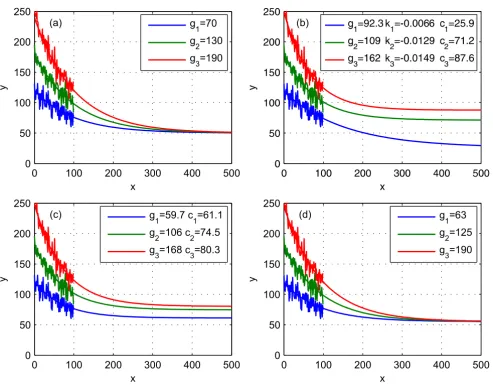
We have N = 3 curves described by the equations y(x) = g_i e-kx _{+ c (i = 1 ... 3) which are degraded by added normally}

distributed noise to simulate the measurement process (left part of figure 1(a)). The task is to retrieve the param-eters used to create the curves by only using the degraded values for 0 ≤ x < 100. When the three curves are fitted sep-arately, one obtains three values of each parameter g, k and c (figure 1(b)).

The fit method we are introducing here is able to fit these

parameters k and c are shared. Therefore it returns only one value for k and one value for c (figure 1(d)). The following equations were used for fitting:

y₃(x) = g₃ e-kx _{+ c (1)}

y₂(x) = g₂ e-kx _{+ c (2)}

y₁(x) = g₁ e-kx _{+ c (3)}

In this example, the vector of the fit-parameters a was

Example task

Figure 1

Example task. Three curves of the form y = g_i ekx _{+ c were created (a) with k = -0.01 and c = 50. Then the range between x =}

0 and x = 99 was taken and noise was added. The task for the fit methods was to extract the original parameters using only this noisy part. It was done by (b) fitting each curve separately with y = + c_i, (c) taking the introduced fit method with shared k (y = giekx + ci where k was determined to be -0.0137) and (d) with shared k and c (y = giekx + c where k and c resulted in

-0.0107 and 55.2 respectively).

(a) (b)

(c) (d)

a₁ = k a₂ = c a₃ = g₁ a₄ = g₂ a₅ = g₃

Figure 1(c) shows the result when using this algorithm with shared k only.

Principle of the algorithm

The basic idea is the following: When fitting one curve to one equation, the goodness of the fit parameter χ2 _(weighted

sum of the quadratic deviations of the values – definition follows) is minimised. To fit N curves to N equations simultaneously, the sum of the individual χ2 _{values has to}

be minimised. Definitions:

• N ... Number of equations/curves. Each curve is repre-sented by one equation.

• A(n) ... Number of the nodes belonging to the nth meas-ured curve.

• (x_ni, y_ni, ) ... node number i of the nth curve (i = 1 ...

A(n)). σ2 _{is the uncertainty and can be set to 1 if it is}

iden-tical for all nodes of all measurements.

• M ... Total number of parameters that should be deter-mined with the fit.

• a = (a₁, ..., a_M) ... M element vector of the fit-parameters a₁ to a_M.

• y_n(x, a) ... nth equation. It can use all fit parameters a, but there are three possibilities the nth equation could use every single parameter a_m:

1. The equation is independent of a_m. Then the (in the fol-lowing needed) partial derivation of the equation accord-ing to this parameter a_m is zero.

2. a_m is a "normal" fit-parameter, that should be opti-mised.

3. The equation depends on a_m, but should not partake in the optimisation. This is done by setting the partial deri-vation for this parameter to zero.

The total sum of the goodness of the fit parameter χ2 _is

defined as sum of the goodness of the fit parameters

of each curve. The bigger χ2_{, the worse the fit:}

Method for linear functions

If all equations y_n(x, a) are linear in the parameters a, we can use the least square fit method [1] to minimise the total χ2_{. In this case, the equations y}

n(x, a) have to be of

the following form:

f_nm(x) are arbitrary functions. Note that a polynomial function is a special case of this where f_nm(x) has e.g. the form f_nm(x) = xm_{. To get the values for a, the value of} χ2 _is

minimised by setting the derivations according to each parameter ak to zero:

In this way one gets M linear equations (k = 1 ... M) to determine the M entries of a. Equation 10 may look com-plicated, but all values except a_m are explicitly known. The equation can be solved by the method of determinants.

The advantages of the least square method over all non-linear methods are very fast processing, final results in one step and no need to specify starting parameters.

Method for nonlinear functions

If the equations y_n(x, a) depend on some of the parame-ters a in a non-linear way, the requirement to use the least square fit method is not met. In this case, one of the fastest methods to minimise χ2 _{is the Marquardt-Method [2], an}

iterative numerical process. Here it is adapted to fit N curves simultaneously. We use the Marquardt method here, because some of the ideas that are described later require non-linear fitting. The following description can be considered a recipe. For the mathematical background of the Marquardt-Fit-Method, see [1,2].

σni2

χn2

χ2 χ2

1 4 =

( )

=

∑

n n N χ σ n ni i A n

ni n ni

y y x

2 2 1 2 1 5 = −

( )

=

∑

( ) ( ( , ))a

y x_n a f_{m nm} x

m M

( , )a = ( )

( )

=

∑

1 6 ∂ ∂ = − − ∂ ∂ = =

∑

∑

χ σ 2 2 1 1 1 2 1

a y y x

y x a

k i ni

A n

n N

ni n ni n ni

k

( )

( ( , ))(a ) ( , )a == ( )

! 0 7 ⇒ − ⎛ − ⎝ ⎜⎜ ⎞_⎠⎟⎟ ∂∂ = =

∑

= =

∑

∑

2 1₂

1

1i σni 1 1

A n

n N

ni m nm ni

m M m k m M

y a f x a a ( )

( )

∑

∑

fnm(xni)=0 ( )8

⇒ ⎛ −

⎝

⎜⎜ ⎞_⎠⎟⎟ =

(

=

=

∑

=

∑

1

∑

0 9

2 1

1i σni 1

A n

n N

ni m nm ni

m M

nk ni

y a f x f x

( )

( ) ( )

))

⇒ =

=

= ∑ = = =

∑ 1 ∑ ∑ 1

2 1

1i σni 1 1 1σ2

A n

n N

ni nk ni m m M ni i A n nm n M

y f x a f

( ) ( )

1. Calculate χ2 _{with suitable starting parameters a with}

equations (4) and (5).

2. Set λ to 10-3_.λ _{is a constant factor that controls whether}

the Marquardt-Fit-Method should behave more as a gradi-ent search fit method (λ <<> 1) or an expansion fit method (λŬ 1).

3. Calculate the vector δa, which has the same size as a (namely M elements) and describes the suggested correc-tion to a as follows:

(a) The M element vector β represents the first partial der-ivations of χ2 _{to the fit parameters described by a:}

(b) The M × M Matrix describes the second partial der-ivations to the fit parameters a_k and a_m (k and m vary from 1 to M respectively):

(c) Calculate the matrix α by multiplying each diagonal element from by (1 + λ).

(d) Determine the inverse matrix ε of α. (e) Calculate δa as follows:

4. Derive new trial-fit-parameters a' from the "old" ones a:

a' = a + δa (14)

5. Determine χ'2 _{with the trial-fit-parameters a' using}

equations (4) and (5 and (5)).

6. If χ'2 ≥χ2 _{(i.e. there is no improvement with the}

trial-fit-parameters): Substitute λ with 10·λ, keep a unchanged, and continue with step 3.

7. If χ'2 _<χ2 _{(i.e. the new parameters are better): Substitute}

λ with λ/10, and a with a' and continue with step 3. This iterative calculation may be stopped when one of the

β χ

σ

k

k i ni

A n

n N

ni n ni n ni

a y y x

y x

: ( ( , )) ( , )

( )

= − ∂

∂ = −

∂ ∂ =

=

∑

∑

1 2

1

2

2 1 1

a a

a

a_k ( )11

αα

α χ

σ

km

k m i ni

A n

n N

n ni k

n ni

a a

y x a

y x

: ( , ) ( ,

( )

= ∂

∂ ∂ ≈

∂ ∂

∂ =

=

∑

∑

1 2

1

2 2

2 1 1

a aa_j

m

a

)

∂ ( )12

αα

δa_m β ε_{k km}

k N

=

( )

=

∑

1

13 Results of the example task

Figure 2

Results of the example task. Results of the example task shown in figure 1: The task was done 1000 times with other noise signals. The distribution of the obtained parameters is shown here as box and whisker plots. The dashed lines show the tem-plate values. (a) distribution of g₁. (b) distribution of g₂. (c) distribution of g₃. (d) distribution of k. (e) distribution of c.

(a) (b) (c)

• χ2 _{falls below a certain predefined threshold.}

• The difference between χ2 _and χ_'2 _{decreases to less than}

a specified value.

• The count of the calculation loops exceeds a maximum number.

Note: Using this method, one has to treat "constant" parameters (parameters that do not participate in the fit-ting process) in a special way (and not within a having derivations of zero), because otherwise their value may be biassed to minimise χ2_{. This could be done by an extra}

parameter for yn(x, a) (e.g. called b) or by incorporating

the constant parameters within the functions y_n(x, a).

Comparsion to single fits

The benefit of parameter-sharing is that all retrieved val-ues (not only the shared ones) are more precise compared to fitting them separately. To verify this, 1000 fits of the simulated "measurement" from the example above had been made with the following three methods: single fits, simultaneous fits with shared k and simultaneous fits with shared k and c. For every fit, a "new" noise was used. The distributions of the parameters obtained with the three different methods are shown in figure 2: The smallest deviation from the real parameters were obtained by the fits, where k and c were shared.

Use with cochlear implant ECAP measurements

Cochlear implants are medical devices that enable deaf people to perceive hearing impressions by electrically stimulating the auditory nerve [3]. The stimulations occur through a multichannel electrode that is placed directly into the cochlea and has contacts on different positions. This way, up to 100% speech recognition can be achieved [4].

Modern cochlear implants can record the evoked com-pound action potential (ECAP) of the auditory nerve. This is done by measuring the voltage at one of the contacts of the multichannel electrode after a stimulation pulse that evokes the action potentials. The recordings obtained show the sum of the ECAP and exponential decays result-ing from residual charges (arisresult-ing from capacitive compo-nents on the implant itself or from the electrode-electrolyte transition). There are several well established recording methods to eliminate or reduce this so called artefact to obtain the pure ECAP: Alternating stimulation [5], masker probe methods [6,7], triphasic stimulation [8] and scaled template methods [9]. However, each method has its limitations: Some of them rely on the linearity of the system (alternating stimulation), others need up to between nine to sixteen times more measurements for one result (masker probe methods).

Another issue is the influence of the used measurement system itself, which may be seen on the measured curves as offsets, drifts, additional exponential decays, ... (called system effects here).

The introduced method can be used as a tool to help sep-arate the ECAP signal from these undesired components. One way to do so is to fit just the artefact (without the ECAP) along with the system effects and subtract this fit from the measurements. This can be done with sub-threshold measurements, recovery measurements, or in regions, without an ECAP. Another possibility is to com-bine this method with an artefact cancellation method mentioned above, for example to eliminate system effects.

The algorithm needs sequences with different conditions to gain advantage over single-curve-fits. In practical use this is no disadvantage, because usually two special sequences are measured: The amplitude growth sequence and the recovery sequence. The amplitude growth sequence raises the stimulation pulse amplitude from zero to the maximum comfortable loudness (MCL) level. The recov-ery sequence sends two MCL level pulses before the meas-urement – if the second pulse lies within the auditory nerve recovery time of the first pulse (about < 1 ms), the ECAP vanishes.

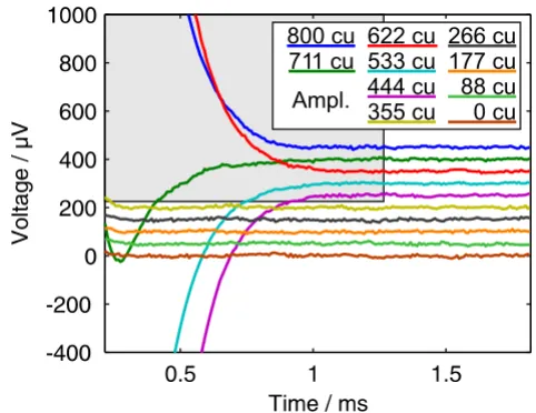
Amplitude growth measurement result

Figure 3

Amplitude growth measurement result. Data from an Amplitude Growth measurement with the MedEl

PULSARCI100 _{cochlear implant. For each curve, 50 cathodic/} anodic pulses were averaged. The pulses had an amplitude between 0 and 800 cu (1 cu ≈ 1 μA). Their begin is the time origin.

800 cu 711 cu

Ampl.

622 cu 533 cu 444 cu 355 cu

Example ECAP measurement

Figure 3 shows the results of an ECAP measurement using the amplitude growth sequence with ten amplitudes between 0 and 800 cu (current units, 1 cu corresponds nominally to 1 μA). It was recorded with the MedEl PULSARCI100 _{cochlear implant and the software}

ArtRe-search. Biphasic pulses beginning with the cathodic phase

were used. For each of the ten curves, 50 recordings were taken and averaged. We intentionally chose an ECAP measurement with a large artefact and with different offset voltages for each curve to demonstrate the power of the algorithm.

The following equation was used as "model" of the fact plus offset for each curve. We assumed that the arte-fact can be described by two exponentially decreasing terms and one offset parameter.

y(t) = fe-t/τ_{+ ge}-t/T _{+ c (15)}

The final offset c and the amplitudes f and g are different for each curve, but the time constants τ and T are assumed to be global, so that the following a was used. It contains 32 parameters.

a = (τ, T, f₁, g₁, c₁, f₂, g₂, c₂, ..., f₁₀, g₁₀, c₁₀) (16)

As mentioned above, several ideas exist to take advantage of the algorithm. Three of them will be described in the following subsections:

Fit of the regions without an ECAP signal

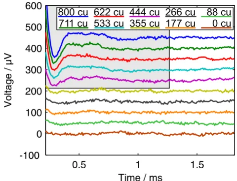
The first possibility is to exclude the regions of the curves where an ECAP signal is expected from the fit. In this example, we included the whole range of the five meas-urements from 0 to 355 cu stimulation amplitude that are sub-threshold (figure 3), and the right part of the other five measurements, where the ECAP signal (duration of about 1 ms [10]) has vanished.

The run time of the algorithm was about one minute (interpreted Matlab™ code with no attempts to speed it up), calculating the fitted values for the 32 parameters. As expected, straight lines were obtained for the fitted regions when subtracting the fit from the original data, indicating a tight fit (figure 4). The returned values for the time con-stants were: τ = 322 μs and T = 138 μs. What we could not expect was that the fit was good for the regions that did not partake in the fitting process, because those regions of the fit where g₆ to g₁₀ (the factors for the fast exponential function) could be determined properly were excluded from the fit as described before.

These patient specific time constants describe mainly the electrical properties of the electrode-electrolyte interface [11] and the geometry, and could be taken as diagnostic parameters along with the ECAP amplitude or the residual voltage measured in telemetry measurements.

If the ECAP signal is small compared to the amplitude of the exponential decay, a good guess of f₆ to f₁₀ and g₆ to g₁₀

Data minus fit

Figure 4

Data minus fit. This figure shows the same data as in figure 3 but with a fit subtracted. The selected region was excluded from the fit. The lines were plotted with an offset of 50 μV each. Details in text.

800 cu 711 cu

Ampl.

622 cu 533 cu 444 cu 355 cu

266 cu 177 cu 88 cu 0 cu

Additional fit

Figure 5

Additional fit. Same as figure 4 with additional fit to obtain values for the parameters that describe the fit within the region that was excluded for the first fit. The lines were plot-ted with an offset of 50 μV each. Details in text.

444 cu 355 cu 622 cu

533 cu 800 cu

711 cu

266 cu 177 cu

coefficients are kept constant. We have done so in keeping

τ and T constant whereas the other parameters were calcu-lated for the five "high current" curves. The result of this is shown in figure 5.

A remark on the starting parameters: The method we used to get the starting parameters was to fit the curves with a simplified model having only one exponential term (with shared time constant) and taking into account only the right halves of the curves. In this way we obtained values for the long time constant τ, f_i and c_i. We then subtracted the fits of this simplified model from the curves and fitted again, using only one exponential term with a shared time constant T and taking into account the whole curve. After that we got starting values for g_i and T. These additional fits needed only a few seconds calculation time.

Using σ2 _{to fit over all regions}

Instead of first excluding the parts of the curves with an ECAP signal and then fitting over all regions where some of the previously determined parameters are kept con-stant, we could initially fit over all regions and use the uncertainty parameter σ2 _{(see section "Principle of the}

algorithm") to characterise regions where the ECAP signal is expected: These regions should receive a high σ2 _value

compared with the σ2 _{value from the other regions, so that}

the fitting algorithm doesn't punish the ECAP caused deviations with a high contribution to the χ2 _value.

The more of the following conditions are satisfied, the better the results from this approach:

• The ECAP amplitude is small compared to the ampli-tude of the artefact.

• There is a region before and after the ECAP-part of the curve that is described by the artefact model used.

• The ECAP signal is dc-free, i.e. the integral over the ECAP signal (without any artefact) is very small.

• The artefact time constants are larger than the ECAP time constants.

Figure 6 shows the results of this variant when using σ2 ₌

10 instead of 1 within the selected areas where the ECAP signal is expected. The retrieved values for τ and T were 328 μs and 176 μs.

Using an ECAP model to fit over all regions

A further approach is to model not only the artefact, but the ECAP signal too. [12] would be an example for a model that could be used. This model takes into account the double-peak shape of some ECAPs as well. Doing so is part of current investigation and may be published in the future.

Conclusion

The introduced fit-algorithm uses the additional informa-tion of the relainforma-tion between measured curves to retrieve more accurate parameters compared to the parameters extracted from single fits. In the case of ECAP measure-ments the algorithm could be used as (additional) artefact cancellation method with the following benefits:

• There are no additional measurements necessary to apply this method.

• The method can be used in combination with other arte-fact cancellation methods.

• It can take into account implant specific system effects.

• Physiological or implant specific parameters like time constants or the artefact amplitude are gained as values that can be used for diagnostic purposes.

• No additional noise is added.

• It is very flexible because of the possibilities to judge dif-ferent regions of a curve and difdif-ferent curves in special ways with the σ2 _{parameter (e.g. curves with zero pulse}

amplitude fit some of the parameters very accurately), leave out data which should not be included in the fit (e.g.

Influence of σ2

Figure 6

Influence of σ2_{. Data from figure 3 minus fit where the} σ2 value of the selected area was 10 instead of 1. The lines were plotted with an offset of 50 μV each.

444 cu 355 cu 622 cu

533 cu 800 cu

711 cu

266 cu 177 cu

Publish with BioMed Central and every scientist can read your work free of charge

"BioMed Central will be the most significant development for disseminating the results of biomedical researc h in our lifetime."

Sir Paul Nurse, Cancer Research UK

Your research papers will be:

available free of charge to the entire biomedical community

peer reviewed and published immediately upon acceptance

cited in PubMed and archived on PubMed Central

yours — you keep the copyright

holes where the ECAP is expected), use different equa-tions for different curves (e.g. combining results of ampli-tude growth and recovery sequences), and exclude parameters of some curves from the fit process (e.g. time constants in curves with ECAP).

• Constant parameters (time constant, offset, ...) can be reused (at least as starting parameters) to save calculation time.

The drawbacks are that the calculation can be time-con-suming (especially with many fit parameters) and that there have to be suitable starting parameters. The first issue can be improved by reducing the resolution of the curves to receive a rough result, and optimising the stop condition for the calculation loop to fit the problem. The second issue can be dealt with by reusing parameters from earlier runs, or by determining them by doing rough pre-fits with less complicated equations.

Further investigation is necessary to develop a final method based on the introduced ideas. ECAP signals obtained with this method should be compared in size and shape with results of traditional artefact cancelation methods.

Authors' contributions

PS developed the basic method and wrote the draft of the publication. It was discussed, criticised, and partly rewrit-ten to clarify the presentation together with EH and CZ. They had the idea of the comparison with the straight for-ward approach of fitting the curves separately by doing simulated measurements.

Acknowledgements

The authors would like to thank the MedEl company for their help and for providing the new PULSARCI100 _{implant and Hansjörg Schösser for being} the contact person for implant related questions.

References

1. Bevington PR, Robinson KB: Data Reduction and Error Analysis

McGraw-Hill; 2003.

2. Marquardt DW: An algorithm for Least-Square Estimation of Nonlinear Parameters. Journal of the Society for Industrial and Applied Mathematics 1963, 2(2):431-441.

3. Hochmair ES, Hochmair-Desoyer IJ, Zierhofer CM: Electronic Cir-cuits for Cochlear Implants. AEÜ – International Journal of Electron-ics and Communications 1990, 44:.

4. Helms J, Muller J, Schon F, Moser L, Arnold W, et al.: Evaluation of performance with the COMBI40 cochlear implant in adults: a multicentric clinical study. ORL J Otorhinolaryngol Relat Spec

1997, 59:23-35.

5. Eisen MD, Franck KH: Electrically Evoked Compound Action Potential Amplitude Growth Functions and HiResolution Programming Levels in Pediatric CII Implant Subjects. Ear & Hearing 2004, 25(6):528-538.

6. Brown C, Abbas P, Gantz B: Electrically evoked whole-nerve action potentials: data from human cochlear implant users. The Journal of the Acoustical Society of America 1990, 88(3):1385-1391. 7. Miller CA, Abbas PJ, Brown CJ: An improved method of reducing

8. Zimmerling M: Messung des elektrisch evozierten Summenak-tionspotentials des Hörnervs bei Patienten mit einem Coch-lea-Implantat. In PhD thesis Universität Innsbruck, Institut für Angewandte Physik; 1999.

9. Miller CA, Abbas PJ, Rubinstein JT, Robinson B, Matsuoka A, Wood-worth G: Electrically evoked compound action potentials of guinea pig and cat: responses to monopolar, monophasic stimulation. Hearing Research 1998, 119(1–2):142-154.

10. Klinke R, Silbernagl S: Lehrbuch der Physiologie Stuttgart: Thieme; 2003. 11. Geddes L: Historical evolution of circuit models for the elec-trode-electrolyte interface. Annals of Biomedical Engineering 1997,

25:1-14.