Group to Study Open Quantum Systems
Cheng Guo
Group to Study Open Quantum Systems
Cheng Guo
Dissertation
an der Fakult¨
at f¨
ur Physik
der Ludwig–Maximilians–Universit¨
at
M¨
unchen
vorgelegt von
Cheng Guo
aus Linyi
Zweitgutachter: Prof. Ulrich Schollw¨
ock
Contents
Abstract vii
Zusammenfassung viii
1 Introduction 1
2 DMRG, NRG and VMPS 5
2.1 NRG . . . 5
2.1.1 Logarithmic discretization . . . 5
2.1.2 Iterative diagonalization of the Wilson chain . . . 7
2.2 Traditional DMRG . . . 10
2.2.1 Infinite DMRG . . . 11
2.2.2 Finite DMRG . . . 14
2.2.3 Calculation of physical quantities . . . 14
2.3 Time-dependent DMRG . . . 16
2.4 VMPS . . . 18
2.4.1 Matrix product state . . . 19
2.4.2 Variational matrix product state . . . 21
3 Landau-Zener problem 27 3.1 The standard Landau-Zener problem . . . 27
3.2 Publication: DMRG study of a quantum impurity model with Landau-Zener time-dependent Hamiltonian . . . 28
4 One- and Two-Bath Spin-Boson Models 35 4.1 Publication: Critical and Strong-Coupling Phases in One- and Two-Bath Spin-Boson Models . . . 36
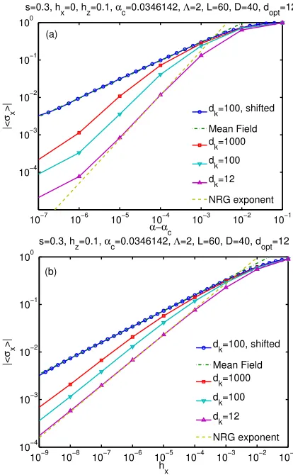
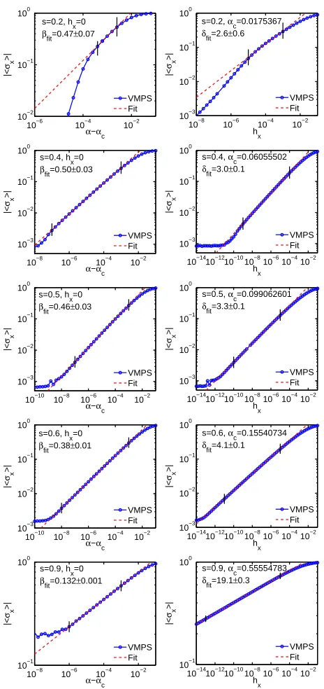
4.2 Additional results on determining αc and critical exponents . . . 53
4.3 Exploration of the power-law discretization . . . 54
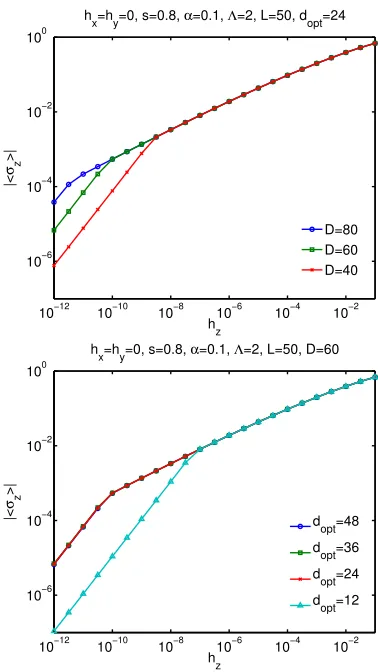
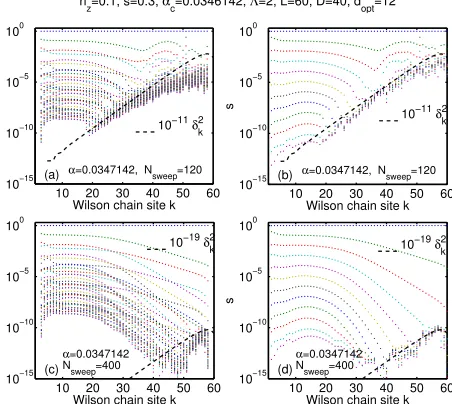
4.4 Dynamical determination of the local dimension . . . 58
4.5 The folded chain setup of SBM2 . . . 60
4.6 Symmetries . . . 63
4.6.2 Symmetry breaking in VMPS ground state . . . 64
4.6.3 Implementation of parity symmetry . . . 65
4.6.4 U(1) symmetry in SBM2 . . . 66
4.7 Energy flow diagrams . . . 66
4.8 MPS block entropy . . . 69
4.9 Convergence criterion and further improvement of the algorithm . . . 69
4.10 Follow up study of SBM2 . . . 72
5 Quantum Telegraph Noise Model 75 5.1 Decoherence . . . 75
5.2 Spin echo . . . 80
5.3 Spectroscopy of periodic drive . . . 80
A ˇZitko-Pruschke logarithmic discretization of boson bath 85 B Overlap of two VMPS wave functions with different shifts 87 C Snake - a DMRG program 89 D Bosonic VMPS program 93 E List of Abbreviation and Frequently Used Symbols 97 E.1 List of Abbreviation . . . 97
E.2 List of Frequently Used Symbols . . . 98
Abstract
This thesis is concerned with open quantum systems, and more specifically, quantum impu-rity models. By this we mean a small local quantum system in contact with a macroscopic non-interacting environment. This can be used to model individual impurities in metals and quantum information systems where the influence from the surrounding environment is not negligible. The numerical renormalization group (NRG) is the traditional method to study quantum impurity models. However its application is limited when dealing with real-time dynamics and bosonic systems. In recent years some of NRG’s techniques have been introduced to the density matrix renormalization group method (DMRG), which itself is the most powerful numerical method to study one-dimensional quantum systems. The resulting method shows great potential, and this thesis explores and extends the power of the NRG+DMRG combination in treating open quantum systems.
Zusammenfassung
Diese Dissertation handelt von offenen Quantensystemen, mit Spezialisierung auf Quan-tenst¨orstellenmodelle. Diese sind kleine lokale Quantensysteme, die im Kontakt mit einer makroskopischen nichtwechselwirkenden Umgebung stehen. Sie sind n¨utzlich, um einzelne St¨orstellen in Metallen und Quanteninformationssystemen zu untersuchen, bei denen der Einfluss der Umgebung nicht vernachl¨assigbar ist, und deren Beschreibung im Falle einer starken Ankopplung ¨uber eine einfache perturbative Beschreibung hinausgeht. Die nu-merische Renormierungsgruppe (NRG) ist eine Standardmethode f¨ur die Untersuchung von Quantenst¨orstellenmodellen. Allerdings kann sie nur begrenzt auf dynamische Systeme und Systeme von Bosonen angewendet werden. In den letzten Jahren wurden einige NRG Methoden auf die Dichtematrix Renormierungsgruppe (DMRG) ¨ubertragen – eine m¨achtige quasi-exakte numerische Methode f¨ur die Untersuchung eindimensionaler Systeme. Die Kombination beider Methoden (NRG+DMRG) bietet daher einen breiten starken Rah-men, der in dieser Dissertation auf offene Quantensysteme angewendet wird.
Der Schwerpunkt liegt dabei auf zwei Arten von Problemen. Der erste Schwerpunkt bezieht sich auf offene Quantensysteme. Dies spielt eine wichtige Rolle in der theoretis-chen Beschreibung von Problemen in Bezug auf qubit Manipulation. Wir kombinieren die NRG Diskretisierung und die adaptive zeitabh¨angige DMRG (t-DMRG), um das dissipa-tive Landau-Zener Problem zu untersuchen. Wir nutzen diese Methode ebenfalls, um die Quantendekoh¨arenz und dynamische Eigenschaften von Telegraphrauschmodellen zu unter-suchen. Die Ergebnisse belegen, dass die NRG und t-DMRG Kombination eine schnelle, genaue und vielseitige Methode f¨ur solche Probleme darstellt. Der Zweite Schwerpunkt handelt von kritischen Quanteneigenschaften von Spin-Boson Modellen mit einem, bzw. zwei B¨adern. Anders als bei fermionischen und Spinmodellen ist es schwierig, Modelle mit Bosonen numerisch zu beschreiben, da jedes Boson bereits eine unendliche Anzahl an Zust¨anden hat. Indem wir die optimale Bosonenbasis in eine Art von DMRG, die variationelle Matrixproduktzustandmethode (VMPS), einf¨uhren, k¨onnen wir eine effektive lokale Bosonenbasis der Gr¨oßenordnung 1010 erreichen. Dies ist eine enorme Verbesserung
Chapter 1
Introduction
An open quantum system is a general term that describes a quantum system interacting with an effective non-interacting macroscopic environment. If the quantum system com-prises only a small number of degrees of freedom, it is also called a quantum impurity system or dissipative quantum system depending on the nature of the system or the per-spective of the study. Fig. 1.1 shows two scenarios of open quantum systems: the magnetic impurity inside a metal which causes the Kondo effect [5, 47] and the experimental setup of a quantum bit which suffers from environmental noises [17]. Many theoretical models have been proposed to describe open quantum systems, such as the Kondo model, the Anderson impurity model [5] and some models we will study in this thesis, namely the res-onant level model [33, 52], the spin-boson model [52] and the telegraph noise model [67]. These open quantum models play an important role in many branches of modern physics like condensed matter physics, quantum information theory, quantum optics, quantum measurement theory, etc.
There are numerous theoretical techniques to study these open quantum models such as perturbation theory, density matrix theory, Green’s functions etc. However due to the many-particle nature of the full system, except for a few of the simplest models, analytical methods often involve approximations which either restrict their usage to some special cases or may make it difficult to differentiate features from the model itself or from the approximations made during the analytical study. Therefore a generally applicable, first principle numerical method is desirable as an alternative to the analytical approach to understand the diverse problems commonly encountered in the research area of nano-technology and quantum information. This is the direction I will try to explore in my thesis.
(b)
(a)
Temperature (K)
Figure 1.1: Two scenarios of open quantum systems. (a) The coupling between the magnetic impurity with the conduction electrons inside a metal causes the Kondo effect which appears macroscopically as a logarithmic increase of resistivity at very low temper-ature. The figure is from Ref. [22]. (b) Scanning micrography of a superconducting flux qubit. Similar experimental realizations of qubits all suffer from the destructive noise of the surrounding environment. The image is from Ref. [17].
In addition to its numerical nature, NRG also provides an extremely systematic approach to quantum impurity models through its innovative approach based on renormalization. Finite-size spectra as well as fixed-point spectra can be used to drive effective models which are again amenable to analytical work.
Even though NRG has been successfully extended to study many other open quantum systems it is not applicable to one-dimensional real-space lattices. Twenty years after the invention of NRG Steven R. White, who was a PhD student of Wilson, proposed a new numerical method – the density matrix renormalization group method (DMRG), to solve one-dimensional lattice systems [105, 103]. Though inspired by NRG, the idea behind the new method was very different. In fact as was only made clear later, unlike NRG it is not a true renormalization group method, but a variational one instead.
DMRG quickly became popular because of its unprecedented accuracy to study the ground state and low lying states of 1D quantum lattice systems [109, 84, 71, 8, 68, 41, 58]. It has also been extended in two directions: one is to dynamical properties [34, 72, 49, 40] and thermodynamical properties [13, 99]; the other is to generalize DMRG to other systems such as 2D or 3D systems [62, 106, 36, 114], to momentum space [113, 61], or quantum chemistry systems [26, 104, 21]. The performance of DMRG in these systems is not as good as on simple real space 1D lattice systems. However, it serves as an inspiring starting point of a new generation of algorithms to deal with more complicated systems, collectively know as tensor network methods [56, 94, 92, 93, 53, 32, 88, 44, 78, 25, 54, 42, 115]. The field it has opened is one of the most exciting areas in condensed matter physics, quantum information and even high energy physics [73, 86].
method (VMPS) [66, 89, 91, 69].
VMPS has a clear mathematical structure. While DMRG experts use VMPS language to understand some theoretical aspects of DMRG, physicist in the field of quantum in-formation also started using MPS framework to study problems related to the classical simulation of quantum systems. There “classical simulation” means to use a classical computer to simulate, or in the language of computational complexity theory, to use a deterministic Turing machine to simulate. By studying the classical simulation of quan-tum systems, one can understand better the advantage of quanquan-tum computers [27, 23]. If there exist algorithms for classical computers to simulate any quantum systems efficiently (in polynomial time), then the advantage of quantum computers over classical computers would vanish and the computational complexity class BQP (bounded error quantum poly-nomial time) would be equal to P (polypoly-nomial time). Otherwise, those quantum systems turn out to be difficult to simulate on classical computers, and would be good candidates to harness the power of quantum computing.
In 2003, Vidal proposed the time-evolving block decimation algorithm (TEBD) [94], and proved that any quantum system with a limited amount of entanglement could be simulated with TEBD. Therefore, one should choose those highly entangled quantum systems to build a quantum computer. Interestingly on the other hand, lots of systems in condensed matter physics are only weakly entangled according to TEBD’s standard, which means TEBD could be used to simulate the dynamics of such systems. Daley et al. and White et al. incorporated TEBD into DMRG, and proposed the adaptive time-dependent DMRG (t-DMRG) [20, 108] to simulate the real-time dynamics of quantum 1D system with nearest neighbor interactions.
MPS is not only a bridge between quantum information and condensed matter physics, it also connects two powerful numerical methods mentioned above: NRG and DMRG. In 2005, Weichselbaum et al. showed that NRG can also be formulated in the MPS representation and it shares lots in common with DMRG in this language [100]. This is a key argument why we could use DMRG/VMPS to study quantum impurity models.
A key benefit to use DMRG to study open quantum systems is that we can directly apply t-DMRG and other existing DMRG techniques. NRG has also been extended to study the dynamics of open quantum systems (TD-NRG) [3], but it is only restricted to the quenched type time-dependence of the Hamiltonian while t-DMRG can treat the Hamiltonian with arbitrary time-dependence. The second benefit is that DMRG/VMPS uses a variational approach to calculate the ground state, which makes it more flexible to explore new ideas. More specifically, in this thesis only the use of DMRG/VMPS allowed us to employ non-logarithmic discretization and the optimal boson basis, which were crucial to the success of the projects presented in this thesis.
Chapter 2
DMRG, NRG and VMPS
In this chapter I will review the numerical methods used in this thesis. As there are already extensive reviews for each of these methods, the main purpose of this chapter is not to cover every aspect of these methods, but rather to concentrate on the most essential and relevant parts to make the thesis self-contained. I will first introduce NRG, DMRG and t-DMRG separately and then introduce the matrix product state representation to connect NRG and DMRG within the framework of VMPS.
2.1
NRG
The Numerical Renormalization Group (NRG) [110, 48, 9] is a very general method to study open quantum systems. There is no restriction on the nature of the impurity (sys-tem). Regarding the bath (environment), it can be fermions, bosons or both; it can be one-, two- or three-dimensional. NRG does have one restriction on the bath: it should consist of effective noninteracting particles. For a noninteracting bath, the real dimension is irrelevant because its degree of freedom can be integrated out and all the relevant bath properties to the impurity are captured in the spectral function of the bath ∆(ω), with the energy ω its only remaining parameter. NRG coarse-grains the continuous bath spectral function logarithmically, maps this onto a semi-infinite chain of sites with exponentially decaying coupling, then diagonalizes the Hamiltonian of the whole system iteratively. In the following I will explain these steps in detail.
2.1.1
Logarithmic discretization
dis-cretization (with large enough logarithmic disdis-cretization parameter Λ defined in Eq. 2.1) separates consecutive energy scales, so that discarded high-energy states of a given NRG iteration have limited effect on the following iterations.
Suppose the band-width of the bath is [−1,1], in other words the bath spectral function is defined in the interval [−1,1] and all energies are taken in units of the bandwidth. Ac-cording to logarithmic discretization, we discretize the band in energy space by consecutive intervals determined by the following positions
ωn=±Λ−n, n = 1,2,· · · , (2.1)
where Λ>1 is a dimensionless parameter, called the logarithmic discretization parameter. The width of each energy levelθn =|ωn+1−ωn|is 1/Λ of the previous level, so we get finer and finer energy resolution when we approach ω = 0. The spectral function of a bosonic bath is defined in [0, ωc]. Usually the cut-off frequencyωc is set to 1 as the unit of energy.
For the bosonic bath we only use the positive part of Eq. (2.1).
After cutting the continuous spectral function into slices we calculate the effect of each of them on the impurity. Clearly, using a single energy level to represent a whole energy slice, is a crude approximation for high energy slices as they cover a wide range of energies. Nevertheless it is still used because NRG is traditionally a tool to study the low temperature properties where the most important part of the bath spectral function lies at small energies around ω = 0. When one does need to represent the high energy part of the band properly, one can resort to the “z-averaging” technique to improve this approximation [98]. The basic idea behind this is a shift in the discretization of Eq. (2.1), with an additional parameter z,
ωn=±Λ−n+z, n= 1,2,· · · , z ∈[0,1). (2.2)
For each choice ofz we cut the band at different positions, and whenz = 0 it is equivalent to Eq. (2.1). One can chose several equality spaced z values and calculate the problem separately, after which an averaging of the independent results is performed to reduce the artifacts caused by the inaccurate representation of the band especially at the high energy part. Thus the method got the name “z-averaging”.
As the most important part of this thesis refers to the spin-boson model, I will use it as an example in the following. The original continuous Hamiltonian is
H =Hloc+ Z 1
0
ωa†ωaωdω+ σz
2
Z 1
0
[ρ(ω)]1/2λ(ω)(aω+a†ω)dω, (2.3)
where
Hloc=−∆ σx
2 +
σz
2 (2.4)
describes the local Hamiltonian. (∆) stands for the Zeeman splitting in an actual magnetic field in the z- (x-) direction. ρ(ω) is the density of states, and λ(ω) describes the coupling strength between the spin and the bath. By definition, its relation to the bath spectral function is
The boson operators a†ω and aω satisfies commutation relation
[aω, a
†
ω0] =δ(ω−ω
0
). (2.6)
The effect of the bath on the impurity is fully determined by the spectral function J(ω). Therefore, we are free to choose an arbitrary form of density of states ρ(ω) and the cor-responding λ(ω) as long as Eq. (2.5) is satisfied. The integrals in the Hamiltonian. (2.3) can be carried out in each energy intervals. With this, we transform the Hamiltonian (2.3) into the discretized form
H =Hloc+
∞
X
n=0
ξna†nan+ σz
2√π
∞
X
n=0
γn(an+a†n), (2.7)
with
γn2 =
Z Λ−n
Λ−(n+1)
J(ω)dω, (2.8)
ξn =γn−2 Z Λ−n
Λ−(n+1)
J(ω)ωdω. (2.9)
The standard parametrization of the bosonic bath spectral function is
J(ω) = 2παωc1−sωs. (2.10)
The cut-off frequency is set as the unit of energy ωc = 1. Substituting Eq. (2.10) into
Eq. (2.8) and Eq. (2.9) we get:
ξn =
s+ 1
s+ 2
1−Λ−(s+2) 1−Λ−(s+1)Λ
−n
, (2.11)
γn2 = 2πα
s+ 1(1−Λ
−(s+1))Λ−n(s+1). (2.12)
2.1.2
Iterative diagonalization of the Wilson chain
The discretized Hamiltonian Eq. (2.7) is of a “star structure”: the spin couples to boson modes of all energy scales. To adapt to later renormalization step, it is necessary to transform this star structure into a half-infinite chain form with only nearest neighbor interaction. This form is called the “Wilson chain” in NRG.
The star Hamiltonian is in a bilinear form. Therefore we can express the bath and coupling part as a matrix with~a = (σz, a0, a1, a2,· · ·)T as the base vector. Then the star
Hamiltonian is
where the matrix A is
A=
0 γ0
2√π γ1
2√π γ2
2√π · · · γ0
2√π ξ0 0 0 γ1
2√π 0 ξ1 0 γ2
2√π 0 0 ξ2
..
. . ..
. (2.14)
In its matrix form, transforming the Hamiltonian to the Wilson chain mathematically means to tri-diagonalize A. We can use standard numerical routines like Lanczos for tri-diagonalizing a Hermitian matrix. Suppose the resulting tri-diagonal matrix isB, with the corresponding unitary transformation matrixU, then with
A=U†BU, (2.15)
we can define a new set of boson operators
~b≡(σz, b0, b1, b2,· · ·) = U~a, (2.16)
and express the Hamiltonian with the new boson sites as
H = Hloc+~aTA~a
= Hloc+~aTU†BU~a
= Hloc+~bTB~b, (2.17)
or explicitly as
H =Hloc+ r
η0 π
σz
2 (b0+b †
0) +
∞
X
n=0
nb†nbn+
∞
X
n=0
tn(b†nbn+1+b
†
n+1bn), (2.18)
whereη0 = R
J(ω)dω encodes the overall coupling between impurity and bath. The boson energiesnand the hopping amplitudestndecay exponentially as Λ−n. This is characteristic of the bosonic bath. For a fermionic bath, the decay rate is Λ−n/2. Eq. (2.18) is the Wilson
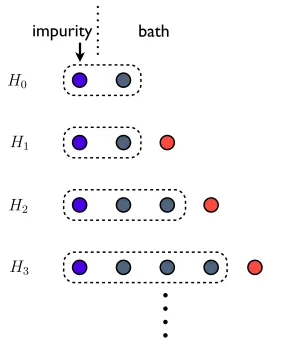
The basic process of NRG is as follows: we can view the Wilson chain Hamiltonian Eq. (2.18) as the limit of a series of Hamiltonians with better and better description of smaller and smaller energy scales
H = lim
N→∞Λ −N
HN. (2.19)
Λ−N is the renormalization rescaling factor, and it makes the energy spectrum of successive
Hamiltonians comparable. The recurrence relation of the Hamiltonian series is
HN+1= ΛHN + ΛN+1[N+1b
†
N+1bN+1+tN(b
†
NbN+1+b
†
N+1bN)]. (2.20)
The first Hamiltonian includes the impurity and the first site of the Wilson chain
H0 =Hloc+ r
η0 π
σz
2 (b0+b †
0) +0b
†
0b0. (2.21)
Fig. 2.1 illustrates the iterative diagonalization of NRG. Starting fromN = 0, we add one site to form the Hamiltonian HN+1 according to Eq. (2.20). It includes rescaling HN by
a factor of Λ (for fermionic bath Λ1/2) and the coupling term to the new added site by a
factor of ΛN+1 (for fermionic bath Λ(N+1)/2). Then we diagonalize the Hamiltonian HN+1
and find all eigenstates. The lowest D states are used as the new combined basis. When the original dimension of HN+1 is smaller than D, all eigenstates will be used as the new
basis of the new block. Given the basis ofHN, and the basis of the added site are |s˜i and |ni respectively, then the new combined states |si are given by
|si=X
˜ sn
As,(˜sn)|s˜i|ni. (2.22)
(˜sn) is the combined column index. Each row of As,(˜sn) represents a kept eigenstate.
Afterwards, we express all the operators of HN+1 in the new basis |si. If we do not use
the truncated new basis, the dimension of the basis will increase exponentially as one adds more and more sites, thus restricting the calculation to very short Wilson chains. The above process is shown in Fig. (2.2).
Connecting the energy levels of each iteration we will obtain the renormalization flow of energy levels. This kind of diagram is called the flow diagram. The pattern of the flow diagram is normally changing through iterations before it finally settles at a fixed pattern which is called the stable fixed point. There can be some iteration regimes in which the pattern of the spectrum in the flow diagram is not changing, and such regimes are called fixed points. The iterative diagonalization of NRG normally stops at the fixed point with the lowest energy scale, that is the stable fixed point. Analyzing the flow diagram and fixed point spectra can reveal much of the underlying physics of the system. As such, it constitutes an important NRG technique.
impurity
bath
H
0H
1H
2H
3Figure 2.1: Illustration of NRG iterative diagonalization. The new HamiltonianHN+1 is formed by adding another site at the end of the previous Wilson chain. The dimension of the effective basis needs to be truncated given a finite amount of numerical resources.
iterations, we would want the energy scale of those discarded states to be separated far away enough from the energy scales of later iterations. For this reason the logarithmic discretization parameter Λ should not be too small, and usually one should use Λ ≥ 2 in NRG. I will also discuss in detail later that when we replace the NRG truncation scheme by DMRG truncation scheme the logarithmic discretization is no longer required.
2.2
Traditional DMRG
HN+1!rs,r
!
s!
"=N+1#r;s$HN+1$r!
;s!
%N+1. !41" For the calculation of these matrix elements it is useful to decompose HN+1 into three parts:HN+1=
&
!HN+XˆN,N+1+YˆN+1 !42"'see, for example, Eq. !36"(, where the operator YˆN+1 contains only the degrees of freedom of the added site, while XˆN,N+1mixes these with the ones contained inHN. The structure of the operators Xˆ and Yˆ, as well as the equations for the calculation of their matrix elements, depend on the model under consideration.
The following steps are illustrated in Fig. 3. In Fig.
3!a"we show the many-particle spectrum of HN, that is, the sequence of many-particle energiesEN!r". Note that, for convenience, the ground-state energy has been set to zero. Figure 3!b" shows the overall scaling of the ener-gies by the factor
&
!; see the first term in Eq. !36".Diagonalization of the matrix Eq. !41" gives the new eigenvalues EN+1!w" and eigenstates $w%N+1 which are related to the basis $r;s%N+1 via the unitary matrix U:
$w%N+1=
)
rsU!w,rs"$r;s%N+1. !43"
The set of eigenvalues EN+1!w" of HN+1 is displayed in Fig. 3!c" !the label w can now be replaced by r". The number of states increases on adding the new degree of freedom 'when no symmetries are taken into account, the factor is the dimension of the basis $s!N+1"%(. The ground-state energy is negative, but will be set to zero in the following step.
The increasing number of states is, of course, a prob-lem for numerical diagonalization; the dimension of
HN+1 grows exponentially with N, even when we con-sider symmetries of the model so that the full matrix takes a block-diagonal form with smaller submatrices. This problem can be solved by a simple truncation scheme: after diagonalization of the various submatrices ofHN+1 one keeps only theNseigenstates with the low-est many-particle energies. In this way, the dimension of the Hilbert space is fixed to Ns and the computation
time increases linearly with the length of the chain. Suit-able values for the parameter Ns depend on the model; for the single-impurity Anderson model, Nsof the order of a few hundred is sufficient to get converged results for many-particle spectra, but the accurate calculation of static and dynamic quantities usually requires larger val-ues of Ns. The truncation of high-energy states is illus-trated in Fig. 3!d".
Such an ad hoc truncation scheme needs further ex-planation. First of all, there is no guarantee that this scheme will work in practical applications, and its qual-ity should be checked for each individual application. An important criterion for the validity of this approach is whether the neglect of high-energy states spoils the low-energy spectrum in subsequent iterations—this can be easily seen numerically by varying Ns. The influence of the high-energy on the low-energy states turns out to be small since the addition of a new site to the chain can be viewed as a perturbation of relative strength !−1/2 "1. This perturbation is small for large values of !, but for !→1 it is obvious that one has to keep more and more states to get reliable results. This also means that the accuracy of the NRG results decreases when Ns is kept fixed and ! is reduced !vice versa, it is sometimes possible to improve the accuracy by increasing ! for fixed Ns".
From this discussion, we see that the success of the truncation scheme is intimately connected to the special structure of the chain Hamiltonian !that is, tn# !−n/2" which in turn is due to the logarithmic discretization of the original model. Note that a mapping to a one-dimensional chain can also be performed directly for a continuous conduction band, via a tridiagonalization scheme as described in detail by Hewson !1993a". The resulting chain Hamiltonian takes the same form as Eq.
!26", but withtn→const. For this Hamiltonian, the trun-cation scheme clearly fails. A similar observation is made when such a truncation is applied to the one-dimensional Hubbard model !see the discussion in Sec. V".
EN+1(r)
EN(r) Λ1/2 EN(r)
a)
after truncation
b) c) d)
0
FIG. 3. !a" Many-particle spectrum EN!r" of the HamiltonianHNwith the ground-state en-ergy set to zero.!b"The relation between suc-cessive Hamiltonians, Eq. !36", includes a scaling factor
&!
. !c" Many-particle spectrumEN+1!r" of HN+1, calculated by diagonalizing
the Hamiltonian matrix Eq. !41". !d" The same spectrum after truncation where only the Ns lowest-lying states are retained.
Rev. Mod. Phys., Vol. 80, No. 2, April–June 2008
Figure 2.2: The spectrum of the NRG Hamiltonians during rescaling, shifting and trun-cating. (Figure taken from Ref. [9]). (a) The energy spectrum of HN,EN(r), with ground state energy set to 0. r labels the energy levels. (b) For a fermionic bath, HN is rescaled by a factor of Λ1/2 (for boson by the factor Λ) before adding a new site. (c) The added site causes splitting of the original energy levels. The new ground state is below 0 after the splitting of levels. (d) Truncate the high energy states and keep the lowest D eigenstates only. We use the new ground state as the energy reference and shift all levels up which concludes one iteration.
(VMPS), which I will introduce in the last section of this chapter.
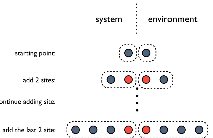
The traditional DMRG method includes two parts: the infinite DMRG (iDMRG) which is used to grow a 1D lattice and finite DMRG (fDMRG) which is used to variationally optimize the ground state of the resulting lattice from iDMRG. iDMRG can be used alone to study an infinite system by analyzing its asymptotic properties when approaching infinite system size. fDMRG is used to study a finite 1D system. fDMRG in its original formulation requires iDMRG to build a chain with certain length L for subsequent optimization.
2.2.1
Infinite DMRG
system
environment
starting point:
add 2 sites:
add the last 2 site: continue adding site:
Figure 2.3: Illustration of the basic steps of infinite DMRG. Red sites are newly added sites at the current step. After adding a new site, the block basis is truncated according the DMRG criteria to prevent the dimension from increasing exponentially.
Similar to NRG, two new sites (shown in red in Fig. 2.3) are added to the two-blocks respectively. The blocks with added sites are called new system block and new environment block. If the basis of the old blocks are |˜si and |e˜i and the basis of a free site is |ni the basis of the new blocks are:
|si = X
n,˜s
Is,(˜sn)|s˜i|ni,
|ei = X
n,˜e
Ie,(n˜e)|ni|e˜i. (2.23)
Here the symbol I means the identity matrix. (˜sn) and (ne˜) are combined indices. If the dimension of the old blocks is D and the dimension of the free site basis is d, then the dimension of the new blocks’ basis will be expanded toDd. Adding more and more sites in this way would result in an exponential increase of the dimension of the basis. Therefore a truncation scheme is again necessary to make the method practical.
it is embedded in the whole system. In other words, targeting the overall ground state of the system and thus a single state, we should keep the eigenstates of the reduced density matrix of the subsystem corresponding to the biggest eigenvalues. This criteria applies both to the system and the environment block.
The representation of the ground state wave function of whole system (or by the DMRG nomenclature the super block) in terms of of the system and environment block is given by
|ψGi=X
s,e
ψGse|si|ei, (2.24)
whereψse is a matrix of the size Dd×Dd. HereD is the dimension of the old system and
environment, and d is the dimension of newly added sites. The reduced density matrices of the two subsystems would be (I use capital letters to indicate the subsystem and lower case letters to label the basis of the subsystems)
ρS = T rE|ψihψ|= X
e
ψse∗ ψs0e|sihs0|, ρE = T rS|ψihψ|=
X
s
ψse∗ ψse0|eihe0|. (2.25)
Therefore after the new blocks are formed, one should first calculate the ground state of the super block. The Hamiltonian of the super block is of the form
Hsup =HS ⊗IE+IS⊗HE +OS ⊗OE. (2.26)
where HS is the Hamiltonian of the system block, IS is the identity matrix , OS is an
operator of the system block. The last term in Eq. (2.26) usually is a sum of several pairs of operators (e. g. c†ici+1 +H.C.), but for simplicity here only one pair is assumed. The
dimension of the super block Hamiltonian is D2d2.
In DMRG we do not expand the super block Hamiltonian explicitly in full because this would be very expensive if all we want is just the ground state (and a few low lying states) of this Hamiltonian. Luckily there are a few sparse matrix diagonalization algorithms such as Lanczos, conjugate gradient or Arnold algorithm which only require a function
~
y=f(~x) =A~x to be able to calculate the ground state of the matrix A. Therefore all we need is to provide the algorithm the function
|φi = Hsup|ψi
= X
s,e
(X
s0
HssS0ψs0e+ X
e0
ψse0HeE0e+ X
s0,e0
OssS0ψs0e0OeE0e)|si|ei (2.27)
= X
s,e
φse|si|ei.
HS
ss0 is the matrix element of the system block Hamiltonian in the |sibasis
HS =X
s,s0
and other matrices are defined similarly.
After we obtain the ground state wave function, we can calculate the reduced den-sity matrices according to Eqs. (2.25). Then we find D eigenvectors with the greatest eigenvalues for both ρS and ρE and use these vectors for the following renormalization transformation
|si = X
n,s
ASs,(˜sn)|˜si|ni,
|ei = X
n,e
AEe,(n˜e)|ni|e˜i. (2.29)
This transformation then replaces Eq. (2.23), and thus truncates the full state space di-mension Dd back down to D. All operators shall be represented in the new system and environment basis. This finishes one iDMRG step and we can add another two sites until we reach the targeted chain length.
When we use DMRG to study a finite chain of lengthL, the ground state from iDMRG is usually not accurate enough. fDMRG can be used to further minimize the ground state’s energy variationally.
2.2.2
Finite DMRG
As illustrated in Fig. 2.4, we start fDMRG based on the final step of iDMRG. The old block information was stored during the previous iDMRG steps and is now read by fDMRG before the first step, which is the same as the last step of iDMRG–we add two site, diagonalize the super block Hamiltonian except we only renormalize the environment block. In the second step we use the new environment block we got from step one and read the stored system block with chain length L/2−2 as the old blocks and then add two sites to them respectively and the rest is just like the previous step until we reach the left most site of the chain. Then we change the sweeping direction while the role of the system and environment are switched. We can sweep back and forth a few times until the results converged. Normally a few sweeps (<10) are sufficient.
2.2.3
Calculation of physical quantities
The ground state energy can be obtained directly from super block diagonalization. Other physical quantities can be calculated as the expectation values of their operator with respect to the ground state. In the DMRG calculation the operator of the desired physical quantity will be renormalized together with other operators like the block Hamiltonian and it is represented in the same basis as the wave function. For example, if the site lies in the system block the operator of the physical quantityA will be represented as
A=X
s,s0
system
environment
starting point:
sweep to left:
sweep to right:
sweep back and forth:
Figure 2.4: Illustration of the sweep of finite fDMRG. Unlike iDMRG where we add one site to each block, in fDMRG we increase the length of one block at the expense of the other thus keeping the total length fixed. One can sweep back and forth a few times to achieve better precision.
The physical quantity can be simply calculated as
hAi = hψG|A|ψGi
= X
s,s0,e,e0
ψs∗0e0Ass0ψsehs0, e0|s0ihs|s, ei
= X
s,s0,e
ψ∗s0eAss0ψse. (2.31)
2.3
Time-dependent DMRG
Several different approaches using DMRG to study the dynamics of 1D quantum systems have been proposed. One of the earliest method is static time-dependent DMRG [15, 55, 79]. The method I use is called the adaptive time-dependent DMRG (t-DMRG) invented in 2004 by two separate groups [20, 108] based on TEBD [94]. Compared with previous time-dependent DMRG, it is much faster and also able to handle Hamiltonians with arbitrary time dependence while the previous methods can only treat quench type time-dependent Hamiltonians.
The basic procedure of t-DMRG is to apply the time-evolution operator on the wave function
|ψ(t+τ)i=e−iH(t)τ|ψ(t)i. (2.32)
τ is a small time interval, and H(t) is the time dependent super block Hamiltonian. As explained in the previous section, H(t) is never explicitly calculated for efficiency reasons in iDMRG and fDMRG. In t-DMRG similarly we do not calculatee−iH(t)τ explicitly.
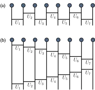
To apply the time-evolution operator we first use the Suzuki-Trotter decomposition to break e−iH(t)τ into a product of local operators. The first order Suzuki-Trotter decompo-sition is
e−iHτ = e−iHoddτe−iHevenτ +O(τ2)
= e−i(H1+H3+···)τe−i(H2+H4+···)τ +O(τ2) (2.33) where H1, H2,· · · are the local Hamiltonians acting on the 1st-2nd sites, 2nd-3rd sites, ...,
as shown in Fig. 2.5. If there are one-site terms in the Hamiltonian, they can be grouped to either side of the two local Hamiltonians as long as the choice is consistent throughout the whole chain. As the local Hamiltonians with the same parity index commute with each other (H1 commutes with H3, H2 commutes with H4, etc. ) Eq. (2.33) can be further
written as
e−iHτ = e−iH1τe−iH3τ· · ·e−iH2τe−iH4τ· · ·+O(τ2)
≡ U1U3· · ·U2U4· · ·+O(τ2) (2.34)
The local time-evolution operators Uk can be easily evaluated. To apply them on the
wave function we need to transform the wave function from the “two-block” setup as in Eq. (2.24) to a “four-block” setup as illustrated in Fig. 2.6, combining the relations of Eq. (2.23) into the new basis the wave function is
|ψi= X
s,n1,n2,e
ψs,n1,n2,e|si|n1i|n2i|ei. (2.35)
H1
H2
H3
H4
H5
H6
H7
2.3 Time-dependent DMRG 17
system
n
1
n
2
environment
1
n
1
n
2
Figure 2.6: Illustration of the four-block setup of the super block basis. The super block wave function is transformed from the original two-block setup used in iDMRG and fDMRG into this four-block setup so that one can apply local operators easily. White’s original version of DMRG [105, 103] also adopted the four-block setup to save memory usage.
Indeed in White’s original version of DMRG [105, 103] he used the four-block setup for iDMRG and fDMRG too because it is more memory efficient than the two-block setup I used. Nowadays the PC memory is several orders of magnitude larger than those when DMRG was first invented in the early 90s, and the bottle neck is no longer the memory but how fast one can compute H|ψi. In the two-block setup the wave function is always stored as a matrix which make it much easier to use some highly optimized linear algebra libraries (MKL, ATLAS) to speed up the H|ψi calculation.
The local time-evolution operator is represented in the local basis |n1i|n2i. Therefore after we transformed the wave function into the four-block setup,U is applied on the wave function as
|ψ0i = U|ψi
= X
n0
1n02n1n1,s,e
Un1n2,n01n02ψs,n01,n02,e|si|n1i|n2i|ei (2.36)
Next we need to shift the basis two sites to the left (right). The procedure is similar to fDMRG except we do not need to calculate the ground state of the super block Hamiltonian. Instead we base on|ψ0ito evaluate the reduced density matrix of the left (right) block and find the renormalization transformation matrices AS (AE) as in Eq. (2.29). This basis shifting technique is called “wave function prediction” by Steven White [106] because it was first used as a guess of the next step wave function in fDMRG to speed up convergence (the speed up is significant therefore should always be used). In this way one can apply all the even bond U during a sweep from left to right, and then all the odd bond U when sweeping back to the left side as illustrated in Fig. 2.7(a). This finishes one time step
τ. Unlike previous time-dependent DMRG where a basis to incorporate wave functions of all time steps is required, t-DMRG always updates the basis to adapt to the current wave function. This saves lots of resources and is the reason behind the name “adaptive time-dependent DMRG”.
In my program I used second order Trotter-Suzuki decomposition, as it is a simple modification to the first order decomposition but has a smaller decomposition error [85, 108].
U
1U
2U
3U
4U
5U
6U
7U
1U
2U
3U
4
U
5U
6U
7
U
7U
6U
5U
4U
3U
2U
1Figure 2.7: Illustration of the application of time-evolution operator decomposed on the wave function. Local time-evolution operators closer to the lattice are applied first. (a) The first order Trotter-Suzuki decomposition; (b) the second order Trotter-Suzuki decom-position. Note that definition of the local time-evolution operators are different in (a) and (b).
whereA andB are non-commute operators. If we letA=H1 andB =H2+H3 +· · · and
use Eq. 2.37 iteratively in this manner we will have
e−iHτ = e−iτ2H1e−iτ2H2· · ·e−iτ2HLe−iτ2HL· · ·e−iτ2H2e−iτ2H1 +O(τ3)
≡ U1U2· · ·ULUL· · ·U2U1+O(τ3) (2.38)
Note here the local time-evolving operators are defined differently as in the second order. They are half time-step operators because one needs to apply them twice to evolve one time step. The application of one time-step τ evolution operator with the second order decomposition on the wave function is illustrated in Fig. 2.7(b). That is when we sweep from left to right we apply U1 to UL one by one, then we sweep back and apply all the
localU operators in the opposite order.
2.4
VMPS
reformulation of density matrix renormalization group method in matrix product state representation [57, 38, 69]. VMPS and DMRG are mathematically equivalent, however VMPS is more concise and easier to deal with both theoretically and numerically. In this thesis, I use VMPS instead of the original DMRG method to study the spin-boson model in Chap. 4.
2.4.1
Matrix product state
The basis transformation of NRG (Eq. (2.22)) and DMRG (Eq. (2.25)) are of the same form, except that we form the transformationAmatrix with different criteria. It is straight-forward to verify that by iteratively using Eq. (2.22) or Eq. (2.25) we can write the wave function in the following form
|ψi=X {nk}
X
α,β,γ,···,µ,ν
A1αn1A2αβn2A3βγn3· · ·ALµνn−1L
−1A
L
νnL|n1, n2, n3,· · · , nL−1, nLi. (2.39)
The coefficients of the wave function are products of matrices, therefore this is called a matrix product state (MPS). MPS is the common mathematical structure underlying NRG and DMRG, therefore it connects the seemingly quite independent methods. MPS enables us to bring some NRG techniques to DMRG and to use DMRG to study open quantum systems [100, 74]. This will be explained in detail in later chapters. In this section, I will only review some general properties of MPS.
If the dimension of the A matrices D is large enough, we can represent any state in MPS form. However, in practice the reason why we want to represent a quantum wave function in the MPS form is that MPS can represent certain kinds of quantum states either exactly or to a very good approximation with relatively small D (D . 100 for example in this thesis). The criteria for such kind of quantum states is that the entanglement of the state is relatively small. Fortunately, this is the case for ground states of 1D quantum lattices due to the area law [69, 24]. However, for excited states when dealing with real-time evolution in true out-of equilibrium, entanglement also can grow, such that t-DMRG is sometimes limited to relatively short time windows.
We can use von Neumann entropy as a measure of the entanglement between two blocks of the whole system. The von Neumann entropy is defined as
S=−T rρlnρ=−X
r
ηrlnηr, (2.40)
with ρ the reduced density matrix and ηr its eigenvalues satisfying P
rηr = 1. Therefore
von Neumann entropy will reach its maximum value when allηr are equal. If we calculate
the reduced density matrix from MPS, the dimension ofρis the same as for theAmatrices. The upper bound for the block entropy is thus
Smax =− D X
r=1
1
Dln
1
Eq. (2.41) implies that the amount of entanglement along the MPS can increase only logarithmically with the matrix dimension D.
An MPS as in Eq. (2.39) contains lots of indices, and thus is a complex representation of a simple many-body wave function. Therefore, it is sometimes more convenient to illustrate the underlying structure pictorially with a diagram like the one shown in Fig. 2.8.
α
β
γ
δ
n
1n
2n
3n
4n
5A
1A
2A
3A
4A
5Figure 2.8: Schematic diagram of a MPS wave function with 5 sites. Squares represent the A-tensors of the MPS, and lines represent their indices. Lines connecting two squares are contracted indices (that is they are summed over). Open lines connect to the basis, and in this diagram they connect to the local basis nk.
Now I will use the 5 sites MPS to show how to calculate (1) an overlap, (2) the action of an operator, and (3) the expectation value with MPS with the help of the schematic diagram. The overlap of two wave functions is calculated by contracting the corresponding local indices of the two wave functions
hψB|ψAi = X
{n0k}
X
α0,β0,γ0,δ0
(Bα10n01B 2 α0β0n02B
3 β0γ0n03B
4 γ0δ0n04B
5 δ0n05)
∗
hn01, n02, n03, n04, n05|
×X
{nk}
X
α,β,γ,δ
A1αn1A2αβn2A3βγn3A4γδn4A5δn5|n1, n2, n3, n4, n5i
= X
{nk}
X
α,β,γ,δ X
α0,β0,γ0,δ0
(Bα10n1B
2 α0β0n2B
3 β0γ0n3B
4 γ0δ0n4B
5 δ0n5)
∗
A1αn1A2αβn2Aβγn3 3A4γδn4A5δn5.
The corresponding diagram for overlap is shown in Fig. 2.9
α
β
γ
δ
n
1n2
n3
n4
n5
A
1A
2A
3A
4A
5B
∗1
α
B
2∗β
B
3∗γ
B
4∗δ
B
5∗Figure 2.9: Schematic diagram of the overlap of two MPS wave functions|ψAi and|ψBi. Complex conjugate tensors will be used when the local indices are pointing up like the B
In DMRG if one wants to apply a local operator on a wave function, one typically needs to perform a partial DMRG sweep to the location where the operator acts. In MPS representation the application of the operator is straight forward since the wave function is expressed in the native local basis. For example the application of a two site operator
U23≡
X
(n0
2n03),(n2n3)
U(n0
2n03),(n2n3)|n 0
2, n
0
3ihn2, n3| (2.42)
is
U23|ψi = X
{nk}
X
α,β,γ,δ
A1αn1A2αβn2A3βγn3A4γδn4A5δn5|n1, n2, n3, n4, n5i
= X
{nk}
X
α,β,δ
A1αn1 X n02,n03,γ,
(U(n2n3),(n02n03)A
2 αβn02A
3 βγn03)A
4 γδn4A
5
δn5|n1, n2, n3, n4, n5i
= X
{nk}
X
α,β,δ
A1αn1Cαγn23 2n3A4γδn4A5δn5|n1, n2, n3, n4, n5i.
Immediately after the operation, this results in the enlarged tensorC23
αγn2n3. To restore the original MPS form, we need to perform singular value decomposition (SVD) on the tensor
Cαγn23 2n3
Cαγn23 2n3 = C(αn23 2),(γn3)
= X
β
˜ ˜
A2(αn2)βλβA˜3β(γn3)
= X
β
˜
A2(αn2)βA˜3β(γn3)
= X
β
˜
A2αβn2A˜3βγn3. (2.43)
In the first line of Eq. (2.43) we reorder and combine the indices of tensorC23and transform
it to a matrix. λβ in the second line is the singular value vector and it is absorbed into
˜
A2
(αn2)β in the third line. In the last line indices are resorted to their MPS order. Fig. 2.10 illustrates this process with a schematic diagram.
The calculation of an expectation value can be reduced to the combination of the previous two operations. However an alternative way is to directly contract all indices. This way also enables us to easily calculate the expectation value of a operator acting simultaneously on any number of sites like the example shown in Fig. 2.11.
2.4.2
Variational matrix product state
α
β
γ
δ
n
1n
4n
5A
1A
2A
3A
4A
5U
23α
γ
δ
n
1n
2n
3n
4n
5A
1C
23A
4A
5n
2n
3α
β
γ
δ
n
1n
4n
5A
1A
˜
2A
˜
3A
4A
5apply local operator
SVD
Figure 2.10: Schematic diagram of applying a local operatorU23on a MPS. First contract the local indices on site 2 and 3 with the indices of U23. This will result a big tensor C23. Then a singular value decomposition is performed to restore the original MPS structure. [See Eq. (2.43)]
VMPS, which means we optimize two sites each time of the optimization. Here we introduce the single site VMPS, which only optimizes one site at each optimization step. Compared with two-site VMPS, it converges slower but the dimension of the optimization problem is smaller than two site VMPS. This is a big advantage when dealing with bosonic systems. Simply speaking VMPS minimizes the energy by variationally optimizing theAmatrices sequentially at a time. At the center of the VMPS calculation is the optimization problem at one site. All the subsystem operators and Hamiltonians are transformed into the effective basis of the current site. The wave function in the local basis is just the A matrix
|ψi= X
αβnk
Akαβnk|α, β, nki. (2.44)
global operator
Figure 2.11: Schematic diagram of calculating the expectation value of a global operator by simply contracting all local indices with the corresponding indices of the global operator. I omit all the labels for simplicity.
problem is transformed into an eigenvalue problem. Similar to DMRG, H is a big sparse matrix, and we cannot and do not have to explicitly expand it into full matrix form. To solve the eigenvalue problem, all we need is to provide the sparse diagonalization algorithm the function |φi=H|ψi. In the |α, β, nki basis the Hamiltonian reads
H = HL⊗Ik⊗IR+IL⊗Ik⊗HR+IL⊗Hk⊗IR
+OL⊗Ok⊗IR+IL⊗Ok⊗OR, (2.45)
with HL andHR the Hamiltonian of the block on the left and right side of the current site k respectively. IL, IR, Ik are identity matrices in their respective spaces. In Eq. (2.45), Hk is the single site term in the Hamiltonian that acts on site k. For example, in the Hamiltonian Eq. (2.18), this is the onsite potential kb
†
kbk. OL and OR are operators on
site k−1 and k + 1 in left and right block basis. Ok is site operator on site k. The last
two terms in the Hamiltonian (2.45) normally consist of several such terms summed over. For simplicity, only a single term is shown. Furthermore, it is assumed throughout that the Hamiltonian is short ranged in that it only contains local and nearest-neighbor terms. Take the Hamiltonian (2.18) for example, with the current site the last two terms in the Hamiltonian (2.45) account for the following four terms: tk−1b
†
k−1bk, tk−1b
†
kbk−1, tkb
†
kbk+1
and tkb
†
k+1bk. Therefore H|ψi can be split into five parts which are illustrated using the
schematic diagram in Fig. (2.12).
Ok and Hk are local operators that act within the Fock space of site k. Their matrix
representations thus are elementary and known from the setup. However the calculation of the block operators and Hamiltonians OL, HL, etc. requires more effort. Let us first
take a close look of the operator OR for example. In the |α, β, nki basis it is OR =
X
β,β0
ORββ0|βihβ0|. (2.46)
Actually OR is just the local operator of site k+ 1 Ok+1 =
X
nk+1,n0k+1
Ok+1n
k+1,n0k+1|nk+1ihn 0
α
β
n
kHL
α
ψ
α
n
kβ
Hk
ψ
nk
α
β
n
k+OL
Ok
ψ
α
n k
α
β
n
kHR
ψ
β
α
β
n
kOR
Ok
ψ
nk
β
+
+
+
=
H
|
ψ
Figure 2.12: Schematic diagram of the five terms in Eq. (2.45) required to computeH|ψi.
and is transformed into the |βibasis according to the basis transformation
|βi= X
γ,nk+1
Ak+1βγn
k+1|γ, nk+1i. (2.48)
The Ak+1βγn
k+1 in this formula is in its “right orthogonal” form which means
X
γ,nk+1
(Ak+1β0γnk+1) ∗
Ak+1βγn
k+1 =δβ0β (2.49)
Any matrixAkin MPS (except the leftmost one) can be right-orthonormalized by a singular
value decomposition. The resulting right matrix from SVD is used as the new Ak and the
left matrix and singular values are absorbed into Ak−1. “Left-orthonormalized”Ak can be calculated in the same way.
Successively applying such basis transformation as Eq. (2.48) we can represent |βiwith the only local basis and the transformation of Ok+1 toOR is illustrated in Fig. 2.13(a). If
the MPS is in its canonical form, that is all matrices have been right-orthonormalized, then (a) reduces to (b). Therefore the calculation of the matrix elements Ok+1 simply requires
ORββ0 =
X
γ,n0
k+1,nk+1 (Ak+1βγn0
k+1) ∗
Onk+1
k+1n0k+1A
k+1
β0γnk+1. (2.50)
The block Hamiltonians HL and HR are calculated iteratively. I take HR (at site k) for
example, and the iterative relation is
HR=Ik+1⊗HR0 +Hk+1⊗IR0 +Ok+1⊗O0R (2.51)
where HR0 is the HR at site k + 1, same for IR0 and O0R. The formula is illustrated in Fig. 2.14. OR0 is obtained in the same way as shown in Fig. 2.13. HR is evaluated using
Eq. (2.51) iteratively from the rightmost site, where HR0 and O0R are both 0. All the HR
and OR at each site are stored for later use.
β
β
Ok+1
O
Rβ
β
Ok+1
O
R(a)
(b)
Figure 2.13: Transforming the local operator into the right block basis. The whole structure inside the dashed line isOR. Because all matrices shown in this plot are assumed to be right-orthonormalized (a) can be reduced to (b).
β
β
β
β
β
β
Hk+1
H
R Ok+1
O
RFigure 2.14: The three terms inHR.
1. Generate a random MPS as the starting point.
2. From the right side calculate HR and OR at each site and store them for later steps.
At the same time the MPS is right-orthonormalized.
3. Optimize the A matrices sequentially at a time from the left side. At the same time calculate and store HL and OL at each site.
4. Repeat step 2 and 3 until convergence is reached. Note that I do not optimize the A
matrices while sweeping from right to left because I only study the Wilson chain in this thesis. Considering the energy scale decreases from left to right, in the spirit of NRG the optimization should start from the high energy end.
5. Calculate physical quantities or flow diagram.
Chapter 3
Landau-Zener problem
3.1
The standard Landau-Zener problem
The standard Landau-Zener problem [50, 117] is a simple time-dependent problem of a two level system. As a highly idealized model it can be used to describe numerous dynamical processes in different contexts like molecular collisions [16], nano-systems [87, 102, 77], Bose-Einstein condensates [112] and quantum information processing [6, 39, 65, 82]. The time-dependent Hamiltonian is
H(t) =
vt
2 ∆
∆ −vt2
, (3.1)
with t the time, v the speed of level crossing and ∆ is the coupling matrix element. For convenience I assume that the two level system consists of a spin. Using Pauli matrices, the Hamiltonian (3.1) becomes
H(t) = vt 2σz+
∆
2σx. (3.2)
At t=−∞ the system is assumed to be in spin up state | ↑i. If v is slow enough so that we can consider the LZ process as an adiabatic process then at t = +∞ the system will still be in the | ↑i state. Beyond the adiabatic limit, there will be some probability for the spin to flip especially around t = 0 when the energy splitting is small. Therefore, at
t= +∞the spin state will be a superposition of| ↓i and| ↑i. The exact calculation of the transition probability is not trivial, but the result is very simple:
P = exp(−π∆
2
2v ). (3.3)
Density matrix renormalization group study of a quantum impurity model with Landau-Zener time-dependent Hamiltonian
Cheng Guo,1,2Andreas Weichselbaum,1Stefan Kehrein,1Tao Xiang,3,2and Jan von Delft1
1Physics Department, Arnold Sommerfeld Center for Theoretical Physics, D-80333 München, Germany
and Center for NanoScience, Ludwig-Maximilians-Universität München, D-80333 München, Germany
2Institute of Theoretical Physics, Chinese Academy of Sciences, P.O. Box 2735, Beijing 100080, China 3Institute of Physics, Chinese Academy of Sciences, P.O. Box 603, Beijing 100080, China
共Received 17 November 2008; revised manuscript received 3 February 2009; published 30 March 2009兲
We use the adaptive time-dependent density matrix renormalization group method共t-DMRG兲to study the nonequilibrium dynamics of a benchmark quantum impurity system which has a time-dependent Hamiltonian. This model is a resonant-level model, obtained by a mapping from a certain Ohmic spin-boson model describ-ing the dissipative Landau-Zener transition. We map the resonant-level model onto a Wilson chain, then calculate the time-dependent occupationnd共t兲of the resonant level. We compare t-DMRG results with exact
results at zero temperature and find very good agreement. We also give a physical interpretation of the numerical results.
DOI:10.1103/PhysRevB.79.115137 PACS number共s兲: 03.65.Yz, 74.50.⫹r, 33.80.Be, 73.21.La
I. INTRODUCTION
Quantum impurity models, describing a discrete degree of freedom coupled to a continuous bath of excitations, arise in many different contexts in condensed-matter physics. In par-ticular, they are relevant for the description of transport through quantum dots and of qubits coupled to a dissipative environment.1,2 In recent years, there has been increasing
interest in studying the real-time dynamics of such models for HamiltoniansH共t兲that are explicitly time dependent, as relevant, for example, to describe external manipulations be-ing performed on a qubit. It is thus important to develop reliable numerical tools that are able to deal with such prob-lems under very general conditions.
The most widely used numerical method to study quan-tum impurity systems is Wilson’s numerical renormalization group 共NRG兲.3 With the recently proposed time-dependent
NRG共TD-NRG兲 共Ref.4兲one can now calculate certain class of time-dependent problems where a sudden perturbation is applied to the impurity at timet= 0. TD-NRG may very well be accurate for arbitrary long time. However, up to now, TD-NRG is not capable of dealing with a Hamiltonian H共t兲
with a time dependence more general than a single abrupt change in model parameters at t= 0. We will show in this paper that the adaptive time-dependent density matrix renor-malization group method共t-DMRG兲is a promising candidate for treating a general time-dependent HamiltonianH共t兲.
The density matrix renormalization group 共DMRG兲 method is traditionally a numerical method to study the low lying states of one-dimensional quantum systems.5 The
re-cent extension of this method, the adaptive t-DMRG,6,7 can
simulate real-time dynamics of one-dimensional models with time-dependent Hamiltonians as well. t-DMRG has already been used to study problems involving real-time dynamics of one-dimensional quantum systems, for example the far-from-equilibrium states in spin-1/2 chains,8dynamics of ultracold
bosons in an optical lattice,9,10 transport through quantum
dots,11dynamics of quantum phase transition,12and
demon-stration of spin charge separation.13These works showed that
t-DMRG is a versatile and powerful method to study the real-time dynamics of one-dimensional quantum systems.
The underlying mathematical structures of DMRG and NRG are similar in the matrix product state representation language.14Indeed, once a quantum impurity model has been
transformed into the form of a Wilson-chain model, it can be treated by DMRG instead of NRG.14–17 This possibility
opens the door toward studying time-dependent quantum im-purity models using t-DMRG. In this paper, we take a first step in this direction by using t-DMRG to study a simple, exactly solvable quantum impurity model whose Hamil-tonian is a function of time. This model allows us to bench-mark the performance of t-DMRG by comparing its results to those of the exact solution.
II. MODEL AND DMRG METHOD
We study the resonant-level model with a time-dependent potential applied to the level. The Hamiltonian is
Hˆ共t兲=⑀d共t兲d†d+
兺
k⑀kck
†
ck+V
兺
k共d†ck+ck
†
d兲. 共1兲
d† creates a spinless fermion on the level共impurity兲andc
k
† creates a spinless fermion with momentumkin a conduction band whose density of states is constant between −DandD
and zero otherwise, with Fermi energy set equal to 0. The energy of the local band is swept linearly with time,
⑀d共t兲=Dvt, where vis the sweeping rate in units of the half
band width D. This model is equivalent to the dissipative Landau-Zener model with a Ohmic boson bath whose spec-tral function isJ共兲= 2␣, forⰆc, wherecis the high
energy cutoff,18and the dimensionless strength of dissipation
parameter␣is henceforth set equal to12. When␣is close but not equal to 12, Hamiltonian共1兲contains an additional inter-action term proportional to U共d†d−12兲共兺k,k⬘ck
†
ck⬘− 1
2兲,
19 but
this case will not be considered here.
At timet0→−⬁the local level contains a spinless fermion and the band is half filled. Then, we lift the energy of the