www.geosci-model-dev.net/7/495/2014/ doi:10.5194/gmd-7-495-2014
© Author(s) 2014. CC Attribution 3.0 License.
Geoscientific
Model Development
Improving predictive power of physically based rainfall-induced
shallow landslide models: a probabilistic approach
S. Raia1, M. Alvioli1, M. Rossi1, R. L. Baum2, J. W. Godt2, and F. Guzzetti1
1CNR IRPI, via Madonna Alta 126, 06128 Perugia, Italy
2US Geological Survey, P.O. Box 25046, Mail Stop 966, Denver, CO 80225-0046, USA
Correspondence to: M. Alvioli ([email protected])
Received: 7 January 2013 – Published in Geosci. Model Dev. Discuss.: 21 February 2013 Revised: 29 January 2014 – Accepted: 13 February 2014 – Published: 25 March 2014
Abstract. Distributed models to forecast the spatial and temporal occurrence of rainfall-induced shallow landslides are based on deterministic laws. These models extend spa-tially the static stability models adopted in geotechnical en-gineering, and adopt an infinite-slope geometry to balance the resisting and the driving forces acting on the sliding mass. An infiltration model is used to determine how rain-fall changes pore-water conditions, modulating the local sta-bility/instability conditions. A problem with the operation of the existing models lays in the difficulty in obtaining accurate values for the several variables that describe the material properties of the slopes. The problem is partic-ularly severe when the models are applied over large ar-eas, for which sufficient information on the geotechnical and hydrological conditions of the slopes is not generally available. To help solve the problem, we propose a prob-abilistic Monte Carlo approach to the distributed modeling of rainfall-induced shallow landslides. For this purpose, we have modified the transient rainfall infiltration and grid-based regional slope-stability analysis (TRIGRS) code. The new code (TRIGRS-P) adopts a probabilistic approach to com-pute, on a cell-by-cell basis, transient pore-pressure changes and related changes in the factor of safety due to rainfall in-filtration. Infiltration is modeled using analytical solutions of partial differential equations describing one-dimensional vertical flow in isotropic, homogeneous materials. Both sat-urated and unsatsat-urated soil conditions can be considered. TRIGRS-P copes with the natural variability inherent to the mechanical and hydrological properties of the slope materi-als by allowing values of the TRIGRS model input param-eters to be sampled randomly from a given probability dis-tribution. The range of variation and the mean value of the
parameters can be determined by the usual methods used for preparing the TRIGRS input parameters. The outputs of sev-eral model runs obtained varying the input parameters are an-alyzed statistically, and compared to the original (determinis-tic) model output. The comparison suggests an improvement of the predictive power of the model of about 10 % and 16 % in two small test areas, that is, the Frontignano (Italy) and the Mukilteo (USA) areas. We discuss the computational re-quirements of TRIGRS-P to determine the potential use of the numerical model to forecast the spatial and temporal oc-currence of rainfall-induced shallow landslides in very large areas, extending for several hundreds or thousands of square kilometers. Parallel execution of the code using a simple pro-cess distribution and the message passing interface (MPI) on multi-processor machines was successful, opening the possi-bly of testing the use of TRIGRS-P for the operational focasting of rainfall-induced shallow landslides over large re-gions.
1 Introduction
1998; Baum et al., 2002, 2008, 2010; Crosta and Frattini, 2003; Simoni et al., 2008; Godt et al., 2008; Vieira et al., 2010) approaches, or a combination of them (Gorsevski et al., 2006; Frattini et al., 2009). Inspection of the liter-ature, reveals that process-based (deterministic, physically based) models are preferred to forecast the spatial and the temporal occurrence of shallow landslides triggered by indi-vidual rainfall events in a given area. Process-based mod-els rely upon the understanding of the physical laws con-trolling slope instability. Due to lack of information and the poor understanding of the physical laws controlling landslide initiation, only simplified, conceptual models currently are possible. These models extend spatially the simplified stabil-ity models widely adopted in geotechnical engineering (e.g., Taylor, 1948; Wu and Sidle, 1995; Wyllie and Mah, 2004), and calculate the stability/instability of a slope using param-eters such as normal stress, angle of internal friction, co-hesion, pore-water pressure, root strength, seismic acceler-ation, or external weights. Computation results in the factor of safety, an index expressing the ratio between the local re-sisting (R) and driving (S) forces,FS=R/S. Values of the
index smaller than 1, corresponding toR < S, denote insta-bility, on a cell-by-cell basis, according to the adopted model. To calculate the resisting and the driving forces, the geome-try of the sliding mass must be defined, including the geom-etry of the topographic surface and the location of the slip surface. Most commonly, an infinite-slope approximation is adopted (Taylor, 1948; Wu and Sidle, 1995). This is also the approach adopted by the US Geological Survey (USGS) Transient Rainfall Induced and Grid-Based Regional Slope-Stability Model (TRIGRS) model (Baum et al., 2002, 2008), within each user-defined cell. Within the infinite-slope ap-proximation, in each cell the slip surface is assumed to be of infinite extent, planar, at a fixed depth, and parallel to the topographic surface. Forces acting on the sides of the sliding mass are neglected.
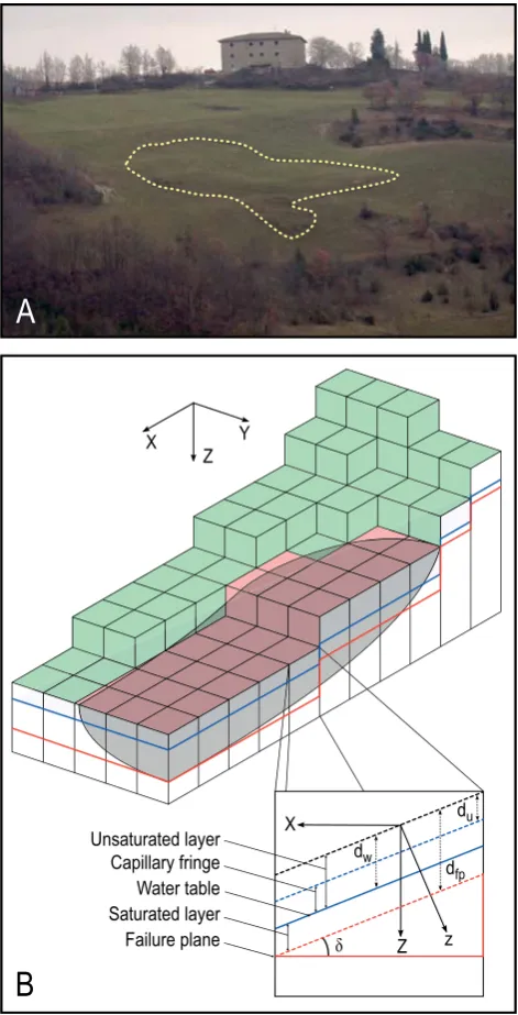
Modeling of shallow landslides (Fig. 1a) triggered by rainfall adopting the infinite-slope approach requires time-invariant and time-dependent information. Time-time-invariant in-formation includes the mechanical and hydrological proper-ties of the slope material (e.g., unit weightγ, cohesionc, angle of internal frictionφ, water content θ, saturated hy-draulic conductivityKs), and the geometrical characteristics of the sliding mass (e.g., gradient of the slope and the sliding planeδ, depth to the sliding planedfp). The fact that these pa-rameters are constant in time is an assumption of the model. Time-dependent information consists of the pressure headψ, that is, the pressure exerted by water on the sliding mass, which is a function of the depth,dw of water in the terrain
(Freeze and Cherry, 1979). Determining the pressure head, and its spatial and temporal variations, requires understand-ing how rainfall infiltrates and water moves into the ground. This is described by the Richards equation (Richards, 1931). This non-linear partial differential equation does not have a closed-form analytical solution, and approximate solutions
Capillary fringe Unsaturated layer
Water table Saturated layer Failure plane
X
Z
δ z
du
dw
dfp
X Z
Y
A
B
Fig. 1. (A) Example of a rainfall-induced shallow landslide of
the soil slide type in the Collazzone area, Umbria, Italy (Fig. 7).
(B) Schematic representation of the slope-infinite model showing
the coordinate system and variables used in the deterministic and probabilistic models. See Table A1 for the symbols description.
are used for saturated (e.g., Iverson, 2000) and unsaturated (e.g., Srivastava and Yeh, 1991; Savage et al., 2003, 2004) conditions.
saturated conditions. In the code, the forces acting on each individual grid cell are balanced in the centre of mass of each cell, and all interactions with the neighboring grid cells are neglected.
In a second release of TRIGRS, Baum et al. (2008) have extended the code to include unsaturated soil conditions, including the presence of a capillary fringe above the wa-ter table. TRIGRS can be used for modeling and forecast-ing the timforecast-ing and spatial distribution of shallow, rainfall-induced landslides in a given area (Baum et al., 2002, 2008, 2010). A problem when using TRIGRS, and similar com-puter codes (e.g. Shalstab, Montgomery and Dietrich, 1994; GEOtop-SF, Simoni et al., 2008), for the modeling of shallow rainfall-induced landslides over large areas resides in the dif-ficulty (or operational impossibility) of obtaining sufficient, spatially distributed information on the mechanical and hy-drological properties of the terrain. Adoption of a particular value to describe the mechanical (unit weightγs, cohesionc, angle of internal frictionφ) and the hydrological (water con-tentθ, saturated hydraulic conductivityKs) properties of the
terrain may result in unrealistic or inappropriate representa-tions of the stability condirepresenta-tions of individual or multiple grid cells.
In this work, we propose a probabilistic, Monte Carlo ap-proach in an attempt to overcome the problem of poor knowl-edge of terrain characteristics over large study areas. We ob-tain the input values for the parameters for the individual runs of TRIGRS using probability distributions. Multiple simu-lations are performed with different sets of randomly cho-sen input parameters, and we obtain multiple sets of model outputs. We denote the newly developed code TRIGRS-Probabilistic, or TRIGRS-P. The different outputs are then analysed jointly to infer local stability or instability con-ditions as a function of the random variability of the in-put parameters, and the statistical significance of the mul-tiple outputs is determined. Examples of similar probabilis-tic approaches to model the stability/instability conditions of slopes exists in the literature (e.g., Hammond et al., 1992; Pack et al., 1998; Haneberg, 2004). The various models adopt different physically based models, which are not equivalent. We maintain that the probabilistic approach of the modified version of TRIGRS is relevant, because it considers most of the aspects relevant to slope stability analysis, and it is ca-pable of reproducing empirical properties of rainfall-induced shallow landslides, including the rainfall intensity–duration conditions that generate the slope instabilities, and the statis-tics of the size of the unstable areas, as recently shown by Alvioli et al. (2014).
The paper is organized as follows. First, we summarize the model adopted in the software code TRIGRS, version 2.0 (Baum et al., 2008), and we introduce our probabilistic extension (Sect. 2) implemented in the new code TRIGRS-P. Next, we present a comparison of the performance of the original and the probabilistic simulations for two study areas: Mukilteo, USA, and Frontignano, Italy (Sect. 3). Results are
discussed in Sect. 4, which focuses on the analysis of the performance of the geographical prediction of the shallow landslides, and on the potential application of the new proba-bilistic code for modeling shallow rainfall-induced landslides over large areas (>100 km2).
2 Overview of the model
Both TRIGRS and TRIGRS-P frameworks are pixel-based and adopt the same geometrical scheme, the same subdivi-sion of the geographical domain and accept the same inputs. An additional set of parameters is used in TRIGRS-P to spec-ify the variability of the characteristics of the terrain. Within each pixel, slopes are modeled as a two-layer system consist-ing of a lower saturated zone with a capillary frconsist-inge above the water table, overlain by an unsaturated zone that extends to the ground surface. The water table and the (hypotheti-cal) sliding surface are planar and parallel to the topographic surface. The geographical domain represented by an array of grid cells, coincides with the elements of a digital elevation model (DEM) used to describe the topography of the study area (Fig. 1b).
2.1 Deterministic approach: the TRIGRS code
In the original approach coded in TRIGRS (Baum et al., 2008), the stability of an individual grid cell is determined adopting the one-dimensional infinite-slope model Taylor (1948). The model assumes that failure of a grid cell occurs when the resisting forcesRacting on the sliding surface are less than the driving forcesS (Wu and Sidle, 1995; Wyllie and Mah, 2004). The ratio of the resistingRand the driving
Sforces gives by the factor of safetyFS,
FS=
R
S =
tanφ
tanδ +
c−ψ γwtanφ
γszsinδcosδ , (1)
where the internal friction angleφ, the cohesionc, and the soil unit weightγsdescribe the material properties,γwis the groundwater unit weight,δ is the angle of the planar slope, andψ is the pressure head (Fig. 1b, see Table A1). Failure occurs when FS<1. Solution of Eq. (1) requires the
com-putation of the pressure headψ, which is governed by the Richards (1931) equation:
∂ ∂z
Kz(ψ )∂ (ψ−z)
∂z
=∂θ
∂t , (2)
wherezis the slope-normal coordinate,t is the time,Kzis
the vertical hydraulic conductivity that depends on the pres-sure headψ, andθis the volumetric water content (Fig. 1b). Equation (2) is solved in TRIGRS adopting the modeling scheme proposed by Baum et al. (2008).
Again, the modification consists chiefly in the possibility of using a complex rainfall history (Baum et al., 2008). To lin-earize Eq. (2), Iverson (2000) adopted a normalization crite-rion using a length scale ratio as follows:
ε=
s
dfp2/D0
A/D0
=√dfp
A, (3)
whereD0is the maximum hydraulic diffusivity,Ais the
con-tributing area that affects hydraulic pressure at the potential failure plane depthdfp, anddfp2/D0andA/D0are the
mini-mum time required for slope-normal (dfp2/D0) and for
slope-lateral (A/D0) pore-pressure transmission (see Table A1).
Under the conditionε1, simplification of Eq. (2) gives (Iverson, 2000)
∂
∂z∗
K∗(ψ )
∂ψ∗
∂z∗ −z
∗
=0, for t > A
D0 (4)
and
∂
∂z∗
K∗
∂ψ∗
∂z∗ −z
∗
=C(ψ )
C0
∂ψ∗
∂t∗ , for t
A
D0, (5)
whereψ∗=ψ/dfp,t∗=t D/A, andz∗=z/p
dfp.
For unsaturated conditions, the code uses a modified version of the analytical solution of Eq. (2) proposed by Srivastava and Yeh (1991), for the case of one-dimensional, transient, vertical infiltration. The modification consists in the use of a variable rainfall history (intensity, duration), allowing modeling of complex rainfall patterns (Baum et al., 2008). Equation (2) was linearized in Srivastava and Yeh (1991), who adopted the following exponential model (Gardner, 1958):
Kz(ψ )=Kseαψe; (6)
θ=θr+(θs−θr) eαeψ, (7)
whereKs is the saturated hydraulic conductivity, θr is the
residual water content,θsis the saturated water content, and e
ψ=ψ−ψ0, ψ0= −1/α is a constant, withα the inverse
of the vertical height of the capillary fringe above the water table (Savage et al., 2003, 2004). Substitution of Eq. (7) into Eq. (2) leads to the partial differential equation:
α (θs−θr)
Ks ∂K
∂t =
∂2K
∂z2 −α
∂K
∂z . (8)
Equation (8) is a linear diffusion equation for which analyti-cal solutions can be obtained using the Laplace, the Fourier, or the Green’s function methods (Kevorkian, 1991), once boundary conditions are specified, for example,
K(z,0)=IZLT−IZLT−Kseαψ0e−αz; (9)
K(0, t )=Kseαψ0, (10)
whereIZLTis the steady surface flux, which can be approx-imated by the average precipitation rate necessary to main-tain the initial conditions in the days to months preceding an event (Baum et al., 2010). When a solution of Eq. (8) is obtained, the pore-pressure headψcan be calculated by in-version of Eq. (2). Solutions of Eq. (8) with the boundary conditions listed in Eq. (10) are given in Appendix A1.
TRIGRS implements a simple surface runoff routing scheme to disperse the excess water from the grid cells where rainfall intensity exceeds the local infiltration capacity (Hillel, 1982; Baum et al., 2008).
2.2 Probabilistic approach: the TRIGRS-P code
In our extension of the TRIGRS code, we use the same model and equations as in the original code. The innovation consists of using probability distributions to model the slope material and hydrological properties, that is, the values of the input parameters. The geometry of the slope (δ) and the position of the sliding plane (dfp) remain unchanged. The model
pa-rameters appearing in the equations described in Sect. 2.1 are replaced by functions of random numbers, that is,
c=c(ξc),cohesion;
φ=φ (ξφ),angle of internal friction;
γs=γ (ξγ),soil unit weight;
D0=D0(ξD0),hydraulic diffusivity;
Ks=Ks(ξKs),saturated hydraulic conductivity; θr=θr(ξθr),residual water content;
θs=θs(ξθs),saturated water content;
α=α(ξα),inverse height of capillary fringe, (11)
whereξi is a random number, with the subscript i used to
specify a different parameter,ξcfor cohesion,ξφfor friction,
etc., so that the parameters can be varied independently from each other. Replacing the parameters listed in Eq. (11) into Eqs. (1), (2), (4), (5), and (8), we obtain a system of equa-tions that are initialized with a different, randomly chosen set of parameters at each run of TRIGRS-P. The solution of the various scenarios for saturated or unsaturated conditions are performed in the very same way as in TRIGRS. The depth to the potential sliding planedfp was assumed to coincide with the soil depth, and was estimated by Godt et al. (2008) and Baum et al. (2010) using variations of the models proposed by DeRose (1996) and by Salciarini et al. (2006). Additional choices for initial conditions and corresponding sources of uncertainties will be discussed in the following.
We have implemented two probability density functions (pdf) for generating the modeling parameters: (i) the nor-mal distribution function N, and (ii) the uniform distri-bution function U. If ξ is a standard normally distributed variable N(0,1) with mean ξ¯=0 and standard deviation
σ=1, the variablex=x+σxξ is normally distributed with
is standard uniformly distributed U(0,1), the variable y= ya+(yb−ya)ξis uniformly distributed in the range[ya, yb],
U(ya, yb). The advantage of using these expansions is that
their deterministic limits are obtained for σx→0 and for
λ≡yb−ya→0.
In this work, we calculated the stability conditions in the modeling domain for a given set of variables describing the slope materials properties (φ,c,γs,Ks,D0,θr,θs) obtained
by sampling randomly from the uniform distribution only. There is a conceptual difference between the two distribu-tions for distributed landslide probabilistic modeling. Adop-tion of the Gaussian distribuAdop-tion requires that the investiga-tor has determined (e.g., through sufficient field tests or lab-oratory experiments) the uncertainty and measuring errors associated with the parameters. The mean and the standard deviation of the Gaussian distribution define unambiguously the uncertainty. Use of the uniform distribution implies that the investigator only knows the possible (or probable) range of variation of the parameters, ignoring the internal struc-ture of the uncertainty. We consider the Gaussian distribu-tion more appropriate to predict rainfall-induced landslides in small areas where sufficient field and laboratory tests were performed to characterize the physical properties of the ge-ological materials, and the uniform distribution best suited in the investigation of large areas where information on the geo-hydrological properties is limited. Further, we consider use of the Gaussian distribution best suited to investigate how errors in the parameters propagate and affect the modeling re-sults, provided that the errors are known. Conversely, use of the uniform distribution allows for investigating how the un-certainty in the model parameters affects the model results. The sensitivity of the extended model to the random varia-tion of model parameters has been explored by running 16 independent simulations, each with a different set of input parameters while keeping unchanged, and equal to the run performed with the original fixed-input TRIGRS model, the terrain morphology (δ) and rainfall history.
3 Deterministic vs. probabilistic approach
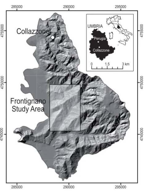
We tested the performance of the new probabilistic version of the numerical code, TRIGRS-P 2.0, against the original TRIGRS code, version 2.0 (Baum et al., 2008), in two study areas. The first test was conducted in the Mukilteo study area, near Seattle, WA, USA (Fig. 2). This is the same geograph-ical area where Godt et al. (2008) and Baum et al. (2010) demonstrated the use of TRIGRS in a broad geographical setting. The second test was performed in the Frontignano study area, Perugia, Italy (Fig. 7). This is part of the Col-lazzone geographical area where Guzzetti et al. (2006a, b) have investigated the hazard posed by shallow landslides us-ing multivariate classification methods.
Fig. 2. The location of the Mukilteo study area, near Seattle, WA,
USA.
3.1 Mukilteo study area
The three square kilometer study area is located along the eastern side of the Puget Sound, about 15 km north of Seattle, WA, USA (Fig. 2). In this area, rainfall is the primary trig-ger of landslides. Slope failures are typically shallow (less than three meters thick), and involve the sandy colluvium and the weathered glacial deposits mantling the coastal bluffs (Galster and Laprade, 1991; Baum et al., 2000). The cli-mate of the Seattle area is characterized by a pronounced seasonal precipitation regime with a winter maximum, and three-fourths of the annual precipitation falling from Novem-ber to April (Church, 1974). Storms that trigger shallow land-slides in Seattle are generally of long duration (more than 24 h) and of moderate intensity (Godt et al., 2006). Three ge-ological units crop out in the area (Minard, 2000) (Fig. 3a) in-cluding, from older to younger: (i) transition sediments, com-prising the Lawton Clay (Qtb); (ii) advance outwash sand (Qva); and (iii) glacial till (Qvt). The mechanical and hy-drological properties of the materials in the three geologi-cal units are known through field tests and laboratory experi-ments (Lu et al., 2006; Godt et al., 2006, 2008), and are sum-marized in Table 1.
3.1.1 Predictions with the deterministic approach
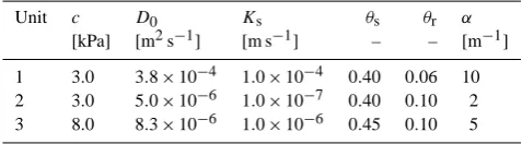
Table 1. Geotechnical parameters for the geological units cropping
out in the Mukilteo area (Fig. 3a).c: cohesion;D0: hydraulic
dif-fusivity;Ks: saturated hydraulic conductivity;θs: saturated water
content;θr: residual water content; α: inverse of capillary fringe. The friction angleφhas a common value of 33.6◦for the three ge-ological units; units definitions are 1: Qtb; 2: Qva; 3: Qvt.
Unit c D0 Ks θs θr α
[kPa] [m2s−1] [m s−1] – – [m−1]
1 3.0 3.8×10⁻⁴ 1.0×10⁻⁴ 0.40 0.06 10 2 3.0 5.0×10⁻⁶ 1.0×10⁻⁷ 0.40 0.10 2 3 8.0 8.3×10⁻⁶ 1.0×10⁻⁶ 0.45 0.10 5
through airborne laser-swath mapping (Haugerud et al., 2003). Initial conditions for infiltration were prescribed as zero pressure head at the depth of the lower boundary of col-luvium. This is in agreement with field observations (Baum et al., 2005; Schulz, 2007; Godt et al., 2008). A constant rainfall intensity I =4.5 mm h−1 for a period of 28 h was used to force slope instability, for a cumulative event rainfall
E=126 mm. The adopted rainfall history represents a lim-ited case of the rainfall intensity–duration conditions that have resulted in landslides in the Mukilteo area in the winter 1996–1997 (Godt et al., 2008; Baum et al., 2010). Figure 3 shows the results of the runs with deterministic input, for sat-urated (Eq. 4, Fig. 3b) and for unsatsat-urated (Eq. 5, Fig. 3c) conditions. For the mechanical and hydrological properties of the geological materials (φ,c,γs,Ks,D0,θr,θs) we con-sidered the values listed in Table 1.
In order to test the model prediction skills, that is, the ability of the model to forecast the known distribution of rainfall-induced landslides (Guzzetti et al., 2006a), the two geographical distributions of the factor of safety FS were
compared to a landslide inventory showing slope failures triggered by rainfall in the winter 1996–1997 (Baum et al., 2000; Godt et al., 2008), displayed by black lines in Fig. 3. For the comparison, all grid cells withFS<1 were
consid-ered unstable (i.e., potential landslide) cells. Fourfold plots and maps showing the geographical distribution of the cor-rect assignments and the model errors (Fig. 3e, f) are used to summarize and display the comparison. Fourfold plots are graphical representations of contingency tables (or confusion matrices), and show the fraction (or number) of true posi-tives (TP), true negaposi-tives (TN), false posiposi-tives (FP), and false negatives (FN) (Fawcett, 2006; Rossi et al., 2010). In our analysis TP is the percentage of cells with observed land-slides, which are predicted as unstable by the model; simi-larly, TN is the percentage of cells without landslides pre-dicted as stable by the model. Correspondingly, FP (FN) are the percentage of predicted unstable (stable) cells with-out (with) observed landslides. We will refer to both TP and TN as correct assignment in the following, while FP and FN are model errors. To further quantify the perfor-mance of the deterministic forecasts, different metrics were
1278000 1280000
344000
346000
340000
342000
343000
345000
339000
341000
1277000 1279000 A
1278000 1280000
344000
346000
340000
342000
343000
345000
339000
341000
1277000 1279000 B
1278000 1280000
343000
345000
339000
341000
343000
345000
339000
341000
1277000 1279000 C
Qvt Qva Qtb
1278000 1280000
344000
346000
340000
342000
343000
345000
339000
341000
1277000 1279000 D
1278000 1280000
344000
346000
340000
342000
343000
345000
339000
341000
1277000 1279000 E
1278000 1280000
344000
346000
340000
342000
343000
345000
339000
341000
1277000 1279000 F
0°
90° 79.5
6.0 10.4
4.1
TP FP TN FN
56.1
3.0 33.8
7.1
TP FP TN FN
Factor of safety, Fs ≤ 0.7 (0.7, 0.8] (0.8, 0.9] (0.9, 1.0] (1.0, 1.1] (1.1, 1.2] (1.2, 1.3] (1.3, 1.4] (1.4, 1.5] > 1.5
Factor of safety, Fs ≤ 0.7 (0.7, 0.8] (0.8, 0.9] (0.9, 1.0] (1.0, 1.1] (1.1, 1.2] (1.2, 1.3] (1.3, 1.4] (1.4, 1.5] > 1.5
Fig. 3. Mukilteo study area; results obtained using the original
TRI-GRS code and input parameters of Table 1. (A) Lithology map: Qtb, transition sediments, including the Lawton Clay (1 in Table 1); Qva, advance outwash sand (2 in Table 1); Qvt, glacial till (3 in Table 1).
(B) Factor of safety FS obtained with saturated soil conditions;
(C)FSobtained with unsaturated soil conditions; (D) slope map; (E) map of correct assignments and model errors, within the
satu-rated model; TP: True Positive; TN: True Negative; FP: False Pos-itive; FN: False Negative; (F) as in (E), for the unsaturated model. Black polygons show rainfall-induced landslides.
computed (Table 2), including the true positive rate (sensitiv-ity, or hit rate) TPR=TP/(TP+FN), the true negative rate (specificity) TNR=TN/(FP+TN), the false positive rate (1 – specificity, or false alarm rate) FPR=FP/(FP+TN), the accuracy ACC=(TP+TN)/(TP+FN+FP+TN), and the precision PPV=TP/(TP+FP)(Fawcett, 2006; Baum et al., 2010).
3.1.2 Predictions with the probabilistic approach
Based on the comparison of the results discussed in the pre-vious section, for the probabilistic modeling we used only the unsaturated soil conditions, and we exploited the same geomorphological information (i.e., the same DEM) and the same rainfall forcing input (i.e., 4.5 mm h−1of rain for a 28 h period) used for the previous runs. For the mechanical and hydrological properties of the geological materials (φ,c,γs, Ks,D0,θr,θs), we considered the values listed in Table 1,
Table 2. Estimators of model performance for saturated and
unsat-urated soil calculated with the original TRIGRS code, for the Muk-ilteo study area. TPR: true positive rate; FPR: false positive rate; ACC: accuracy; PPV: precision.
Model type TPR FPR ACC PPV
Saturated 0.71 0.38 0.63 0.17 Unsaturated 0.41 0.12 0.84 0.28
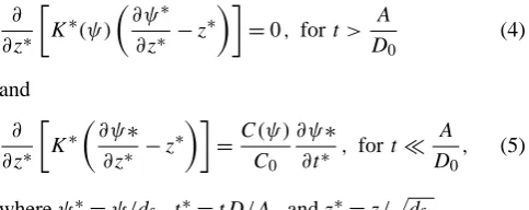
as mean values of uniformly distributed variablesU(ya, yb), whereya andybare the lower and upper limits of the uni-form distribution determining the range of variation of each parameter. In our simulations, the range of variation of the individual parameters has been chosen as a fraction of the mean value of each variable. A range of variationλ=0.01, 0.10 and 1.00 correspond to a variation of 1 %, 10 % and 100 % around the mean value of the variable, respectively. Note that the case withλ=0.01 allows the various input pa-rameters to vary in a very limited range, and it can be seen as a test of our code: the original TRIGRS results with fixed input parameters should be obtained.
We performed two sets of runs. In the first set, the mean values of the mechanical and hydrological parameters (Ta-ble 1) were kept constant, and the range of variation of the individual parameters was modulated using λ=0.01, 0.1, 0.5, 1.0. In the second set, a fixed range of variation for the individual parameters was selected,λ=1.0, and the mean value of the parameters was modified (shifted) byν=0.2,
0.4, . . . ,1.0, 2.0. Note that whenν=1.0, no shift of the mean
value is performed. In each test, the same range of varia-tionλand the same shift of the mean valueνwere applied to all the parameters. The simplification was adopted to re-duce the time required to perform multiple runs. The results are shown in Fig. 4: (i) for the first set of runs, that is, for fixed mean values of the model parameters and changing ranges of variation of the individual parameters, λ=0.01 (Fig. 4a),λ=0.5 (Fig. 4b), and λ=1.0 (Fig. 4c); and (ii) for the second set of runs, that is, for a fixed range of vari-ationλ=1.0, and shifting the mean value of the model pa-rameters byν=0.8 (Fig. 4d),ν=0.9 (Fig. 4e), andν=1.1 (Fig. 4e). For the second set of runs, results obtained for
ν <0.8 and forν >1.1 are not shown in Fig. 4. Forν <0.8
the number of unconditionally unstable cells was unrealisti-cally large, and forν >1.1 the model performance decreased rapidly (see next paragraph). We used 16 runs for each set, resulting in 16 different maps of the factor of safety, which were used to evaluate the performance of the probabilistic approach. The results are shown in Fig. 5. For the same runs of Fig. 4, the maps show the geographical distribution of the correct assignments (TP, TN), the model errors (FP, FN), and the corresponding fourfold plots. Tables 3 and 4 list metrics that quantify the performance of the probabilistic approach.
1278000 1280000
344000
346000
340000
342000
343000
345000
339000
341000
1277000 1279000 B
1278000 1280000
343000
345000
339000
341000
343000
345000
339000
341000
1277000 1279000 C
1278000 1280000
344000
346000
340000
342000
343000
345000
339000
341000
1277000 1279000 A
1278000 1280000
344000
346000
340000
342000
343000
345000
339000
341000
1277000 1279000 E
1278000 1280000
343000
345000
339000
341000
343000
345000
339000
341000
1277000 1279000 F
1278000 1280000
344000
346000
340000
342000
343000
345000
339000
341000
1277000 1279000 D
λ=0.01
ν=0.8
λ=0.5 λ=1.0
ν=1.1
ν=0.9
0.7 0.8 0.9 1.0 1.1 1.2 1.3 1.4 1.5 Factor of safety, Fs
Fig. 4. Mukilteo study area. Maps showing factor of safetyFS
ob-tained with the code presented in this work, TRIGRS-P, initialized with the same input parameters used for the same area and TRIGRS code, in Fig. 3, and with the following parameters for the random number generation: (A) λ=0.01,ν=1.0; (B) λ=0.5, ν=1.0;
(C)λ=1.0,ν=1.0. (D)λ=0.5,ν=0.8; (E)λ=0.5,ν=0.9;
(F)λ=0.5,ν=1.1. We performed 16 runs for each set of param-eters. Black polygons show rainfall-induced landslides; the insets show the spatial variability of the factor of safety.
3.1.3 Analysis and discussion
Table 3. Estimators of model performance of the results obtained
with the TRIGRS-P code in the Mukilteo study area. In this case we change the ranges of variation of the model parametersλ, with fixed mean values of the model parametersν=1.0. TPR: true positive rate; FPR: false positive rate; ACC: accuracy; PPV: precision; AUC: area under the ROC curve.
λ TPR FPR ACC PPV AUC
0.01 0.41 0.11 0.84 0.29 0.65 0.10 0.41 0.11 0.84 0.29 0.70 0.50 0.40 0.12 0.83 0.28 0.73 0.75 0.34 0.11 0.83 0.26 0.71 1.00 0.09 0.04 0.87 0.22 0.67
Table 4. As in Table 3, but with fixed ranges of variation of the
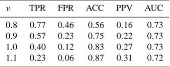
model parametersλ, and with varying the mean values of the model parameters, for the Mukilteo area.
ν TPR FPR ACC PPV AUC
0.8 0.77 0.46 0.56 0.16 0.73 0.9 0.57 0.23 0.75 0.22 0.73 1.0 0.40 0.12 0.83 0.27 0.73 1.1 0.23 0.06 0.87 0.31 0.72
and of Table 2 indicates that the model prepared consider-ing the soil unsaturated conditions (Fig. 3c) performed bet-ter than the model prepared considering saturated conditions (Fig. 3b). The larger value of the TPR/FPR ratio is a mea-sure of the better predicting performance of the unsaturated model (TPR/FPR=3.46, Fig. 6), compared to the saturated model (TPR/FPR=1.87, Fig. 3), despite a lower TPR value (TPR=0.42 vs. TPR=0.71, Table 2). This is in agreement with previous work of Godt et al. (2008) and Baum et al. (2010).
Within the two deterministic models, the one using the un-saturated soil conditions (Fig. 3c, f) performed better than the model that used the saturated soil conditions (Fig. 3b, e). The saturated model predicted a significantly larger fraction of the study area as unstable, mainly where the terrain gradient exceeded 15◦. This resulted in a considerably larger number of true positives (TP: 7.1 % vs. 4.1 %), but also a significantly larger number of false positives (FP: 33.8 % vs. 10.4 %) and a correspondingly significantly lower number of true nega-tives (TN: 56.1 % vs. 79.5 %). In other words, the saturated deterministic model (Fig. 3b) was more pessimistic than the unsaturated deterministic model (Fig. 3c). This is well rep-resented in Fig. 6, where a reduction of the false positive rate from 0.38 to 0.12 results in a reduction of the hit rate from 0.71 to 0.41 (Table 2). The subsequent runs with proba-bilistic input were obtained assuming unsaturated soil water conditions. The results of the unsaturated probabilistic mod-els (Fig. 4) were similar to the results of the corresponding
1278000 1280000
344000
346000
340000
342000
343000
345000
339000
341000
1277000 1279000 B 1278000 1280000
344000
346000
340000
342000
343000
345000
339000
341000
1277000 1279000 A
1278000 1280000
344000
346000
340000
342000
343000
345000
339000
341000
1277000 1279000 C 1278000 1280000
344000
346000
340000
342000
343000
345000
339000
341000
1277000 1279000 E 1278000 1280000
344000
346000
340000
342000
343000
345000
339000
341000
1277000 1279000 D
1278000 1280000
344000
346000
340000
342000
343000
345000
339000
341000
1277000 1279000 F λ=0.01
ν=0.8
λ=0.5 λ=1.0
ν=1.1 ν=0.9
79.5
6.0 10.4
4.1
TP FP TN FN
49.0
2.4 40.9
7.7
TP FP TN FN
69.2
4.4 20.7
5.7
TP FP TN FN
84.9
7.8 5.0
2.3
TP FP TN
FN
79.4
6.0 10.5
4.1
TP FP TN FN
79.3
6.1 10.6
4.0
TP FP TN
FN
Fig. 5. Maps of correct assignments and model errors in the
Mukil-teo study area, obtained with the TRIGRS-P code with different sets of random input parameters. (A) λ=0.01,ν=1.0; (B)λ=0.5,
ν=1.0; (C)λ=1.0,ν=1.0. (D)λ=0.5, ν=0.8; (E)λ=0.5,
ν=0.9; (F)λ=0.5,ν=1.1. TP: true positive; TN: true negative; FP: false positive; FN: false negative. In all maps, black polygons show rainfall-induced landslides in the study area.
unsaturated deterministic model (Fig. 3c). This is a signif-icant result, confirming that treating the uncertainty asso-ciated with the model parameters with a probabilistic ap-proach has not significantly changed the model results, which have remained consistent. Availability of multiple model out-puts for each run allowed preparing ROC curves to measure quantitatively the predictive performance of the probabilis-tic models (Fawcett, 2006). Since multiple values ofFS are available for each pixel in the modeling domain, we can cal-culate the frequency of stability condition of each pixel. We attribute to this frequency the meaning of a probability and compare it with a given threshold. Modulation of the classi-fication threshold allows us to obtain different FPR and TPR values, which can be used to construct a ROC curve (Fawcett, 2006). In Fig. 6 two sets of ROC curves are shown using different colors. The red curves show the performances of the first set of runs, forλ=0.01,λ=0.5, andλ=1.0, with
ν=1.0, and the blue curves show the performances of the second set of runs, forν=0.8, ν=0.9, andν=1.1, with
0.0 0.2 0.4 0.6 0.8 1.0
0.0
0
.2
0.4
0
.6
0.8
1
.0
False Alarm Rate
Hit Rate
AUC AUC
0.1 0.65 0.8 0.73 0.5 0.73 0.9 0.73 1.0 0.67 1.1 0.72 Variable range Variable mean
ν (λ=0.5)
λ
Probabilistic runs Deterministic unsaturated
Deterministic saturated
Fig. 6. The results of simulations for the Mukilteo study area,
pre-sented using ROC curves. The grey square and circle represent the results obtained using the original TRIGRS code with saturated and unsaturated initial conditions, respectively (Fig. 3b, c); the curves correspond to the results obtained with the TRIGRS-P code, using the variability of input parameters shown in the inset as described in the text (Figs. 4 and 5).
under the ROC curve AUC is taken as a quantitative mea-sure of the performance of the classification. If AUC=0.5, a classification is poor and indistinguishable from a random classification, whereas a perfect classification has AUC=1 (Fawcett, 2006; Rossi et al., 2010).
Inspection of Figs. 5 and 6, and of Table 3, suggests that an increase in the range of variation of the model param-eters (fromλ=0.01 toλ=1.0), corresponding to a signifi-cantly larger degree of uncertainty in the parameters, resulted in similar individual performance indices, but significantly larger values of the area under the ROC curve, AUC. In our experiment, the increase in the range of variation changed the performance index from AUC=0.65 (forλ=0.01) to AUC=0.73 (forλ=0.5), with an increase of performance of 16 %. A further increase of the range of variation toλ=
1.0, a possibly unrealistic range of variation for some of the modeling parameters, has resulted in a value of AUC=0.67, decreasing the model performance. Modulation of the mean value of the parameters, usingν=0.8,ν=0.9, andν=1.1, resulted in better results (larger AUC values) forλ=0.5 than forλ=0.01. Moreover, the TPR, FPR, PPV and ACC met-rics did not change significantly when the range of variation
λof the model parameters were modified, and remained sim-ilar to the values obtained with the deterministic models, for
λ≤0.5. We conclude that, in the Mukilteo study area, these metrics are not sensitive to introduction of the probabilis-tic determination of the model parameters. Second, the AUC
285000 290000
4755000
4745000
295000
285000 290000 295000
4755000
4745000
4750000 4750000
0 1.5 3 km
Collazzone UMBRIA
Frontignano
Study Area
Collazzone
Perugia
Fig. 7. Map showing location of the Frontignano study area,
Um-bria, central Italy. The area is located inside the larger Collazzone area (Guzzetti et al., 2006a, b).
showed a positive correlation with the range of variation in the model parameters.
In the probabilistic runs, a positive correlation was ob-served between the range of variationλand the fraction of unconditionally unstable cells, that is, the grid cells that have
FS<1 even in dry conditions when no rainfall is increasing
pore-pressure and slope instability. For the first set of runs, the fraction of unconditionally unstable cells was 0 % for
λ=0.01, 0.3 % forλ=0.5, and 0.7 % forλ=1.0. More-over, a negative correlation was observed between ν, the width of shift in the mean value of the modeling parame-ters, and the fraction of unconditionally unstable cells. For the second set of runs, the fraction of unconditionally unsta-ble cells was less than 5.0 % forν≥0.8, and was 0 % for
ν >1.0, independent of the range of variation of the
param-eters.
3.2 Frontignano study area
288500 289500
4748500
4749500
4745500
4746500
4747500
4748000
4749000
4746000
4747000
290500
289000 290000 291000
288500 289500
4748500
4749500
4745500
4746500
4747500
4748000
4749000
4746000
4747000
290500
289000 290000 291000 288500 289500
4748500
4749500
4745500
4746500
4747500
4748000
4749000
4746000
4747000
290500
289000 290000 291000
Factor of safety, Fs 0.7 0.9 1.1 1.3 1.5
0° Slope, δ 90° flysch
sdLithologycl gr-sd-st-cl sd-st-cl
A B C
288500 289500
4748500
4749500
4745500
4746500
4747500
4748000
4749000
4746000
4747000
290500
289000 290000 291000
D
288500 289500
4748500
4749500
4745500
4746500
4747500
4748000
4749000
4746000
4747000
289000 290000 291000 290500
E
289500
4748500
4749500
4745500
4746500
4747500
4748000
4749000
4746000
4747000
290500
289000 290000 291000 288500
F
74.1
0.9 24.4
0.6 TP
FP
TN
FN
85.8
1.2 12.7
0.3
TP FP
TN
FN
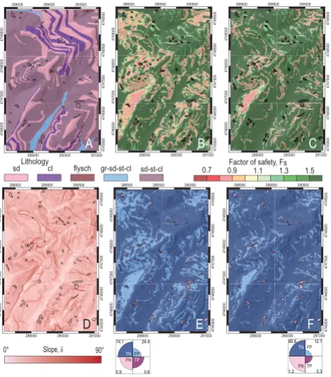
Fig. 8. As in Fig. 3, but for the Frontignano study area. The results
have been obtained using the original TRIGRS code with input pa-rameters listed in Table 5. (A) Lithological map: sand (1 in Table 5); clay (2 in Table 5); flysch deposits (3 in Table 5); gravel, sand, silt, and clay (4 in Table 5); sand, silt, and clay (5 in Table 5). (B) Factor of safetyFS obtained with saturated soil conditions; (C)FS
ob-tained with unsaturated soil conditions; (D) slope map; (E) map of correct assignments and model errors, within the saturated model; TP: true positive; TN: true negative; FP: false positive; FN: false negative; (F) as in (E), for the unsaturated model. Black polygons show rainfall-induced landslides.
slides were identified in the area through the visual interpre-tation of multiple sets of aerial photographs and very-high resolution satellite images, and field surveys.
The shallow failures are typically less than three meters thick, and involve the soil and the colluvium mantling the slopes. Soils range in thickness from a few decimeters to more than one meter; they have a fine to medium texture, and exhibit a xeric moisture regime, typical of the Mediterranean climate. In central Umbria, precipitation is most abundant in October and November, with a mean annual rainfall in the period 1921–2001 exceeding 850 mm. In the study area, ter-rain is hilly, and the lithology and the altitude of bedding planes control the morphology of the slopes. Gravel, sand, clay, travertine, layered sandstone and marl, and thinly lay-ered limestone crop out in the area (Cardinali et al., 2000; Guzzetti et al., 2006a, b).
3.2.1 Predictions with the deterministic approach
For modeling purposes, the topography of the Frontignano study area was described by a 5 m×5 m DEM obtained in-terpolating 5 m contour lines shown on 1:10 000 scale to-pographic base maps (Guzzetti et al., 2006a, b). Slope in the area ranges from 0◦to 62◦, with an average value of 10◦and a standard deviation of 5.6◦ (Fig. 8d). The mechanical and hydrological properties of the five soil types cropping out in the area (Fig. 8a) were determined through laboratory tests and searching the literature (see, e.g. Shafiee, 2008; Feda et al., 1995; Lade, 2010, and references therein) on the geotech-nical properties (φ,c,γs,Ks,D0,θr,θs) of the same or sim-ilar sediments in Umbria, Italy (listed in Table 5). As for the Mukilteo area, the depth to the hypothetical sliding planedfp
was assumed to coincide with the soil depth, which was esti-mated using the model proposed by DeRose (1996). To cal-ibrate the soil depth model, we exploited field observations indicating that the depth of the shallow landslides in the study area isdfp<3 m, and that shallow landslides are most
abun-dant where terrain gradient is in the range 7◦≤δ≤20◦. Ini-tial depth to the water table was set to a fraction of the depth to the failure plane,dw=0.85dfp. Since the depth of the
wa-ter table is an important initial condition for the model, we decided to use a long rainfall period, starting from an almost dry initial condition and reaching a realistic depth of the wa-ter table during the storm. We further decided not to set the water table to the maximum soil depth to consider the fact that the simulation is intended to be representative of typical winter conditions, when landslides occur in both study areas, and when the soil always contains some amount of water. We tested different rainfall histories, and adopted a forcing rain-fall that produced shallow landslides in the area in the periods January–May 2004, October–December 2004, and October– December 2005 (Guzzetti et al., 2009; Fiorucci et al., 2011). Specifically, we used a rainfall history composed of a 4-week initial rainfall period characterized by a constant mean rainfall intensityI=0.36 mm h−1, for a cumulative rainfall
E=242 mm, followed by a 60 min rainfall period character-ized by a high rainfall intensityI=90 mm h−1, for a cumu-lative rainfallE=90 mm. Results for the saturated (Eq. 4) and the unsaturated (Eq. 5) modeling conditions are shown in Fig. 8b and c, respectively.
To test the model performance, the geographical distribu-tion of the factor of safety FS predicted by TRIGRS were compared to the known distribution of rainfall-induced land-slides mapped in the same area in the periods January to May 2004, October to December 2004, and October to De-cember 2005. The landslides were mapped through recon-naissance fieldwork and the visual interpretation of high-resolution satellite images (Guzzetti et al., 2009; Fiorucci et al., 2011), and are shown with black lines in Fig. 8. For the comparison, all grid cells withFS<1 were considered
Table 5. Geotechnical parameters for the geological units cropping
out in the Frontignano study area (Fig. 8a).c: cohesion;φ: friction angle;D0: hydraulic diffusivity;KS: saturated hydraulic
conductiv-ity;θs: saturated water content;θr: residual water content;α: inverse of capillary fringe. Geological units: 1: sand; 2: clay; 3: flysch de-posits; 4: gravel, sand, silt, and clay; 5: sand, silt, and clay.
Unit c φ D0 Ks θs θr α
[kPa] [deg] [m2s−1] [m s−1] – – [m−1]
1 3.0 31 3.8×10⁻⁴ 1.0×10⁻⁴ 0.20 0.05 2
2 4.0 18 5.0×10⁻⁶ 1.0×10⁻⁷ 0.80 0.07 5
3 50.0 25 8.3×10⁻⁶ 1.0×10⁻⁶ 0.45 0.1 5
4 15.0 30 4.0×10⁻⁴ 1.0×10⁻⁴ 0.45 0.1 5
5 3.0 15 4.7×10⁻³ 1.0×10⁻⁴ 0.50 0.1 1
Table 6. As in Table 2, but for the Frontignano area.
Model type TPR FPR ACC PPV
Saturated 0.42 0.25 0.75 0.02 Unsaturated 0.18 0.13 0.86 0.02
ROC plots (Fig. 11), and maps showing the geographical distribution of the correct assignments and the model errors (Fig. 8e, f) were used to summarize and measure the compar-ison.
Inspection of Figs. 8 and 11, and analysis of Table 6, sug-gests that the saturated and the unsaturated models produce very similar results. This is different from the result obtained in the Mukilteo area, where the unsaturated model performed better than the saturated model. In the Frontignano area, the unsaturated model (Fig. 8c) resulted in a better forecasting accuracy (ACC, 0.86 vs. 0.75), but in a reduced TPR to FPR ratio (1.4 vs. 1.7). We maintain that the model prepared con-sidering the saturated conditions (Fig. 8b) performed slightly better than the model obtained considering the unsaturated conditions (Fig. 8c).
3.2.2 Predictions with the probabilistic approach
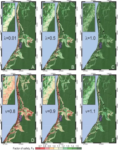
The mechanical and hydrological properties of the geological materials (φ,c,γs,Ks,D0,θr,θs) in the Frontignano study area were chosen as listed in Table 5 (also used as input of the original TRIGRS model, in the previous paragraph) as mean values of uniformly distributed variablesU(ya, yb). To be consistent with the approach adopted in Mukilteo, we per-formed two sets of parametric analyses, varying the range (λ) and the mean value (ν) of the model parameters. The maps in Fig. 9 show the factor of safetyFScalculated for (i) fixed
mean values of the model parametersν=1.0, and chang-ing ranges of variation of the individual parameters,λ=0.01 (Fig. 9a),λ=0.75 (Fig. 9b), andλ=1.0 (Fig. 9c); and (ii) a fixed range of variationλ=0.75, and shifting the mean value of the model parameters byν=0.8 (Fig. 9d),ν=0.9
288500 289500
4748500
4749500
4745500
4746500
4747500
4748000
4749000
4746000
4747000
290500
289000 290000 291000 288500 289500
4748500
4749500
4745500
4746500
4747500
4748000
4749000
4746000
4747000
290500
289000 290000 291000
288500 289500
4748500
4749500
4745500
4746500
4747500
4748000
4749000
4746000
4747000
289000 290000 291000
290500 289500
4748500
4749500
4745500
4746500
4747500
4748000
4749000
4746000
4747000
290500
289000 290000 291000 288500
288500 289500
4748500
4749500
4745500
4746500
4747500
4748000
4749000
4746000
4747000
290500
289000 290000 291000 288500 289500
4748500
4749500
4745500
4746500
4747500
4748000
4749000
4746000
4747000
290500
289000 290000 291000
Factor of safety, Fs 0.7 0.8 0.9 1.0 1.1 1.2 1.3 1.4 1.5
A B C
D E F
ν=0.8 ν=1.1
λ=0.01 λ=0.75 λ=1.0
ν=0.9
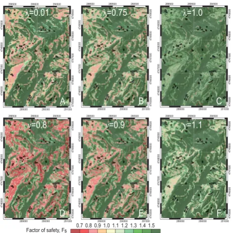
Fig. 9. Frontignano study area. Maps of the factor of safetyFS
ob-tained within the probabilistic approach of TRIGRS-P, with the fol-lowing values of range of variation of input parameters: (A)λ=
0.01,ν=1.0; (B)λ=0.75,ν=1.0; (C)λ=1.0,ν=1.0. (D)λ=
0.75,ν=0.8; (E)λ=0.75,ν=0.9; (D)λ=0.75,ν=1.1. We per-formed 16 runs for each set of parameters. In all maps, black poly-gons show rainfall-induced landslides in the study area.
(Fig. 9e), and ν=1.1 (Fig. 9f). As in the previous case,
λ=0.01 corresponds to a very small range of variability of the parameters, and provides the same results. Forν=1.0, no shift in the mean values of the model parameters is per-formed. The degree of accuracy of the two sets of runs for the Frontignano area is shown in Fig. 10, for the same mod-els shown in Fig. 9. The maps show the geographical distri-bution of the correct assignments (TP, TN), the model errors (FP, FN), and the corresponding fourfold plots. Tables 7 and 8 list metrics that quantify the performance of the runs. The performance of the probabilistic models is further analysed in Fig. 11 by two sets of ROC curves, shown using different colours; red curves for the case of variable rangeλ, and blue curves for the case of a variable meanν. In the same plot, the grey circle shows the predicting performance of the sat-urated model (Fig. 8b), and the grey square the performance of the unsaturated model (Fig. 8c) both run with fixed input parameters.
3.2.3 Analysis and discussion
288500 289500 4748500 4749500 4745500 4746500 4747500 4748000 4749000 4746000 4747000 290500
289000 290000 291000
288500 289500 4748500 4749500 4745500 4746500 4747500 4748000 4749000 4746000 4747000 290500
289000 290000 291000
288500 289500 4748500 4749500 4745500 4746500 4747500 4748000 4749000 4746000 4747000
289000 290000 291000
290500 289500 4748500 4749500 4745500 4746500 4747500 4748000 4749000 4746000 4747000 290500
289000 290000 291000 288500 288500 289500 4748500 4749500 4745500 4746500 4747500 4748000 4749000 4746000 4747000 290500
289000 290000 291000 288500 289500 4748500 4749500 4745500 4746500 4747500 4748000 4749000 4746000 4747000 290500
289000 290000 291000
A B C
D E F
ν=0.8 ν=1.1
λ=0.01 λ=0.75 λ=1.0
ν=0.9 74.5 0.8 27.0 0.7 TP FP TN FN 82.2 1.1 16.3 0.4 TP FP TN FN 94.9 1.4 3.6 0.1 TP FP TN FN 74.1 0.9 24.4 0.6 TP FP TN FN 62.5 0.7 36.0 0.8 TP FP TN FN 92.1 1.3 6.4 0.2 FP TN FN TP
Fig. 10. Frontignano study area. Maps of the factor of correct
as-signments and model error obtained within the probabilistic ap-proach of TRIGRS-P, with the following values of range of variation of input parameters: (A)λ=0.01,ν=1.0; (B)λ=0.75,ν=1.0;
(C)λ=1.0,ν=1.0. (D)λ=0.75,ν=0.8; (E)λ=0.75,ν=0.9;
(D)λ=0.75, ν=1.1. TP: true positive; TN: true negative; FP: false positive; FN: false negative. In all maps, black polygons show rainfall-induced landslides in the study area.
discussed for the Mukilteo study area (see Sect. 3.1.3), with a few differences. In the Frontignano area, the saturated and the unsaturated models provided nearly equivalent results, with the saturated model considered marginally superior pri-marily because of the reduced value of the TPR to FPR ratio. From a statistical point of view, given the reduced fraction of landslide area in Frontignano (1.5 %) compared to Muk-ilteo (4.2 %), the spatial prediction of landslides in Frontig-nano was more difficult than in Mukilteo. From a physical point of view, modeling the stability conditions in low gra-dient terrain is very sensitive to the initial conditions, which are uncertain and difficult to determine spatially. The runs with variable input parameters confirm the slightly poorer geographical predictive performance of the adopted physi-cal framework in Frontignano, compared to Mukilteo (Ta-bles 3 and 4 vs. Ta(Ta-bles 7 and 8). Taking the area under the ROC curve (AUC) as the metric to compare the models, one can readily see that runs for the Mukilteo area resulted in 0.65≤AUC≤0.73, and for the Frontignano area exhibited 0.59≤AUC≤0.65. In other words, the “worst” result for Mukilteo (AUC=0.65, for ν=1.0 and λ=0.01) has the same overall spatial predictive performance of the “best” re-sult for Frontignano (AUC=0.65, for ν=0.8 or 0.9 and
0.0 0.2 0.4 0.6 0.8 1.0
0.0 0 .2 0.4 0 .6 0.8 1 .0
False Alarm Rate
Hit Rate
AUC AUC
0.1 0.59 0.8 0.65 0.75 0.64 0.9 0.64 1.0 0.63 1.1 0.64 Variable range Variable mean
ν (λ=0.75)
λ
Probabilistic runs Deterministic unsaturated
Deterministic saturated
Fig. 11. Frontignano study area; ROC plots corresponding to the
runs with fixed input parameters (Fig. 8b, c) and with the proba-bilistic approach with random input parameters (Figs. 9 and 10).
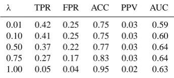
Table 7. As in Table 3, but for the Frontignano area.
λ TPR FPR ACC PPV AUC
0.01 0.42 0.25 0.75 0.03 0.59 0.10 0.41 0.25 0.75 0.03 0.60 0.50 0.37 0.22 0.77 0.03 0.64 0.75 0.27 0.17 0.83 0.03 0.64 1.00 0.05 0.04 0.95 0.02 0.63
λ=0.75). In the Frontignano area, despite a lower “abso-lute” performance (i.e., when compared to Mukilteo), adop-tion of a probabilistic approach improved the spatial fore-casting skills. Again, taking AUC as a metric to compare the models, values of this metric increased from AUC=0.59 (for ν=1.0 and λ=0.01) to AUC=0.65 (for ν=0.8 or 0.9 andλ=0.75). This is a non-negligible improvement of about 10 %. The result confirms that adoption of a probabilis-tic framework to the distributed modeling of shallow land-slides results in improved spatial forecasts.
Table 8. As in Table 4, but for the Frontignano area.
ν TPR FPR ACC PPV AUC
0.8 0.57 0.37 0.63 0.02 0.65 0.9 0.44 0.27 0.72 0.02 0.64 1.0 0.27 0.17 0.83 0.03 0.64 1.1 0.10 0.06 0.92 0.02 0.64
Second, the area under the ROC curve AUC confirmed its positive correlation with the range of variation in the model parametersλ, in support of the probabilistic approach. Third, the positive correlation between the range of variationλand the fraction of unconditionally unstable cells, and the neg-ative correlation between the shift in the mean value of the modeling parametersν and the fraction of unconditionally unstable cells, were both confirmed.
4 Discussion
Our probabilistic approach to the distributed modeling of shallow landslides proved effective in the two study areas where it was tested (Figs. 2 and 7). In both areas, the maps showing the geographical distribution of the factor of safety
FS obtained using TRIGRS-P were better predictors of the distributions of known rainfall-induced landslides than the corresponding maps obtained adopting the original TRIGRS approach. This conclusion is supported by the indices used to measure the forecasting skills of the different models, and particularly the area under the ROC (AUC) (Tables 2–4 for Mukilteo, and Tables 6, 7, 8 for Frontignano). The runs in which we allowed a large variability of the input parameters (e.g.λ=0.50 orλ=0.75) were better predictors of the ge-ographical distribution of known landslides than the models prepared using a reduced variability in the model parameters (e.g.λ=0.1) (Guzzetti et al., 2006a; Rossi et al., 2010). This is shown in the insets in Fig. 4, where a portion of the results for the Mukilteo study area is shown at a larger scale. The variability of the geographical distribution of theFSis also shown in Fig. 12 where we have plotted the minimum, the maximum, and the standard deviation of the computed FS
values. In particular, the map of the standard deviation pro-vides quantitative and spatially distributed evidence of the uncertainty associated with the distributed modeling of land-slide instability.
We studied the variation of the computed factor of safety. Figure 13 shows histograms for the distribution of the val-ues of the factor of safetyFS in selected grid cells in the
Mukilteo (Fig. 13a–c) and the Frontignano (Fig. 13d–f) study areas. For simplicity, in the figure we show the results ob-tained for a single lithological type, that is, the transition sed-iments (Qtb, indicated as unit 1 in Table 1) in the Mukilteo area (Fig. 3a), and the sand–silt–clay (unit 5 in Table 5) in
1278000 1280000
344000
346000
340000
342000
343000
345000
339000
341000
1277000 1279000 B
1278000 1280000
343000
345000
339000
341000
343000
345000
339000
341000
1277000 1279000 C 1278000 1280000
344000
346000
340000
342000
343000
345000
339000
341000
1277000 1279000 A
Factor of safety, Fs 288500 289500
4748500
4749500
4745500
4746500
4747500
4748000
4749000
4746000
4747000
290500
289000 290000 291000
288500 289500
4748500
4749500
4745500
4746500
4747500
4748000
4749000
4746000
4747000
290500
289000 290000 291000 288500 289500
4748500
4749500
4745500
4746500
4747500
4748000
4749000
4746000
4747000
290500
289000 290000 291000
A B C
λ=0.01 λ=0.5 λ=1.0
Std. dev. 0.250.50 0.75 1.00 A
E
B C
D F
0.7 0.8 0.9 1.0 1.1 1.2 1.31.41.5
Fig. 12. Maps showing the minimum (left column), maximum
(cen-ter column), and standard deviation (right column) of the factor of safetyFS for the set of 16 simulation runs using the TRIGRS-P
code. Maps are shown for the Mukilteo (upper row) and the Fron-tignano (lower row) study areas.
the Frontignano area (Fig. 8a). Results for other lithologi-cal types in the two study areas are similar. We adopted the following procedure to obtain the histograms. First, we per-formed 100 probabilistic simulations to obtain a large set of values of the factor of safetyFS, and we computed the
av-erage value of the factor of safety,FS for each grid cell in
the two modeling domains. For both study areas, a value of λ=0.50 (and ν=1.0) was used for the variability of the geotechnical and hydrological parameters. Next, we se-lected three subsets of 1000 grid cells, with 0< FS≤1.5,
1.5< FS≤3.0, andFS>3, respectively. Finally, we used
all the computed values of theFSin each subset to construct the histograms. Inspection of the histograms reveals that for
FS>3 (Fig. 13c, f) the distribution of the predicted factor
of safety is almost uniform and does not show a predomi-nant value. Instead, forFS<1.5 the distribution of the
pre-dicted factors of safety peaks atFS≈1.0 (Fig. 13a, d). For
1.5< FS≤3.0, results are intermediate (Fig. 13b, e).
In conclusion, the probabilistic approach results in a num-ber of model outputs, each representing the geographical dis-tribution of theFS values. In this work, 16 runs were
Count
0
500
1000
1500
2000
2500
Count
0
500
1000
1500
2000
Factor of safety, Fs
Count
0 2 4 6 8 10
0
500
1000
1500
2000
0 1 2 3 4 5 6 7 8 9 10
Count
0
500
1000
1500
2000
2500
Count
0
500
1000
1500
2000
Factor of safety, Fs
Count
0 2 4 6 8 10
0
500
1000
1500
2000
0 1 2 3 4 5 6 7 8 9 10
A
C B
D
E
F
Fig. 13. Histograms showing the distribution of the values of the FS for the Mukilteo (left, A, B, C) and the Frontignano (right, D, E, F) study areas. (A) and (D) for subsets of 1000 grid cells with
0< FS≤1.5. (B) and (E) for subsets of 1000 grid cells with 1.5<
FS≤3. (C) and (F) for subsets of 1000 grid cells withFS>3.
depends on multiple causes (Uchida et al., 2011), including (i) the natural variability in the geotechnical and hydrological properties of the soils, (ii) the inability of determining accu-rate values for the geotechnical and hydrological parameters, and (iii) the fact that the models are simplified and do not represent the natural (physical) conditions in the study area.
The probabilistic approach allowed the investigation of the combined effects of the natural variability inherent in the model parameters, and of the uncertainty associated with their definition over large areas. However, the approach can-not separate the two causes for the variability. Also, the prob-abilistic approach cannot validate the physics in the model better than the deterministic approach. It should be noted that in our runs with probabilistic input parameters, the geotech-nical and hydrological properties were treated explicitly as independent (uncorrelated) variables. This was a simplifica-tion. In reality, some dependence (correlation) exists between the different geo-hydrological properties. As an example, the saturated water contentθsaffects the saturated hydraulic
conductivityKs and the hydraulic diffusivityD0. However,
selection of values for the different properties based on field tests, laboratory experiments, or through a literature search resulted in values for the considered properties that were im-plicitly dependent. This is because, for example, cohesion, angle of internal friction, soil unit weight, and hydraulic con-ductivity depend one upon the other. Furthermore, no spa-tial correlation of the individual variables was considered in the modeling. This was also a simplification, because spa-tial correlation exists between the geo-hydrological proper-ties (e.g., Rodriguez-Iturbe et al., 1999; Western et al., 2004). Adoption of the uniform distribution to determine the possi-ble range of variation of the individual parameters, combined with the accepted modeling simplifications, has resulted in more “extreme” results, but not in unrealistic results.
Results of our approach were obtained adopting the uni-form distribution to describe the uncertainty associated with the geo-hydrological parameters. TRIGRS-P allows for the use of the Gaussian and the uniform distributions. In the runs presented in this work, we explored only part of the variabil-ity associated with the physical model describing slope insta-bility forced by rainfall infiltration (Fig. 1b), and specifically the variability associated with the mechanical and hydrolog-ical parameters of the materials involved in the hypotheti-cal landslides. We did not consider the lohypotheti-cal morphologihypotheti-cal variability, for example, the uncertainty in the description of the terrain given by the DEMs. Terrain gradient is an im-portant parameter for the computation of the factor of safety
FS. Inspection of Eq. (1) shows that variability in the terrain gradientδ results in variability in the local stability condi-tions, measured byFS. Furthermore, in our runs soil depth was a (non-linear) function of the local slope (DeRose, 1996; Salciarini et al., 2006). Variations in the slope will result in variations in soil thickness, and in the local stability condi-tions. Preliminary results obtained adding a uniform random perturbation to the DEM for the Frontignano area confirmed the (large) sensitivity of the physically based models to the topographic information (Montgomery and Dietrich, 1994; van Westen et al., 2008; Tarolli et al., 2012).
different rainfall histories (e.g., (i) a uniform rainfall rate of 0.36 mm h−1 for a 4-week period, for a cumulated rainfall
E=242 mm; (ii) a single rainfall event with 5 mm h−1 for 24 h,E=121 mm; and (iii) intermittent 3-day rainfall peri-ods withI =1.0 mm h−1separated by 4-day dry periods, for a 4-week period,E=288 mm) revealed that the geographi-cal distributions of theFSobtained with the different rainfall
histories were similar. However, the local instability condi-tions (FS≤1) were reached at different times. The difference
may be significant if the model results are used in a landslide early warning system (Aleotti, 2004; Godt et al., 2006). We did not evaluate the sensitivity of the model parameters to the different rainfall histories.
It should be noted that the probabilistic approach of TRIGRS-P could be used to infer reasonable values of the parameters describing terrain characteristics, where they are largely unknown, by exploring a large parameter space in a random way and comparing with known distributions of landslides.
Adoption of a probabilistic approach with multiple runs using a randomly generated different set of input parame-ters results in longer computer processing times. The time required for a single TRIGRS-P simulation is only slightly longer than the time needed for the corresponding TRIGRS simulation, since the random variables were computed be-fore running the slope stability and infiltration model. The time for this initial step depends on the size (in grid cells) and complexity of the modeling domain. The processing time of the multiple runs required by the TRIGRS-P approach to have a statistical significance may be easily reduced by exploiting the multi-core architecture of modern CPUs, just running simultaneously multiple instances of the TRIGRS-P code initialised with different sets of parameters. Since our aim is to eventually use the TRIGRS as a region-wide and possibly nation-wide early warning system, we give an es-timate of the computing resources required. Using the same spatial resolution, a larger area will require a larger process-ing time, with the time increasprocess-ing linearly with the number of grid cells. The time required for a simulation depends also on rainfall history. A more complex history (i.e., a shorter step between two subsequent inputs of rainfall intensity) will re-sult in a longer processing time, with time increasing with the square of the time steps. Finally, processing time de-pends on the type of hydrological model used, with the sat-urated model requiring roughly half the time of the unsatu-rated model.
When using the probabilistic approach, we adopted a strat-egy based on a convergence level,η. First, we computed two probabilistic sets withn and m > n simulations. Next, for the two independent sets and for each grid cell, we com-puted the mean of the factor of safety FS. Then, we
ob-tained the difference of the mean values of the factor of safety
1FS for each cell, and we identified the maximum value of
max(1FS)in the modeling domain. If max(1FS)≤η, the
convergence level was reached and no additional simulations
10-3 105 104 103 102 101
10-2 100 10-1 106 107
10-1 106 105 104 103 102 101 100 107 108
105 104 103 102 101 100
Memory usage [
Gb
]
Area [km2]
Execution time [
s
]
A
TRIGRS - saturated model
1×1 m
30×30 m 10×10 m 5×5 m 2×2 m
10-3 105 104 103 102 101
10-2 100 10-1 106 107
10-1 106 105 104 103 102 101 100 107 108
105 104 103 102 101 100
Memory usage [
Gb
]
Area [km2]
Execution time [
s
]
B
TRIGRS-S - unsaturated model
1×1 m
30×30 m 10×10 m 5×5 m 2×2 m
Fig. 14. Estimated memory usage (leftyaxis) and execution times
(rightyaxis) for (A) the TRIGRS code (saturated model), and (B) a set of 16 runs of the TRIGRS-P code, for areas of different extent, and for grid cells of different spatial resolutions.
were performed. Instead, if max(1FS) > ηconvergence was
not reached, a larger probabilistic set was prepared, and the test repeated. In our two study areas, 16 simulations were sufficient to obtain a convergence levelη=0.05. This level was considered adequate for the two study areas. This may not be the case in other areas, in significantly large areas, or in areas characterized by a larger physiographical variability. For simulations covering large areas, we hypothesized areas extending between 101and 105km2with grids of resolution from 1 m×1 m to 30 m×30 m, and computed the memory usage and execution time for (i) a single deterministic sim-ulation adopting a saturated soil model (Fig. 14a); and (ii) a probabilistic set of 16 simulations using an unsaturated soil model (Fig. 14b).
Since the TRIGRS (and TRIGRS-P) model uses a cell-by-cell description of the study area, and the equations de-scribing the stability of each cell are independent from the neighboring cells behavior, the code is most suited for a par-allel implementation using MPI libraries. We performed pre-liminary simulations, showing that a significant speed-up ('1/N, with N the number of processing elements used) can be obtained for the computing-intensive portions of the code. One problem associated with significantly large areas is the use of memory. In a truly parallel implementation of the code, each computing element or core should load into memory only the portion of data relevant to its task, which is currently not implemented.
5 Conclusions