R E S E A R C H A R T I C L E
Open Access
Sharp bounds on sufficient-cause
interactions under the assumption of no
redundancy
Wen-Chung Lee
Abstract
Background:Sufficient-cause interaction is a type of interaction that has received much attention recently. The sufficient component cause model on which the sufficient-cause interaction is based is however a non-identifiable model. Estimating the interaction parameters from the model is mathematically impossible.
Methods:In this paper, I derive bounding formulae for sufficient-cause interactions under the assumption of no redundancy.
Results:Two real data sets are used to demonstrate the method (R codes provided). The proposed bounds are sharp and sharper than previous bounds.
Conclusions:Sufficient-cause interactions can be quantified by setting bounds on them.
Keywords:Sufficient component cause model, Epidemiologic methods, Causal inference, Interaction, Identifiability
Background
A common aim of many observational studies is to identify risk factors for disease. Once risk factors have been identi-fied, researchers will often be interested in knowing whether any two factors can interact in causing the disease.
‘Sufficient-cause interaction’(also referred to as‘synergism’,
‘causal co-action,’‘causal mechanistic interaction, or simply’
‘mechanistic interaction’) is a type of interaction that has received much attention recently [1–11] and is based on Rothman’s sufficient component cause model [12, 13]. The model posits that the causation of disease can be through any one of many different mechanisms or pathways. A mechanism/pathway requires several different component causes to operate, hence it is also called a‘causal pie’. If two factors participate in the same causal pie, then a sufficient-cause interaction can be said to exist between them.
If the monotonicity assumption is not imposed [14–18], the sufficient component cause model in its general form is over-parameterized and non-identifiable. That is, the total number of model parameters exceeds the total degrees of
freedom the data can offer. For example, two binary risk fac-tors mean the data can offer at most four degrees of freedom (four different exposure profiles) but the model has a total of nine parameters, each corresponding to one of the nine possible causal-pie classes (one ‘all-unknown’ class unre-lated to either factor, two main-effect classes for each factor, and four two-factor interaction classes). [If the monoton-icity assumption is imposed on the two factors, the number of causal-pie classes reduces to four (one‘all-unknown’class unrelated to either factor, one main-effect class for each fac-tor, and one two-factor interaction class), and the model becomes identifiable.] Researchers recently found ways to circumvent the non-identifiability problem and have devel-oped methodsto testfor sufficient-cause interactions with-out imposing the monotonicity assumption [1–11]. It is however mathematically impossible to estimatethe inter-action parameters from a truly non-identifiable sufficient component cause model. At best, bounds can be set.
In this paper, I derive the bounding formulae for sufficient-cause interactions under the assumption of no redundancy [6–11, 19]. R codes for all computations are provided for convenience and the method is demonstrated with two real datasets. The proposed bounds will also be shown to be sharp and sharper than previous bounds [20].
Correspondence:[email protected]
Research Center for Genes, Environment and Human Health and Institute of Epidemiology and Preventive Medicine, College of Public Health, National Taiwan University, Rm. 536, No. 17, Xuzhou Rd., Taipei 100, Taiwan
Methods
Notations and definitions
This paper closely follows the notations used in previous studies [6–11]. Here, we are interested in the relation-ship between two exposures and a binary outcome (e.g., disease/no disease). We assume a population is studied from time 0 to T. The two exposures (X1and X2) can
have arbitrarily many levels (a total ofL1≥2 and L2≥2,
respectively). We assume that the exposure profile for a person does not change over time during the study period and is represented by profile =x1,x2, with x1 ∈
{1,…,L1} and x2∈ {1,…,L2} We assume that there is no
loss to follow up and competing death during this study period. LetD= 1 represent disease occurrence in (0,T), and D= 0, otherwise. We assume D is known but the exact time of disease occurrence, if ever, is unknown to researchers. (D is a binary outcome within a defined period, not a time-to-event outcome.) It is assumed that there is no confounding, selection bias or measurement error in the study. The associations between the two ex-posures and the disease should reflect the genuine causal effects of the exposures on the disease.
While there is only a total ofL1×L2exposure profiles,
there is a total of (L1+ 1) × (L2+ 1) different causal-pie
classes, including one all-unknown class, L1+L2
main-effect classes, andL1×L2interaction classes. (Figure 1 in
Lee’s paper [7] depicts (2 + 1) × (2 + 1) = 9 causal-pie ses in total for two binary exposures.) The causal-pie clas-ses can be represented by class =c1,c2, withc1∈{*,1,…,L1}
andc2∈{*,1,…,L2}. Note that here we introduce a null
no-tation *, such that a class contains fork= 1,2, “Xk=ck”as
one of its component causes ifck≠*, and does not involve
Xkwhatsoever ifck= *. For example, the all-unknown class
involving neither X1 nor X2is represented by class = *,*;
the main-effect classes are represented by class =c1,* with
c1≠* forX1-only classes, and class = *,c2withc2≠* forX2
-only classes; and the interaction classes are represented by class =c1,c2with c1≠* and c2≠*.
The sufficient component cause model is partly deter-ministic and partly stochastic. The presence of risk factor(s) alone is not sufficient for the disease. Only when all un-known components (complement causes) also appear can the sufficient cause become complete and the disease occur. We let Uc1;c2 ¼1 represent the arrival of the un-known components of the class =c1,c2 causal-pie class in
(0,T), and Uc1;c2¼0 , otherwise, forc1∈{ , 1,…,L1} and
c2∈{ , 1,…,L2}.
Cumulative disease risk, cumulative completion risk, and relative prevalence
Let Riskprofile¼x1;x2 denote the cumulative disease risk in (0, T) for people in the population with profile =x1,x2,
that is, Pr(D= 1|X1=x1, X2=x2). Let Riskclass =i,jdenote
the cumulative completion risk in (0, T) for a specific class =i,j sufficient-cause interaction, that is, Pr(Uij= 1)
for the specific i∈{1,…,L1} and j∈{1,…,L2}. Let Risk-class = int denote the cumulative completion risk in (0,T)
for the global sufficient-cause interaction
(sufficient-cause interaction regardless of classes), that is, Pr
∪
i∈f1;…;L1g; j∈f1;…;L2gUij¼1
2 6 6 6 4
3 7 7 7
5. Let Riskclass = any denote the
cumula-tive completion risk over (0, T) for any class (all-un-known, main-effect, or interaction), that is,
Pr
∪
i∈f;1;…;L1g;
j∈f;1;…;L2g Uij¼1
2 6 6 6 4
3 7 7 7
5, or equivalently, the proportion
of those excluding the ‘immune’ persons in the study population during the study period. (An immune person is one who willnotcontract the disease during the study period, no matter what exposure profile he/she might contrary-to-fact assume.)
If the disease is rare we would always expect the above cumulative completion risks (or period prevalence, since these are defined for subjects in the study population over the study period) to be close to 0. To be inform-ative for interactions for rare diseases, here we follow Sjölander et al.’s suggestion [20] to define the relative prevalence (RP) for the specific sufficient-cause interac-tions: RPclass¼i;j¼RiskRiskprofileclass¼¼i;ij;j; for the specific i∈{1,…,L1}
and j∈{1,…,L2}. In addition, we also define a relative
prevalence for the global sufficient-cause interaction: RPclass¼int¼RiskRiskclassclass¼¼anyint: Note that specific and global RPs
assume different denominators.
The no-redundancy assumption
The no-redundancy assumption is a Poisson-like as-sumption which dictates there can only be at most one arrival event of the unknown components (at most one class of sufficient causes that can be completed) in a suf-ficiently short time interval for each and every subject in the population [19]. In other words, there are at most (L1+ 1) × (L2+ 1) + 1 causal response types in a very
short time interval, with each of the (L1+ 1) × (L2+ 1)
The no-redundancy assumption is a relatively weak as-sumption that can still hold true even if there is a strong dependency in the arrival events. Note that no redun-dancy is specified only with respect to an infinitesimally short time interval. It says nothing about the entire follow-up period and can therefore also hold true even for non-rare diseases (diseases with high Riskprofile =i,jfor i∈{1,…,L1} and j∈{1,…,L2}). Several sufficient-cause
interaction tests had previously been developed under this assumption [6–11].
Bounds on sufficient-cause interactions under the no-redundancy assumption
In Additional file 1, I derive the bounds on sufficient-cause interactions under the no-redundancy assumption. For the specific sufficient-cause interactions, the bounds are (LB in superscript for lower bound; UB for upper bound):
RiskLBclass¼i;j¼1− min
i′≠i
∈f1;…;L1g j′≠j
∈f1;…;L2g
1−Riskprofile¼i;j
ð1−Riskprofile¼i′;jÞ ð1−Riskprofile¼i;j′Þ;1
;
ð1Þ
RiskUBclass¼i;j¼Riskprofile¼i;j; ð2Þ
RPLBclass¼i;j¼ Risk
LB class¼i;j
Riskprofile¼i;j; ð3Þ
and
RPUBclass¼i;j¼1; ð4Þ
respectively, for the specifici∈{1,…,L1} andj∈{1,…,L2}.
For the global sufficient-cause interaction, the bounds are:
RiskLBclass¼int¼1− min
permutations ofðu1;…;uL1Þ
and permutations ofðv1;…;vL2Þ
YL1
i¼1
YL2
j¼1
1−Riskprofile¼i;j
uivj
;1
( )
;
ð5Þ
RiskUBclass¼int¼1−Y
L1
i¼1
YL2
j¼1
1−Riskprofile¼i;j
; ð6Þ
RPLBclass¼int¼ Risk
LB class¼int
1−Y
L1
i¼1
YL2
j¼1
1−Riskprofile¼i;j
; ð7Þ
and
RPUBclass¼int¼1; ð8Þ
respectively. [RiskLBclass = int involves the use of ‘
con-trast coefficients’. The contrast coefficients for X1,
u1;…; ;uL1
ð Þ, contains as its elements an equal num-ber of ‘+1’ and ‘−1’ if L1 is an even number, and
exactly one ‘0’ and an equal number of ‘+1’ and ‘−1’ for the remaining elements if otherwise. The con-trast coefficients for X2, ðv1;…; ;vL2Þ, are similarly
constructed.]
When both exposures are binary, the lower bound for-mula is simplified considerably. Forfor-mula (1) becomes
RiskLB
class¼i;j¼1−min
1−Riskprofile¼i;j 1−Riskprofile¼3−i;j
1−Riskprofile¼i;3−j;1
;
ð9Þ
fori,j∈{1, 2}. Formula (5) becomes
RiskLB
class¼int¼1−min PRISM;PRISM −1
; ð10Þ
where PRISM¼ 1−Risk
profile¼2;1
ð Þð1−Riskprofile¼1;2Þ
1−Riskprofile¼2;2
ð Þð1−Riskprofile¼1;1Þ is the ‘peril
ratio index of synergy based on multiplicativity’[7].
Case-control study for rare diseases
For a rare disease with exceedingly low risks, we have 1− 1−Riskprofile¼i;j
1−Riskprofile¼i′;j
ð Þð1−Riskprofile¼i;j′Þ≈Riskprofile¼i;j−Riskprofile¼i′;j− Riskprofile¼i;j′for (i′≠i)∈{1,…,L1} and (j′≠j)∈{1,…,L2},
1−Y L1
i¼1
YL2
j¼1
1−Riskprofile¼i;j
uivj
≈X
L1
i¼1
XL2
j¼1
uivjRiskprofile¼i;j
; and 1−Y L1
i¼1
YL2
j¼1
1−Riskprofile¼i;j
≈X
L1
i¼1
XL2
j¼1
Riskprofile¼i;j:
There-fore, the lower bounds on the relative prevalence of sufficient-cause interactions are approximately
RPLB class¼i;j≈
max
i′≠i
∈f1;…;L1g
j′≠j
∈f1;…;L2g
Riskprofile¼i;j−Riskprofile¼i′;j−Riskprofile¼i;j′;0
Riskprofile¼i;j
≈
max
i′≠i
∈f1;…;L1g
j′≠j
∈f1;…;L2g
ORprofile¼i;j−ORprofile¼i′;j−ORprofile¼i;j′;0
n o
ORprofile¼i;j
ð11Þ
RPLB class¼int≈
max permutations ofðu1;…; ;uL1Þ
and permutations ofðv1;…; ;vL2Þ XL1
i¼1
XL2
j¼1
uivjRiskprofile¼i;j;0
( )
XL1
i¼1
XL2
j¼1
Riskprofile¼i;j
≈
max permutations ofðu1;…; ;uL1Þ
and permutations ofðv1;…; ;vL2Þ XL1
i¼1
XL2
j¼1
uivjORprofile¼i;j;0
( )
XL1
i¼1
XL2
j¼1
ORprofile¼i;j
;
ð12Þ
where ORprofile¼i;j¼ Oddsprofile¼i;j Oddsprofile¼1;1¼ Risk
profile¼i;j 1−Riskprofile¼i;j= Risk
profile¼1;1 1−Riskprofile¼1;1 is
the odds ratio comparing the profile =i,jsubjects with the profile = 1, 1 subjects. These bounds are functions of odds ratios and can therefore be estimated directly from a case-control study conducted in the study population.
When both exposures are binary, the bounds reduce to
RPLBclass¼i;j≈max OR
profile¼i;j−ORprofile¼3−i;j−ORprofile¼i;3−j; 0
ORprofile¼i;j ; ð13Þ
for the specifici,j∈{1, 2}, and
RPLB class¼int≈
jRERIj
ORprofile¼2;2þORprofile¼2;1þORprofile¼1;2þ1; ð14Þ
where RERI = ORprofile = 2,2−ORprofile = 2,1−ORprofile = 1,2 + 1 is the‘relative excess risk due to interaction’in terms of odds ratios [1–5].
Additional file 2 presents two functions written in R code: ‘bounds.cohort’for cohort data and ‘bounds.cscn’ for case-control data. Input the data as the argument and the functions will output the various bounds on sufficient-cause interactions. Additionally, the functions also automatically perform 10,000 bootstrap replications to calculate a 95% lower confidence limit for a lower bound and a 95% upper confidence limit for an upper bound.
Results
Example 1. A cohort study of hypertension risk
The data of a cohort study on hypertension risk (taken directly from Example 3 in Zou’s paper [21]) is analyzed here as an example. The cohort study assesses the effects of body mass index (BMI, coded as 1 if BMI≥25 kg/m2 and 0 if otherwise) and age (coded as 1 if age≥40 years and 0 if otherwise) on hypertension (coded as 1 if dia-stolic blood pressure≥90 mmHg and 0 if otherwise). We assume that there is no confounding, selection bias or measurement error in the study and that the follow-up is 100% complete.
Table 1 presents the bounds and their 95% boot-strapped confidence limits for sufficient-cause interac-tions between BMI and age. The lower bounds for the
(high BMI, old age)-specific sufficient-cause interaction are greater than zero (0.0411 for the cumulative comple-tion risk; 0.1509 for the relative prevalence), but do not achieve statistical significance (as judged from their 95% lower confidence limits which are both zero). As for the global sufficient-cause interactions, the lower bounds are 0.0830 (cumulative completion risk) and 0.1758 (relative prevalence), respectively, and are both significantly greater than zero. The upper bound for the cumulative completion risk of the global sufficient-cause interaction is 0.4718 with an upper 95% confidence limit of 0.4993.
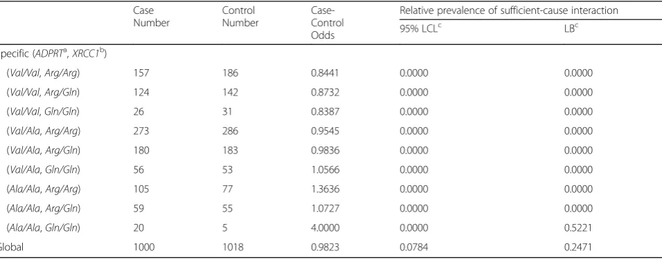
Example 2. A case-control study on lung cancer risk Zhang et al.’s case-control data (directly taken from Table 4 in reference [22]) is analyzed here as the second example. The study examines the gene-gene interactions between two DNA base excision repair genes on lung cancer risk: the ADPRT (adenosine diphosphate ribosyl-transferase) Val762Ala polymorphism and the XRCC1 (X-ray repair cross-complementing group 1) Arg366Gln polymorphism (both having three genotypes). The rare-disease assumption is invoked here (For lung cancer, the assumption is tenable). In addition, we assume gene-environment independence [10] such that unmeasured en-vironmental factors, no matter what they may be, cannot confound the genetic effects of the two studied genes.
Table 2 presents the lower bounds and the 95% lower limits for sufficient-cause interactions between these two genes. The lower bound of the relative prevalence for the (ADPRT=Ala/Ala, XRCC1=Gln/Gln)-specific sufficient-cause interaction is greater than zero (0.5221) but does not achieve statistical significance. The lower bound of the relative prevalence for the global ADPRT -XRCC1 interaction is 0.2471 and is significantly greater than zero (as judged from its 95% lower con-fidence limit which is 0.0784).
Discussion
Public health researchers have long sought a way to quantify sufficient-cause interactions using only the ob-servational data at hand. Due to the non-identifiability problem, a sufficient-cause interaction can be tested but unfortunately not estimated. We are therefore provided with a very limited piece of information (of whether or not a sufficient-cause interaction is statistically signifi-cant), which falls far short of quantification. By setting bounds on sufficient-cause interactions (as demonstrated in the two examples in this paper), we can finally make some actual (if not exact) quantifications of such interactions.
for the cumulative completion risk of the specific class =i,j sufficient-cause interaction (which they called ‘weak’ sufficient-cause interaction). Using the notations of this paper, their bound is
maxi′≠i∈ 1;…;L
1
f g
j′≠j
∈f1;…;L2g
Riskprofile¼i;j−Riskprofile¼i′;j−Riskprofile¼i;j′;0
n o
:
Additional file 4 shows we can achieve a sharper lower bound.
In this paper, the lower bound formulae also provide an avenue for testing of specific sufficient-cause interac-tions; if the bootstrapped 95% lower confidence limits for a particular lower bound is greater than zero, then the corresponding sufficient-cause interaction is present. Alternatively, one can rely on the lower bound for the global sufficient-cause interaction; if its bootstrapped 95% lower confidence limit is greater than zero, then some sufficient-cause interaction (between certain levels of the two factors) must be present. When both expo-sures are binary, such global test reduces to testing
PRISM = 1 against PRISM≠1 in cohort studies [7], and RERI = 0 against RERI≠0 in case-control studies.
The assumption of no confounding is a strong one. To alleviate the problem, the data can be stratified by the confounders (if these are identified and measured in the study) and separate bounds set on sufficient-cause inter-actions using the proposed formulae in this paper for each of the resulting strata. Further work is warranted to develop stratified bounding methods for sufficient-cause interactions when the total number of strata is large and the average stratum size is small (the sparse-data sce-nario) and when some of the stratifying variables also interact with the two exposures of concern (sufficient-cause interactions involving more than two variables).
Conclusions
The study provides bounding formulae for sufficient-cause interactions under the assumption of no redun-dancy. The bounds are sharp and sharper than previous
Table 1Bounds on sufficient-cause interactions in a cohort study on hypertension risk (Example 1)
Case number
Population Risk Cumulative completion risk of sufficient-cause interaction
Relative prevalence of sufficient-cause interaction
95% LCLc LBc UBc 95% UCLc 95% LCLc LBc
Specific (BMIa, ageb)
(low, young) 79 1810 0.0437 0.0000 0.0000 0.0436 0.0530 0.0000 0.0000
(low, old) 100 681 0.1468 0.0000 0.0000 0.1468 0.1733 0.0000 0.0000
(high, young) 153 1385 0.1105 0.0000 0.0000 0.1105 0.1278 0.0000 0.0000
(high, old) 278 1021 0.2723 0.0000 0.0411 0.2723 0.2997 0.0000 0.1509
Global 610 4897 0.1246 0.0338 0.0830 0.4718 0.4993 0.0879 0.1758
a
old: age≥40 years; young: age < 40
b
BMIbody mass index; high: BMI≥25 kg/m2
; low: BMI < 25
c
LCLlower confidence limit for the lower bound,LBlower bound,UBupper bound,UCLupper confidence limit for the upper bound
Table 2Bounds on sufficient-cause interactions in a case-control study on lung cancer risk (Example 2)
Case Number
Control Number
Case-Control Odds
Relative prevalence of sufficient-cause interaction
95% LCLc LBc
Specific (ADPRTa,XRCC1b)
(Val/Val,Arg/Arg) 157 186 0.8441 0.0000 0.0000
(Val/Val,Arg/Gln) 124 142 0.8732 0.0000 0.0000
(Val/Val,Gln/Gln) 26 31 0.8387 0.0000 0.0000
(Val/Ala,Arg/Arg) 273 286 0.9545 0.0000 0.0000
(Val/Ala,Arg/Gln) 180 183 0.9836 0.0000 0.0000
(Val/Ala,Gln/Gln) 56 53 1.0566 0.0000 0.0000
(Ala/Ala,Arg/Arg) 105 77 1.3636 0.0000 0.0000
(Ala/Ala,Arg/Gln) 59 55 1.0727 0.0000 0.0000
(Ala/Ala,Gln/Gln) 20 5 4.0000 0.0000 0.5221
Global 1000 1018 0.9823 0.0784 0.2471
a
ADPRT:adenosine diphosphate ribosyltransferase
b
XRCC1:X-ray repair cross-complementing group 1
c
bounds. Sufficient-cause interactions cannot be estimated but can be quantified using the bounds presented in this study.
Additional files
Additional file 1:Derivations of the bounding formulas. (PDF 272 kb)
Additional file 2:R code. (PDF 151 kb)
Additional file 3:A proof that the bounds are sharp. (PDF 179 kb)
Additional file 4:A proof that the bounds are sharper than previous bounds. (PDF 286 kb)
Abbreviations
ADPRT:Adenosine diphosphate ribosyltransferase; BMI: Body mass index;
LB: Lower bound; PRISM: Peril ratio index of synergy based on multiplicativity; RERI: Relative excess risk due to interaction; RP: Relative prevalence; UB: Upper bound;XRCC1:X-ray repair cross-complementing group 1
Acknowledgements
Not applicable.
Funding
This paper is partly supported by grants from Ministry of Science and Technology, Taiwan (MOST 105-2314-B-002-049-MY3). No additional external funding received for this study. The funders had no role in study design, data collection and analysis, decision to publish, or preparation of the manuscript.
Availability of data and materials
The dataset supporting the conclusions of this article is included within the article and the Additional files.
Author’contributions
This is a single-authorship paper by WCL.
Competing interests
The author declares that he has no competing interests.
Consent for publication
Not applicable.
Ethics approval and consent to participate
Not applicable.
Publisher’s Note
Springer Nature remains neutral with regard to jurisdictional claims in published maps and institutional affiliations.
Received: 29 November 2016 Accepted: 12 April 2017
References
1. VanderWeele TJ, Robins JM. The identification of synergism in the sufficient-component cause framework. Epidemiology. 2007;18:329–39.
2. VanderWeele TJ, Robins JM. Empirical and counterfactual conditions for sufficient cause interactions. Biometrika. 2008;95:49–61.
3. VanderWeele TJ. Sufficient cause interactions and statistical interactions. Epidemiology. 2009;20:6–13.
4. VanderWeele TJ. Sufficient cause interactions for categorical and ordinal exposures with three levels. Biometrika. 2010;97(3):647–59.
5. VanderWeele TJ, Knol MJ. Remarks on antagonism. Am J Epidemiol. 2011; 173:1140–7.
6. Lee WC. Testing synergisms in a no-redundancy sufficient-cause rate model. Epidemiology. 2013;24(1):174–5.
7. Lee WC. Assessing causal mechanistic interactions: a peril ratio index of synergy based on multiplicativity. PLoS ONE. 2013;8(6):e67424. 8. Lee WC. Estimation of a common effect parameter from follow-up data
when there is no mechanistic interaction. PLoS ONE. 2014;9:e86374.
9. Lin JH, Lee WC. Testing for mechanistic interactions in long-term follow-up studies. PLoS ONE. 2015;10:e0121638.
10. Lee WC. Testing for sufficient-cause gene-environment interactions under independence and Hardy-Weinberg equilibrium assumptions. Am J Epidemiol. 2015;182(1):9–16.
11. Lee WC. Excess relative risk as an effect measure in case-control studies of rare diseases. PLoS ONE. 2015;10(4):e0121141.
12. Rothman KJ. Causes. Am J Epidemiol. 1976;104:587–92.
13. Rothman KJ, Greenland S, Lash TL, editors. Modern Epidemiology. 3rd ed. Philadelphia: Lippincott; 2008.
14. Greenland S, Brumback B. An overview of relations among causal modelling methods. Int J Epidemiol. 2002;31(5):1030–7.
15. Liao SF, Lee WC. Weighing the causal pies in case-control studies. Ann Epidemiol. 2010;20(7):568–73.
16. Suzuki E, Yamamoto E, Tsuda T. On the link between sufficient-cause model and potential-outcome model. Epidemiology. 2011;22(1):131–2.
17. Suzuki E, Yamamoto E, Tsuda T. On the relations between excess fraction, attributable fraction, and etiologic fraction. Am J Epidemiol. 2012;175(6):567–75. 18. Lee WC. Completion potentials of sufficient component causes.
Epidemiology. 2012;23(3):446–53.
19. Gatto NM, Campbell UB. Redundant causation from a sufficient cause perspective. Epidemiol Perspect Innov. 2010;7:5.
20. Sjölander A, Lee W, Källberg H, Pawitan Y. Bounds on sufficient-cause interaction. Eur J Epidemiol. 2014;29:813–20.
21. Zou GY. On the estimation of additive interaction by use of the four-by-two table and beyond. Am J Epidemiol. 2008;168:212–24.
22. Zhang X, Miao X, Liang G, Hao B, Wang Y, Tan W, Li Y, Guo Y, He F, Wei Q, Lin D. Polymorphisms in DNA base excision repair genes ADPRT and XRCC1 and risk of lung cancer. Cancer Res. 2005;65:722–6.
• We accept pre-submission inquiries
• Our selector tool helps you to find the most relevant journal • We provide round the clock customer support
• Convenient online submission • Thorough peer review
• Inclusion in PubMed and all major indexing services • Maximum visibility for your research
Submit your manuscript at www.biomedcentral.com/submit
![Table 4 in reference [22]) is analyzed here as the second](https://thumb-us.123doks.com/thumbv2/123dok_us/9309442.1918239/4.595.69.292.87.203/table-reference-analyzed-second.webp)