© 2017, IRJET | Impact Factor value: 5.181 | ISO 9001:2008 Certified Journal | Page 3210
STUDIES ON MACHINING PARAMETERS OF HOT MACHINING PROCESS
USING AISI4140 MATERIAL
Jagjit Singh
M. Tech. Mechanical Engineering, LR Institute of Engineering & Technology Solan, H.P, India
---***---Abstract -
The experiment is conducted on conventional lathe. The temperature is controlled by a infra -rate thermometer and flame heating system. The statistical analysis is done by Taguchi method. Taguchi designs provide a powerful and efficient method for designing products that operate consistently and optimally over a variety of conditions. The primary goal is to find factor settings that minimize response variation, while adjusting the process on target. A process designed with this goal will produce more consistent output. A product designed with this goal will deliver more consistent performance regardless of the environment in which it is used. Taguchi method advocates the use of orthogonal array designs to assign the factors chosen for the experiment. The L9 orthogonal array of a Taguchi experiment is selected for fourparameters (speed, feed rate, depth of cut and temperature) with three levels (low, medium, andhigh) in optimizing the hot machining turning parameters on lathe.Key Words:
Surface roughness, MRR (Material removalrate), Orthogonal array, Analysis ofvariance (ANOVA), Grey-Taguchi Technique
.
1 INTRODUCTION
The basic of hot machining operation is to first soften the work piece is by preheating and thereby shear strength gets reduced in the vicinity of the shear zone. The use of hot machining has become very useful in the machining of high strength temperature-resistant (HSTR) alloys. Hot machining has two functions to perform, one, to machine some HSTR alloys which are un Machninable in the conventional machining method. Second, to improve tool life this eventually improves the production rate. There are various techniques of hot machining which are subjected to requirements. The penetration of heat should be such that the shear zone is appreciably affected. Input rate of heat must be commendably high, so as to temperature sufficiently and quickly. Thermal damage done to work piece through distortion should be minimum. The installation and operation cost should be minimum. The operators in the operation should take safety measures into account. Temperature control should be quickly obtained. The obtained results indicatethat the feed rate was found to be the dominant factor among controllable factors on the surface roughness, followed by depth of cut and tool’s nose radius. However ,the cutting speed showed an insignificant effect. Furthermore, the interaction of feed rate/depth of cut
was found to be significant on the surface finish due to surface hardening of steel.
1.1
DIFFERENT METHODS OF HEATING
Different heating methods use for heating work piece in hot machining are
1.1.1 Furnace heating
Work piece is machined immediately after being heated in the furnace to required temperature.
1.1.2 Resistance heating
The entire work piece is heated by passing current either through the work piece itself or through resistance heaters embedded in the fixtures.
1.2.3 Flame heating
In this method, work piece material immediately ahead of the cutting tool is heated by welding torch moving with the tool. Multi-flame heads can be used for large heat inputs.
1.2.4 Arc heating:
In this method, the work piece material immediately ahead of the cutting tool is heated by an electric arc drawn between the work piece and the electrode moving with the tool. To prevent wandering a magnetic field can be imposed to direct the arc.
1.2.5 Plasma arc heating:
In this method, the work piece is heated using plasma arc just above the tool tip. In this method very high heat is produced. Heating can be limited to a very small surface area.
1.2
CUTTING TOOLS
The most common tool materials that are used include the following:
© 2017, IRJET | Impact Factor value: 5.181 | ISO 9001:2008 Certified Journal | Page 3211 3. Carbon steel
4. Cobalt high speed steel
Tool Holder: - WIDAX- PCLNR 2525 M 12 D 5F with 20 mm Shank.
Insert: - Kennametal insert with Grade: KC5525 ISO catalogue number:- CNMG120408RP ANSI catalogue number: - CNMG432RP
1.3
CUTTING PARAMETERS
In turning, the speed and motion of the cutting tool is specified through several parameters. These parameters are selected for each operation based upon the work piece material, tool material, tool size, and more.
Speed
Always refers to the spindle and the work piece. When it is stated in revolutions per minute (rpm) it tells their rotating speed. But the important feature for a particular turning operation is the surface speed, the speed at which the work piece material is moving past the cutting tool. It is simply the product of the rotating speed times the circumference of the work piece before the cut is started. It is expressed in meter per minute (m/min), and it refers only to the work piece. Every different diameter on a work piece will have a different cutting speed, even though the rotating speed remains the same.
[1.1]
Where, v is the cutting speed in turning, D is the initial diameter of the work piece in mm and N is the spindle speed in RPM.
Feed
Always refers to the cutting tool, and it is the rate at which the tool advances along its cutting path. On most power-fed lathes, the feed rate is directly related to the spindle speed and is expressed in mm (of tool advance) per revolution (of the spindle), or mm/rev.
Fm= f. N mm/Min [1.2]
Where, Fm is the feed in mm per minute, f is the feed in mm/rev and N is the spindle speed in RPM.
Depth of cut
Is practically self explanatory. It is the thickness of the layer being removed (in a single pass) from the work piece or the distance from the uncut surface of the work to the cut surface, expressed in mm. It is important to note, though, that the diameter of the work piece is reduced by two times the depth of cut because this layer is being removed from both sides of the work.
[1.3] Where, D and d represent initial and final diameter (in mm) of the job respectively.
1.4
ABOUT ANALYSIS SOFTWARE MINITAB 15
Minitab software is a statistics package used for analysis of experimental data. It was developed at the Pennsylvania State University by researchers Barbara F. Ryan, Thomas A. Ryan, Jr., and Brian L. Joiner in 1972. The goal of robust experimentation is to find an optimal combination of control factor settings that achieve robustness against (insensitivity to) noise factors. MINITAB 15 calculates response tables and generates main effects and interaction plots for Signal-to-noise ratios (S/N ratios) vs. the control factors. It provides standard orthogonal array for Taguchi methodology for experiment design. It also performs regression analysis to establish relation between two or more variables. It also helps in generating various types of tables and graphs.
2. EXPERIMENTAL SETUP
2.1 Work piece material:
For performing hot machining, the selected material should be hard enough that at elevated temperature it should maintain the strength. Considering this, AISI 4140 as a work piece material is selected. The material is in the form of round bar and having mm diameter and mm length The material is heat treated by tempering at and oil quenched and having hardness of 50 HRc (Rockwell hardness). The Chemical, Physical and Mechanical properties of material are shown below.
Table- 1: Chemical composition of AISI 4140 steel materials
Material C Mn Si Cr Mo P S
AISI
4140 .35
to
.45 .45
to
.70 .10
to
.80 1.00
to
1.45 0.25
to 0.40
0.035 0.040
Table- 2: Physical properties
Material Density
gm/cm
Melting Point
(ºC )
Thermal Conductivity
at 100 ºC
( W/m k )
Coefficient of
Thermal expansion
( µm )/m ºC
AISI
© 2017, IRJET | Impact Factor value: 5.181 | ISO 9001:2008 Certified Journal | Page 3212 Table- 3: Mechanical properties
Material Tensile strength
( MPa)
Yield Strength
( MPa)
% Elongation
4140 1050 685 14
Table- 4: Insert Dimension
D L10 S Rɛ D1
Mm 12.75 13.00 4.75 0.85 5.16
Inch ½ 0.508 3/16 1/32 0.202
2.1.2 Turning Machine:
The machine used for hot machining is Conventional lathe made by HMT Machinery stores.
Coil Volts = 110 Full load Amps = 48
Cycle = 50 H.P. = 3 Phase = 3 Speed Range =50-1225 rpm
Feed Range = 0.05 – 0.715 mm/revolution
Fig- 2.1:
Experiment Setup
2.2 TAGUCHI METHOD FOR SINGLE OBJECTIVE
OPTIMIZATION FOR EXPERIMENTAL RESULT
Taguchi’s methods of experimental design provide a simple, efficient, and systematic approach for the optimization of experimental designs for performance quality and cost. The main purpose of Taguchi method is reducing the variation in a process through robust design of experiments. It was developed by Dr. Genichi Taguchi of Japan. He developed a method for designing experiments to investigate how different parameters affect the mean and variance of a
process performance characteristic that defines how well the process is functioning. The experimental design proposed by Taguchi involves using orthogonal arrays to organize the parameters affecting the process and the levels at which they should be varied; it allows for the collection of the necessary data to determine which factors most affect product quality with a minimum amount of experimentation, thus saving time and resources. Analysis of variance on the collected data from the Taguchi design of experiments can be used to select new parameter values to optimize the performance characteristic.
2.2.1 Process steps of Taguchi method
1. Define the process objective 2. Identify test conditions
3. Identify the control factors and their alternative levels 4. Create orthogonal arrays for the parameter design 5. Conduct the experiments indicated in the completed array to collect data on the effect on the performance measure. 6. Complete data analysis to determine the effect of the different parameters on the performance measure. 7. Predict the performance at these levels
8. Confirmation experiments.
2.1.2 Signal -to- Noise (S/N) ratio
The objective of problem statement is to obtain maximum value or minimum value of desired response. Taguchi method chooses to calculate the signal-to-noise ratio for finding effective parameter for desire response value. To calculate the S/N ratio, experiments are conducted in a systematic manner Taguchi’s idea is to recognize controllable and noise factors and to treat them separately as a design parameter matrix and a noise factor matrix, respectively. Experiments are organized according to orthogonal arrays (OAs). Noise factors are changed in a balanced fashion during experiments.
The characteristics of S/N ratio can be divided into three categories smaller is better, Higher is better and nominal is best when the characteristic is continuous.
These characteristics are selected as per objective of problem. They are calculated by following equation.
(a) Nominal is the best characteristic
(2.1)
(b) Smaller is better
(2.2)
(c) Larger the better characteristic
© 2017, IRJET | Impact Factor value: 5.181 | ISO 9001:2008 Certified Journal | Page 3213
(2.4)
=
(2.5)
I = Experiment number u = Trial number
Ni = Number of trials for experiment i.
The effect of many different parameters on the performance characteristic in a condensed set of experiments can be examined by using the orthogonal array. Once the parameters affecting a process that can be controlled have been determined, the levels at which these parameters should be varied must be determined. Determining what levels of a variable to test requires an in-depth understanding of the process, including the minimum, maximum, and current value of the parameter. If the difference between the minimum and maximum value of a parameter is large, the Values being tested can be further apart or more values can be tested. If the range of a parameter is small, then fewer values can be tested or the values tested can be closer together.
A matrix has a number of columns equal to the number of factors (parameters) to be considered, each column representing a specific factor. Within each column we specify the levels (parameter setting) at which the factors are kept for experiments. The number of rows in a matrix represents the number of experiments that are to be performed. As the name suggests, the columns or orthogonal array are mutually orthogonal. Here, orthogonal is interpreted in the combinatory sense that is for any pair of columns, all combinations of factor levels appear equal number of times. An orthogonal array design gives more reliable estimates of factor effects with fewer experiments that are needed in traditional methods.
Taguchi has tabulated 18 basis orthogonal arrays. An arrays name indicates the number of rows and columns it has and also the number of levels in each columns. For example L12
(211) has 12 rows and 11 columns each at 2 levels. The array
can be directly used in many cases or modified to suit a specific problem. The number of rows of an orthogonal array represents the number of experiments. For an array to be a viable choice, the number of rows must be at least equal to the degrees of freedom required for the case study. The number of columns of an array represents the maximum number of factors that can be studied using that array. Usually, it is expensive to conduct experiments of the case study. The selection orthogonal arrays for number of process parameter with respect to levels of variation of parameter are listed in the table given below table no. 3.1 Analysis of variance techniques provides a mathematical basis for organizing and interpreting the experimental results. For each performance requirement, signal-to-noise (S/N) ratio is used. The cutting parameter range is suggested by the
cutting tool manufacturers. Based on that, in this experiment each parameter is varied by three different levels.
2.3 SELECTION OF PROCESS VARIABLE
In today’s market, productivity, surface finish and longer tool life are most important factors for manufacturing industry. From past literature survey it is found that several factors influence the surface roughness, material removal rate and tool wear in a turning operation. The theoretical surface roughness is generally dependent on many parameters such as the tool material, work material, tool geometry (tool nose radius, flank, tool runoff) machine-tool rigidity and various cutting conditions including feed rate, depth of cut and cutting speed. However, factors such as tool wear, chip loads and chip formations, or material properties of both tool and work piece are uncontrollable during actual machining. The presence of chatter or vibration of the machine tool, defects in the surface of work material, wear in the tool or irregularities of chip formation contribute to the surface damage in practice during actual machining operations. In study of effect of parameter in investigation it is not possible consider all parameter at same time. So in this work cutting speed, Feed, depth of cut and temperature is taken as turning process variable parameter. The cutting parameter range is suggested by the cutting tool manufacturers. Based on that, in this experiment each parameter is varied by three different levels.
Table-5 : Control Factors and Their Range of Setting for the Experiment
Control
Variable
Cutting speed
(m/min)
Feed
(mm/rev)
Depth of cut
(mm)
Temperature
Level-1 30 .10 .04 55
Level-2 80 .15 .06 110
Level-3 125 .20 .08 220
2.3.1 Selection of arrays
Table- 6: Experiment design by use of L9 Orthogonal array
Sr.No Parameter
1 Parameter 2 Parameter 3 Parameter 4
1 1 1 1 1
2 1 2 2 2
© 2017, IRJET | Impact Factor value: 5.181 | ISO 9001:2008 Certified Journal | Page 3214
4 2 1 2 3
5 2 2 3 1
6 2 3 1 2
7 3 1 3 2
8 3 2 1 3
9 3 3 2 1
The final experiment are designed by proving selected parameters values as per Table 4.6, suggested by tool maker company’s technical specification catalog and hand book of production technology in Minitab- 15 statistical software is shown in Table 7.
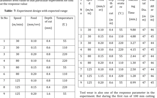
[image:5.595.30.293.98.233.2]The experiment suggested by this table is specifying the parameter level value of that particular experiment for find out the response value
Table- 7:
Experiment design with expected range
Sr.No Speed
(m/min)
Feed
(mm/rev)
Depth of cut
(mm)
Temperature
1 30 0.10 0.4 55
2 30 0.15 0.6 110
3 30 0.20 0.8 220
4 80 0.10 0.6 220
5 80 0.15 0.8 55
6 80 0.20 0.4 110
7 125 0.10 0.8 110
8 125 0.15 0.4 220
9 125 0.20 1.6 55
2.4 Experimentation
a. Prepare the set up of hot machining i.e. mounting of nozzle on tool carriage opposite of cutting tool to provide moving flow of heat.
b. Mount the work piece on lathe chuck. And measure the initial work piece diameter.
c. Mount the tool holder on tool post.
d. Set the required combination of speed and feed.
e. Set the regulator pressure, start the machine and then start the flame.
f. Adjust the flow of oxygen and acetylene in such a way that work piece is heated well.
g. Give manual heating to the whole work piece without machining, to pre-heat the work piece by moving carriage hand wheel in forward and backward direction.
h. Measure the temperature using optical pyrometer. i. When the temperature reaches slightly above the required temperature, set the parameter and start machining. j. During machining maintain the temperature of work piece by adjusting flow of heat from nozzle regulator.
k. Measure the machining time and diameter of work piece after machining.
[image:5.595.41.567.332.662.2]l. Repeat the procedure for all parameter combination.
Table -8:
Experiment Table 1
S r.
N o
Spee d
(m/m in)
Feed
(mm/r ev)
Dep th of
cut
(m m)
Temp eratu re
Machin
ing
Time
(min.) Init
ial
Dia.
(m m)
Dia.
Aft er
(m m)
1 30 0.10 0.4 55 9.80 47 46
2 30 0.15 0.6 110 4.88 47 45
3 30 0.20 0.8 220 3.27 47 44
4 80 0.10 0.6 220 4.15 47 45
5 80 0.15 0.8 55 2.44 47 44
6 80 0.20 0.4 110 1.30 47 46
7 125 0.10 0.8 110 2.50 47 44
8 125 1.15 0.4 220 1.28 47 46
9 125 0.20 0.6 55 0.99 47 45
Tool wear is also one of the response parameter in the experiment. But during the first run of 100 mm cutting length, there is no effect (non measurable) found regarding tool wear. So for measurable tool wear second run of same parameter is repeated and then effect on surface roughness, material removal rate and tool wear is observed.
3 RESULTS
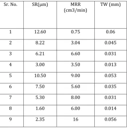
© 2017, IRJET | Impact Factor value: 5.181 | ISO 9001:2008 Certified Journal | Page 3215 material removal rate (in mm3/min) and tool wear (in
[image:6.595.36.293.156.416.2]mm) measured are shown in table 8.
Table- 9: Result table for SR, MRR and TW
Sr. No. SR μm MRR
(cm3/min) TW (mm)
1 12.60 0.75 0.06
2 8.22 3.04 0.045
3 6.21 6.60 0.031
4 3.00 3.50 0.013
5 10.50 9.00 0.053
6 7.50 5.60 0.035
7 5.30 8.00 0.031
8 1.60 6.00 0.014
9 2.35 16 0.056
The analyzed value of S/N ratio for surface roughness by use Minitab15 statistical software is shown in Table 10.
Table- 10:
S/N ratio calculation of SR
Ex.
No. S/N Ratio of SR
1 -21.0134
2 -18.4029
3 -14.9166
4 -8.23686
5 -21.5786
6 -17.5703
7 -15.2201
8 -3.51172
9 -19.2117
3.1 Main effects plot of surface roughness
[image:6.595.310.570.233.372.2]The main effects plot for S/N ratio of surface roughness verses cutting speed, feed rate, depth of cut and temperature, which is generate form the value of S/N ratio of surface roughness as per Table 9. in Minitabe-15 statistical software is useful to find out optimum parameter value for response variable. The graph generate by use of Minitab-15 statistical software for surface roughness is shown in graph 3.1.
Fig.-3.1: Mean effect plot of surface roughness vs. Cutting speed, Feed, DOC andTemperature
From the Figure 3.1 it is conclude that the optimum combination of each process parameter for lower surface roughness is meeting at high cutting speed (A3), medium feed rate (B2), low depth of cut (C1), and high temperature (D3). The S/N of the surface roughness for each level of the each machining parameters can be computed in Minitab 15 and it is summarized for finding out rank of each effective parameter for response.
The analyzed value of mean of surface roughness by use of Minitab 15 statistical software is shown in Table 10.
Table -11: Response table of S/N ratio for surface roughness
Level Speed Feed DOC Temp.
1 -18.781 -15.183 -14.269 -20.607
2 -15.765 -14.131 -15.881 -16.654
3 -12.385 -16.991 -16.909 - 9.462
Delta -5.993 -3.361 2.530 12.045
Rank 2 3 4 1
© 2017, IRJET | Impact Factor value: 5.181 | ISO 9001:2008 Certified Journal | Page 3216 12.045 for surface roughness. From delta value of each
parameter it is conclude that for surface roughness the most effective parameter is Temperature followed by cutting speed, feed rate and depth of cut.
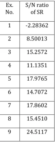
[image:7.595.116.209.208.445.2]3.2 Main effects plot of material removal rate
:Table- 12:
S/N ratio calculation of MRR
Ex.
No. S/N ratio of SR
1 -2.28362
2 8.50013
3 15.2572
4 11.1351
5 17.9765
6 14.7072
7 17.8602
8 15.4510
9 24.5117
The main effects plot of material removal rate verses cutting speed, feed rate, depth of cut and temperature, The S/N of the material removal rate for each level of the each machining parameters can be computed in Minitab 15. which is generate form the value of S/N ratio of material removal rate in Minitabe-15 statistical software is useful to find out optimum parameter value for response variable. The graph generate by use of Minitab-15 statistical software for material removal rate is shown in figure 3.2.
Fig-3.2: Mean effect plot of material removal rate vs. Cutting speed, Feed, DOC and Temperature
From the figure 3.2 it is conclude that the optimum combination of each process parameter for higher material removal rate is meeting at high cutting speed (A3), high feed rate (B3), high depth of cut (C3), and medium temperature (D2).
The S/N of the material removal rate for each level of the each machining parameters can be computed in Minitab 15.
4. MAIN EFFECTS PLOT OF GREY RELATIONAL
GRADE
[image:7.595.308.570.350.508.2]The following graph shows the main effects plot for GRG. Basically, the larger the grey relational grade, the better is the multiple performance characteristic. For the combined responses maximization or minimization, graph gives optimum value of each control factor hart interprets that Level of utting speed m min , eed rate mm rev , epth of cut mm and Temperature gives optimum result
Fig -3.3: Mean effect plot of grey relational grade vs. Cutting speed, Feed rate, Depth of cut and Temperature
The effect of each hot turning process parameter on the grey relational grade at different levels can be independent because the experimental design is orthogonal. The mean of the grey relational grade for each level of the hot turning process parameters is summarized and shown in following Table. In addition, the total mean of the grey relational grade for the 8 experiments is calculated and listed in following Table 8.
Table -13: Mean effects factors on grey relational grade
Level Speed Feed DOC Temp.
1 -7.709 -5.706 -7.062 -8.144
2 -5.610 -5.737 -6.075 -7.567
© 2017, IRJET | Impact Factor value: 5.181 | ISO 9001:2008 Certified Journal | Page 3217
5. TEST
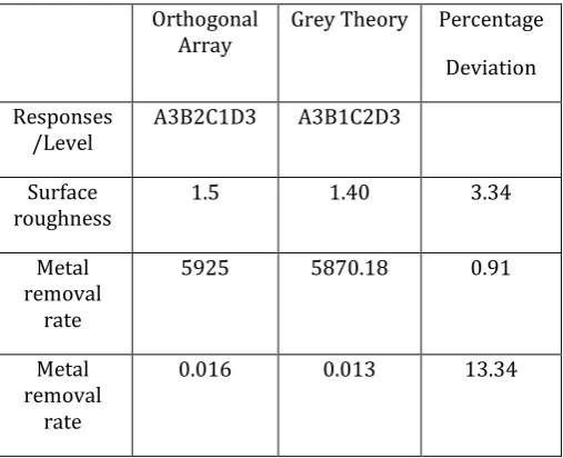
The final step in the experiment is to do confirmation test. The purpose of the confirmation runs is to validate the conclusion drawn during the analysis phases. In addition, the confirmation tests need to be carried out in order to ensure that the theoretical predicted parameter combination for optimum results using the software was acceptable or not. The parameters used in the confirmation test are suggested by grey relational analysis. The confirmation test with optimal process parameters is performed at levels A3, B1, C2, D3 of process parameter takes 2.51 minute time for 100 mm length of cut and gives 1.4 μm value, mm min material removal rate and 0.013mm tool wear is obtained.
Table -14: Optimization results of orthogonal array Vs Grey theory design
Orthogonal
Array Grey Theory Percentage Deviation
Responses
/Level A3B2C1D3 A3B1C2D3
Surface
roughness 1.5 1.40 3.34
Metal removal
rate
5925 5870.18 0.91
Metal removal
rate
0.016 0.013 13.34
6. CONCLUSION
6.1 Surface Roughness
Best parameter combinations for optimum surface roughness are: Speed (A) at level 3 (125 m/min), feed (B) at level 2 (0. mm rev , epth of cut at level mm and temperature at level
6.2 Material Removal Rate
1. Cutting speed is the most significant parameter for higher material removal rate value followed by feed, depth of cut and temperature.
est parameter combinations for optimum material removal rate are Speed at level m min , feed at level mm rev , epth of cut at level mm and temperature at level
6.3 Tool Wear
1. Temperature is the most significant parameter for lower tool wear value followed by feed, speed and depth of cut. 2. Best parameter combinations for optimum tool wear are: Speed (A) at level 2 (80 m/min), feed (B) at level 1 (0.10 mm/rev), Depth of cut (C) at level 1 (0.4 mm) and temperature at level
Based on Grey Relational Analysis, for optimum surface roughness, material removal rate and tool wear, the temperature is most significant parameter followed by speed, depth of cut and feed.
The optimal process parameters, for surface roughness, material removal rate, and tool wear, based on grey relational analysis are high cutting speed m min , low feed mm rev , medium depth of cut mm and pre-heating temperature of
By using Grey Taguchi analysis, the surface roughness increased by 3.34% and material removal rate and tool wear improves by 0.91 % and 13.34% respectively.
7. FUTURE SCOPE
The present work concentrated on optimization of turning process parameter in Hot Machining. The variables to be altered are cutting speed, feed, depth of cut and temperature of work piece. The parameters to optimize are taken as surface roughness, material removal rate and tool wear. The experiment is conducted on conventional lathe. Flame heating technique is used to preheat the work piece. 1.The same experiment can performed by changing parameter i.e. by taking parameters like tool geometry, tool run off, work piece material etc. or by taking different level of process parameter. Here also higher temperature level can be selected, to observe the clear effect of temperature on machining.
2. The tool wear criteria can be extended and tool life can also be found out. Also equation of tool life can be developed in terms of process parameters.
REFERENCES
[1] N. Tosun and Ozler L , “Optimization for hot turning operations with multiple performances characteristic”,
International Journal of Advanced ManufacturingTechnology, (2004), Vol. 23, pp. 777-782.
[ ] Nikunj R Modh, G Mistry and K Rathod, “ n experimental investigation to optimize the process parameter of ISI steel in hot machining”,
International journal of engineering research and application,
Vol, 1, Issue 3, pp.- 483-489.
[image:8.595.39.293.311.517.2]© 2017, IRJET | Impact Factor value: 5.181 | ISO 9001:2008 Certified Journal | Page 3218 [4] R. D. Rajopadhye, M. T. Telsang and N. S. Dhole,
“Experimental setup for hot machining process to increase tool life with torch flame”, IOSR journal ofmechanical and civil engineering, pp.-58-62.
[ ] G S Kainth, ey K ,” n experimental investigation into cutting forces and chip tool interface temperature for oblique hot machining of EN 24 steel”, BulletinCercle Etudes des Métaux, (1980), pp-22.1-22.7.
[ ] Ketul M Trivedi and Jayesh V esai, “ n experimental investigation to optimize the process parameters of AISI steel in hot machinig”, International journal for scientific research & development, March (2014), Vol. 2, Issue 03, pp.-1542-1545.
[ ] K Patel, S Patel and K Patel, “Performance evaluation and parametric optimization of hot machining process on EN- material”, International journal for technological research in engineering, June (2014), Volume 1, Issue 10, pp.-1265-1268.
[ ] K P Maity and, P K Swain, “ n experimental investigation of hot-machining to predict tool life”, Journal of materials processing technology 198, (2008), pp.344–349.
[9] Jacques Goupy and Lee Creighton, Introduction to Design of Experiments with JMP® Examples, Third Edition, SAS publish, USA.
[10] Douglas C Montgomery, Design and Analysis of Experiments, 7th edition.
[11] Jiju Antony, Design of Experiments for Engineers and Scientists, Elsevier Science & Technology Books, October 2003.
[ ] G Taguchi, “introduction to Quality Engineering, sian Productivity organization”, Tokyo, 99