Open Access
Technical advance
Fitting multilevel models in complex survey data with design
weights: Recommendations
Adam C Carle
Address: Department of Psychology, University of North Florida, 1 UNF Drive, Jacksonville, FL, 32224, USA
Email: Adam C Carle - [email protected]
Abstract
Background: Multilevel models (MLM) offer complex survey data analysts a unique approach to understanding individual and contextual determinants of public health. However, little summarized guidance exists with regard to fitting MLM in complex survey data with design weights. Simulation work suggests that analysts should scale design weights using two methods and fit the MLM using unweighted and scaled-weighted data. This article examines the performance of scaled-weighted and unweighted analyses across a variety of MLM and software programs.
Methods: Using data from the 2005–2006 National Survey of Children with Special Health Care Needs (NS-CSHCN: n = 40,723) that collected data from children clustered within states, I examine the performance of scaling methods across outcome type (categorical vs. continuous), model type (level-1, level-2, or combined), and software (Mplus, MLwiN, and GLLAMM).
Results: Scaled weighted estimates and standard errors differed slightly from unweighted analyses, agreeing more with each other than with unweighted analyses. However, observed differences were minimal and did not lead to different inferential conclusions. Likewise, results demonstrated minimal differences across software programs, increasing confidence in results and inferential conclusions independent of software choice.
Conclusion: If including design weights in MLM, analysts should scale the weights and use software that properly includes the scaled weights in the estimation.
Background
IntroductionMultilevel models (MLM) offer analysts of large scale, complex survey data a relatively new approach to under-standing individual and contextual influences on public health. Complex sampling designs organize populations into clusters (e.g., states or counties) and then collect data within the clusters. For example, a survey may first identify clusters (e.g., all counties within an area), sample the
clus-ters (i.e., select some but not all of the counties), and then select units within the clusters (e.g., people within a county). These sampling plans result in non-independent data. People within the clusters tend to be more similar to each other than they are to people in other clusters. This can result in biased standard errors and parameters when analyzed using analytical techniques that do not take the clustered nature of the data into account. This, in turn, can lead to increased Type I errors, causing analysts to
incor-Published: 14 July 2009
BMC Medical Research Methodology 2009, 9:49 doi:10.1186/1471-2288-9-49
Received: 8 October 2008 Accepted: 14 July 2009 This article is available from: http://www.biomedcentral.com/1471-2288/9/49
© 2009 Carle; licensee BioMed Central Ltd.
rectly reject null hypotheses. [1-10] Analysts have tradi-tionally used techniques that treat the clustered nature of complex survey data as a nuisance by adjusting the stand-ard errors for the sampling design. This method delivers correct standard errors and properly accounts for non-independence. However, it fails to allow analysts to exam-ine the amount of between-cluster variance unaccounted for by predictors included in the model. [11-14] As public health research becomes increasingly interested in contex-tual influences on health (e.g., state or neighborhood level influences on health), analysts need to adopt meth-ods that allow investigations of variance within and between clusters. [14,15]
MLM offer a unique solution to this problem. They take into account the clustered nature of the data and they allow analysts to investigate sources of variations within and across clusters. Thus, they allow analysts to describe which variables predict individual differences, they allow analysts to describe which variables predict cluster level differences (e.g., state level differences), and they allow analysts to explore variation across and within clusters. Moreover, because MLM explicitly model the clustered nature of the data, MLM can correctly estimate standard errors and lead to more accurate inferential decisions. [16,17] Traditional programs for analyzing complex sur-vey data (e.g., SUDAAN)[18] use program commands to correct the standard errors for the sampling design, but treat the sampling design as a nuisance. In MLM, one expresses the sampling design as part of the equations in the model (Appendix C presents a series of MLM equa-tions), rather than expressing the design outside the model. [17] In this way, analysts can investigate variance within and across clusters.
However, despite the unique contribution MLM can make to understanding public health, [11] they have not been widely adopted by analysts using complex survey data. Limited adoption occurs for several reasons. First, com-plex survey designs often involve unequal selection prob-abilities of clusters and/or people within clusters. The surveys include design (sampling) weights to account for unequal selection probabilities. MLM analyses that incor-porate sampling weights use a pseudomaximum likeli-hood estimation approach. [19] Because the level-1 and level-2 weights appear in separate places within the pseu-domaximum likelihood estimator function, it is not suffi-cient to know the product of the level-1 and level-2 weights. [20] Thus, one must take special care to include design weights. Yet, until recently, few guidelines existed for incorporating design weights into multilevel models. Second, software programs have only begun to correctly include design weights in MLM estimation. Third, little work with empirical (as opposed to simulated) data has compared and contrasted different methods for handling
design weights. And, fourth, few explorations have com-pared the performance of the methods across the major software programs for MLM that allow incorporation of design weights.
In this paper, I take a non-mathematical approach and seek to address these issues. First, I briefly summarize the results of simulation studies and suggest a current best practice recommendation with regard to handling design weights in MLM. Second, I compare and contrast the results of different methods for incorporating sampling weights across a series of MLM using continuous and cat-egorical outcomes and level-1 (individual) and level-2 (cluster) predictors in empirical data across three of the main MLM software programs: Mplus,[21] MLwiN,[22] and GLLAMM. [23] Third, in Appendix A, I provide exam-ple weight-scaling code so that readers can replicate and extend these findings in their own data. Finally, I con-clude with some comments on the strengths and weak-nesses of each software program and summarize some of the remaining methodological issues.
Incorporating Design Weights in Multilevel Models
Summary of Simulation Work
Complex sampling designs regularly incorporate unequal selection probabilities. Failing to account for this aspect of the design in the standard MLM can lead to biased param-eter estimates. [10,20] Thus, while the standard MLM can properly estimate parameters and standard errors in clus-tered data that resulted from equal probability sam-pling,[16,17] the standard MLM may lead to biased estimates when employed in samples that include une-qual probability of selection. To rectify this problem, ana-lysts have recommended incorporating design weights in the likelihood function. [1-10,20,24] The design weights account for unequal selection probabilities. As numerous authors have discussed, though, when estimating MLMs, to properly include design weights in the likelihood func-tion requires scaling the weights. One cannot simply use the "raw" weights. [1-10,20,24] To address this, numer-ous scaling methods have been proposed[1-3,9,10] and analysts have undertaken simulation work to examine the behavior of the scaling methods in simulated data in attempt to identify a scaling method that provides the least biased estimates in most situations[1-3,10,20] (In an effort to focus on analytical application, I do not review the mathematics associated with this work. For further discussion on the mathematical derivations associated with this work, readers should consult Asparouhov [1-3] or Rabe-Hesketh and Skrondal[10]).
appear to provide the least biased estimates in general. [1] Method A,[1] scales the weights so that the new weights sum to the cluster sample size. Method B,[1] scales the weights so that the new weights sum to the effective clus-ter size. These methods have received various labels in the literature. For consistency, I use Asparouhov's [1] labels. Third, no gold standard scaling method has emerged. This transpires because the simulation studies all show that that various features of the design and data can affect a scaling method's adequacy. [1-3,10,20] For example, as cluster sizes increase, the estimates generally become less biased. [1,9,10] This suggests that with sufficiently sized clusters, an analyst may worry less about scaling the weights. Yet, because the number of clusters, the size of the clusters, the type of outcome (categorical vs. continu-ous), the size of the correlation between the outcome and design weight, and the design weights' informativeness can all independently and jointly affect a scaling method's results, a priori scaling method decisions can be difficult. [1]
Fourth, the simulations point to a need for some type of scaling if using weights, especially with small cluster sizes. If one cannot scale the weights and include them properly in the estimation, analyzing the data without weights pro-vides the next best option. Including the weights but fail-ing to scale them (i.e., includfail-ing them as "raw" weights results in biased parameters and standard errors, espe-cially with small cluster sizes. [10] Fifth, as these research-ers note,[10] few publicly available data include weights for each level of analysis. Rather, publicly available data usually include a single overall level-1 weighting variable that incorporates level-2 design issues. This confounding of level-1 (individual) and level-2 (cluster) design issues in a single weight can result in biased estimates. [10] Thus, along with choosing the appropriate scaling method, one must also decide whether to use the "level -1" weights to estimate higher level weights or whether to leave the higher levels unweighted. However, the choice of the scal-ing of the level-2 weights will not influence parameter estimates or the standard errors associated with these esti-mates if level 2 corresponds to the highest level of the model and the same scale factor applies to all units. [3,10] Finally, different estimation procedures and convergence criteria may lead to dissimilar results even when using identical scaling methods. [1-3]
Recommendations
Given that no study will include all possible manifesta-tions of complex survey designs and relamanifesta-tions among the data, it is impossible to disentangle these issues and arrive at a single gold standard. [1-3] Thus, based on the results of the simulation work,[1,10] one should not use a single scaling method. Rather, analysts should fit the MLM using both scaling methods (A and B) and unweighted data.
Then, one should compare the results across methods. To the extent that the inferential decisions converge, analysts gain confidence in the results. When the inferential deci-sions diverge, analysts should conduct a detailed analysis that includes Monte Carlo simulations to determine which method provides the least biased estimates. [1,10] Additionally, the simulation work suggests that, for point estimates (e.g., intercepts, odds ratios, etc.), method A will often provide the least biased estimates. [1] Thus, analysts who wish to discuss point estimates should report results based on weighting method A. For analysts more inter-ested in residual between-cluster variance, method B may generally provide the least biased estimates. [1] For vari-ance-covariance discussions, then, analysts should report results based on method B. However, as cluster sizes increase (n > 20), method A appears to increase its advan-tage,[1] though bias decreases substantially for all meth-ods as cluster sizes become sufficiently large. [1,9,10] Thus, when working with cluster sizes larger than n = 20 and a concern that insufficient cluster size may lead to biased estimates, analysts may wish to report method A's results.
This suggestion, using multiple scaling techniques, points to an important issue. To properly conduct MLM with complex survey data and design weights, analysts need software that can include weights scaled outside of the program and include the "new" scaled weights without automatic program modification. Currently, three of the major MLM software programs allow this: Mplus (5.2)[21], MLwiN (2.02),[22] and GLLAMM. [23] Unfor-tunately, neither HLM[25] nor SAS[26] can do this. One cannot include pre-scaled weights in HLM analyses. Like-wise, SAS MLM procedures treat the weights as frequency weights rather than sampling weights. Thus, they do not properly include the weights in the likelihood estimation (though Grilli and Pratesi[20] developed a relatively com-plicated method to "trick" SAS NLMIXED into properly handling weights under some conditions (e.g., models with no more than two levels)). Additionally, one cannot fit MLM using SAS Survey procedures. Thus, one should not generally use either of these programs to fit MLM in complex survey data with design weights.
2005–2006 National Survey of Children with Special Health Care Needs[27] and fit a series of MLMs using Mplus, MLwiN, and GLLAMM and compare and contrast the estimates and their standard errors across the pro-grams and scaling methods.
Methods
Comparing Scaling Methods and Software in Real Data To examine the performance of the various scaling meth-ods, I fit two series of MLM. I chose these models because they represent the basic models presented by major texts on MLM (e.g., Raudenbush and Bryk[16]), the models form the building blocks for more complicated models, and because the models in each series represent typical types of models analysts would explore in MLM. [16,28] I used publicly available data from the 2005–2006 National Survey of Children with Special Health Care Needs (NS-CSHCN: downloadable at ftp://ftp.cdc.gov/ pub/Health_Statistics/NCHS/slaits_cshcn_survey/ 2005_2006/Datasets/), sponsored by the Maternal and Child Health Bureau (MCHB) and conducted by the National Center for Health Statistics (NCHS). Within each state and Washington DC (hereafter state includes Washington DC), this survey used random digit dialing and collected data on approximately 750 children with special health care needs (CSHCN). It represents a "clas-sic" two level design. CSHCN (level-1) nested within states (level-2). Given that the survey design specified approximately equal sample sizes for each state (n ≅ 750 for each state), children in smaller states had a greater probability of selection. Likewise, in households with multiple children, one randomly selected CSHCN served as the subject. Thus, CSHCN in smaller families had a greater probability of selection. Level-1 design weights account for these unequal selection probabilities, adjusted for other design issues (e.g., nonresponse), and weight the data to make it representative of the CSHCN in the US. The NS-CSHCN sampled each state with certainty. Thus, states were not selected with unequal probability and do not need weights. As described, the level-1 weights account for unequal probability of selection given differ-ent population sizes within states. Thus, I left level-2 unweighted. See Blumberg et al. [27] for complete details.
The first series of MLM I estimated examines a continuous outcome (the number of months CSHCN go without insurance) as a function of a level-1 predictor (family income relative to poverty level, hereafter labeled simply "family income") and a level-2 predictor (the proportion of families in the state with an income no greater than twice the US federal poverty level (i.e., 200% poverty level), here after labeled simply "proportion of families in poverty"). The second series of MLM examines a categori-cal outcome (whether a CSHCN went uninsured at any time in the previous 12 months) as a function of a level-1
predictor (family income) and a level-2 predictor (propor-tion of families in poverty). For both series, I fit six mod-els: 1) an unconditional model, 2) a level-1 predictor only model specifying the level-1 slope as fixed, 3) a level-1 predictor only model that allowed the level-1 slope to vary across the states (level-2), 4) a level-2 only predictor model, 5) a model including level-1 and -2 predictors but no cross-level interaction, and, 6) a model including level-1 and -2 predictors and a cross-level interaction. For each series of analyses (continuous and categorical), the unconditional (empty) model examines whether the out-come (average number of months uninsured or odds of going without insurance) varies across states. The level-1 only predictor model asks whether family income predicts the outcome, while the level-2 predictor only model investigates whether the proportion of families in poverty in a state affects the outcome. The model including level-1 and level-2 predictors investigates the contributions of level-1 and level-2 predictors simultaneously, but does not include a cross-level interaction. Among other ques-tions, it asks whether a relationship between family income and the outcome exists, controlling for the effects of the proportion of families in poverty in the state. The final model investigates the level-1 and level-2 predictors simultaneously and includes a cross-level interaction. This model asks several questions as well, including whether the relationship between family income and months without insurance differs according to the proportion of families in poverty in a state. For each series, all models allowed the intercept to vary across the states. Appendix C presents traditional MLM equations for each model I esti-mate.
obtain starting values. I then used the 1st order MQL esti-mates as starting values for 2nd order predictive (penal-ized) quasi-likelihood (PQL) estimation and IGLS to obtain final values. For both continuous and categorical outcomes in MLwiN, I requested robust standard errors. For all GLLAMM models, I initially used adaptive quadra-ture with 8 quadraquadra-ture points. Consistent with Rabe-Hes-keth et al.'s recommendation,[23] I subsequently refit the models using 16 quadrature points to see if I found con-sistent estimates. In almost all cases, the results were nearly identical. In the two instances where I obtained dis-crepant values, I continued increasing the quadrature points until the estimates stabilized. For all models, I requested robust standard errors, which GLLAMM com-putes using a sandwich estimator. [23,29] Finally, Appen-dix A presents the details to create these datasets and it gives code in SAS and Stata to create scaled weights using both methods and Appendix B gives the equations to scale the weights. Appendix D provides a brief description of the original weights. For complete details about the weights, readers should review Blumberg et al. [27]
Results
First, consider the continuous results presented in Addi-tional File 1. Across all six models, each software program converged on nearly identical results. With few excep-tions, the unweighted parameter estimates and their standard errors were nearly identical across programs. The fact that the estimates did not converge perfectly across the programs may have occurred because of the relatively large cluster sizes in these data. Large cluster sizes may limit the performance of quadrature estimation, and MQL methods may work better. [23] As Rabe- Hesketh, et al. suggest,[23] analysts should check the adequacy of the quadrature points in any given situation by estimating models with increasing numbers of quadrature points. In these analyses, two models required increasing the quad-rature points from 8 to 16 to achieve estimates in line with the other programs. But, again, overall, the results achieved marked similarity across programs.
With regard to the weighted analyses, across the fixed and random effects, the programs achieved nearly identical weighted results, with two exceptions. MLwiN estimated a smaller residual variance and residual variance standard error using weight method B than either Mplus or GLLAMM. Likewise, MLwiN's estimate of the slope for state poverty and its standard error diverged slightly (but consistently) from Mplus and GLLAMM at the second dec-imal point under all scaled weighting analyses. To investi-gate the source of these differences, I reran these analyses with increasingly stringent convergence criteria. In all cases, MLwiN arrived at the same estimate of the residual variance. This suggests that the discrepancy does not result from convergence issues, but results from estimation
dif-ferences. In this case, the small difference led to no infer-ential differences across the software packages or weighting methods. For example, consider the final model. Across all weighting methods and software pro-grams, one would conclude that, while variance does exist across states in the relationship between family income and months uninsured, the proportion of families in pov-erty in a state does not appear to affect this relationship.
For the categorical outcome presented in Additional File 2, a similar pattern resulted. Across all six models, each software program converged on similar results. Without exception, the unweighted parameters and their standard errors were similar across programs. With regard to the weighted analyses, a similar pattern resulted. Across the fixed and random effects, the programs achieved nearly identical weighted results, though MLwiN consistently estimated a marginally larger variance in the intercepts across states. Again, observed differences led to no differ-ences in the inferential conclusions. For example, con-sider the final model. Regardless of weighting method or program, one would conclude that, while variance does exist across states in the relationship between family income and the likelihood that a child will go uninsured, the proportion of families in poverty in a state does not appear to affect this relationship.
without exploring similarities and differences across methods.
Discussion
SummaryIn sum, the present results generally agree with simulation work. Scaled weighted findings diverged slightly from unweighted analyses, agreeing more with each other than with unweighted analyses. Also consistent with simula-tion work, weighted and unweighted data did not diverge greatly in general. However, while estimates and standard errors generally remained comparable, small specific changes did result. Although they did not lead to different inferential decisions in these data, they might in other data. [10] Thus, despite general comparability, analysts should conduct analyses with scaled and unweighted data
as a general practice. Finally, given the relative consistency of estimates and standard errors within software programs across models the findings suggest that an analyst's soft-ware choice will depend largely on the analyst's needs rel-ative to the program's strengths and weaknesses (summarized below) rather than on concern with regard to a given program's ability to consistenly incorporate scaled design weights. How, then, should one choose a software program?
Software Strengths and Weaknesses
Strengths
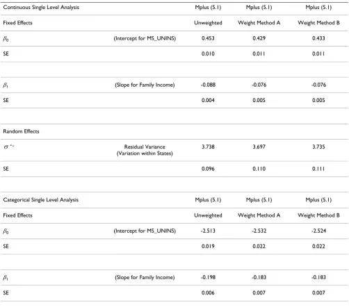
Mplus has several strengths. It has tremendous flexibility and can incorporate numerous statistical models within the MLM framework well beyond "traditional" hierarchi-cal linear and generalized linear models. One can fit factor Table 1: Single Level Continuous and Categorical outcome parameter and standard error estimates.
Continuous Single Level Analysis Mplus (5.1) Mplus (5.1) Mplus (5.1)
Fixed Effects Unweighted Weight Method A Weight Method B
β0 (Intercept for MS_UNINS) 0.453 0.429 0.433
SE 0.010 0.011 0.011
β1 (Slope for Family Income) -0.088 -0.076 -0.076
SE 0.004 0.005 0.005
Random Effects
Residual Variance (Variation within States)
3.738 3.697 3.735
SE 0.096 0.110 0.111
Categorical Single Level Analysis Mplus (5.1) Mplus (5.1) Mplus (5.1)
Fixed Effects Unweighted Weight Method A Weight Method B
β0 (Intercept for MS_UNINS) -2.513 -2.532 -2.524
SE 0.019 0.022 0.022
β1 (Slope for Family Income) -0.198 -0.183 -0.183
SE 0.006 0.007 0.007
models, latent class models, structural equation models, mixture models, latent growth curve models, and others within the MLM framework. Second, Mplus will automat-ically scale the weights for the user using each approach described here and Mplus allows analysts to specify weights scaled outside of Mplus. Third, Mplus offers a wide variety of estimators and link functions. Fourth, Mplus can handle both of the current recommended methods for analyzing subpopulations of complex survey data, the zero-weight approach and the multiple-group approach. [24]
MLwiN also incorporates several strengths. First, MLwiN can fit models with up to five levels, making it quite useful in multistage designs. Second, MLM has an easy point-and-click, windows-based user interface, which makes fit-ting MLMs easy and straightforward. Third, MLwiN incor-porates several estimators. Fourth, like Mplus, MLwiN provides an automatic weight scaling feature, and, like Mplus, it allows the user to specify weights scaled outside of MLwiN. Fifth, MLwiN has numerous features available for evaluating a model's appropriateness. And, sixth, MLwiN includes several graphical features.
Finally, GLLAMM also has some distinct advantages. Like Mplus, GLLAMM offers an astounding array of models that it can fit within the MLM framework. [30] Second, GLLAMM does allow more than two cross-sectional levels. Third, GLLAMM allows the user to specify scaled weights. Finally, GLLAMM uses full pseudo-maximum-likelihood estimation for generalized linear mixed models with any number of levels using adaptive quadrature,[10] which may result in more appropriate standard errors, especially when working with categorical outcomes. [23]
Weaknesses
Despite its strengths, Mplus has some distinct disadvan-tages. First, it can only fit two-level cross-sectional MLM models. Although one can fit a two-level MLM and use Mplus' complex data analysis feature to properly estimate standard errors for a third level, Mplus does not allow one to investigate what predicts variation at level-3. For multi-stage surveys, this may be a substantial limit. Second, rel-ative to MLwiN, Mplus offers few analytical tools for investigating model assumptions, model fit, and model diagnostics. Third, relative to MLwiN, Mplus offers few graphical tools, whether these limits outweigh its strengths will depend on the individual users needs.
MLwiN also has limits. Primarily, it cannot fit the wide variety of models that Mplus and GLLAMM can (e.g., latent class models). While MLwiN can fit some models beyond hierarchical linear and generalized linear models (e.g., multilevel confirmatory factor analyses), MLwiN does not have the full flexibility that Mplus and GLLAMM
do. For users seeking to fit extremely complex models, this may be a substantial drawback. Second, MLwiN will only automatically scale the weights using method B. And third, while MLwiN does offer several estimators (e.g., iterative generalized least squares (IGLS), restricted IGLS, and Markov chain Monte Carlo (MCMC)), it does not offer as large a range of estimators as Mplus. Again, whether these weaknesses outweigh its strengths will depend primarily on the type of analysis the user expects to conduct.
Finally, GLLAMM has some noteworthy disadvantages. First, GLLAMM has well known problems with computa-tional speed. Models that take seconds to converge in the other programs can take days (literally) to converge in GLLAMM. Aside from some minor adjustments, analysts can do little to increase GLLAMM's speed. Second, although GLLAMM has an advantage with categorical out-comes, it may be less accurate with continuous outcomes. [29,31] GLLAMM does not scale the weights for the user. Users must supply pre-scaled weights. Third, GLLAMM offers few automatic features (e.g., automatic grand or group mean centering) and diagnostic utilities. However, users familiar with STATA will find it easy to incorporate STATA commands, data manipulation, and diagnostic tools when using GLLAMM, whether these limits out-weigh its benefits will depend on the user's individual needs.
Limitations
Although these analyses generally support the use of MLM in complex survey data with design weights, some issues remain unresolved. First, a best practice for scaling weights across multiple levels has yet to be advanced. Though Asparouhov[3] and Rabe-Hesketh and Skron-dal[10] indicate that scaling level-2 weights has little prac-tical effect, more work is needed to investigate the generality of that advice, particularly in surveys with 3 or more levels. Second, complex survey designs often employ unequal probability of selection at higher levels. For example, the National Epidemiologic Survey of Alco-hol and Related Conditions[32] stratified the US into four regions. It then sampled counties within regions and peo-ple from households within counties. At both the county and household levels, unequal probability of selection occurred (e.g., some counties were more likely to be included than others). Survey organizations rarely make (or have) level-2 or beyond weights available. Some authors have suggested methods for estimating level-2 weights from level-1 weights,[17] yet more work is needed to investigate these methods' validity.
three-level model by grouping individuals according to their county of residence using data from a two-level survey that sampled people within states). However, this flexibil-ity may result in cross-classified data structures (e.g., hos-pital catchment areas overlapping states in a survey that sampled people within states). While MLM can handle cross-classified data,[16] no work has examined handling design weights in this situation.
Fourth, analysts often wish to investigate relationships within a certain subgroup. Although analysts can use interaction terms to investigate hypotheses within the specified subgroup, analysts may wish to examine a sub-group of the sample excluding other sample members entirely. For this situation, where analysts wish to investi-gate hypotheses among a specific subgroup only, no established guidelines exist regarding a best practice method for estimating MLM in complex survey data with design weights. When using complex surveys, one should include the entire sample in the analyses. This leaves the sample design structure whole and leads to proper estima-tion of variances and standard errors. However, it presents a problem when analysts would like to select a subgroup and examine a MLM for this subgroup of individuals in a sample. Analysts should not simply subset the data to the desired group of interest. [33,34] While some techniques have been suggested (e.g., zero-weighting[34] and multi-ple-group analyses[24]), the performance of these tech-niques in MLM with design weights needs further examination.
Finally, little work addresses missing data's role in MLM with design weights. It remains unclear how to best han-dle missing data within the context of MLM, complex sur-vey data, and design weights. Analysts might take a zero-weighting approach for missing data,[34] treating individ-uals with complete data as a subgroup, to address missing data. If one uses this approach, the analyst should take special care to scale the weights using the full set of weights. To evaluate the influence of missing data, ana-lysts might conduct analyses in the full sample using selected variables for which all individuals have complete data and compare those results to identical analyses con-ducted on the same variable set but using the subsample of individuals with missing data on other variables of interest. Future work should explore missing data's role and develop and test solutions to handle it.
While these limits highlight an array of outstanding issues that need investigation, they do not preclude analysts from employing MLM in complex survey data with design weights. Moreover, they demonstrate the need to choose a MLM program that allows flexibility with regard to design weights. Thus, as theory advances, software will not limit analyses.
Applied Summary Recommendations
Given the breadth of findings discussed and presented and the various strengths and weakness of each approach and software program, the reader might now wonder, "what do do in practice?" In my work, I standard approach. First, in terms of software, take the following I generally use Mplus. I do this because Mplus offers the most flexibility relative to speed. I frequently fit models that MLwiN cannot estimate (e.g., MLM multiple group structural equation models) and I rarely fit models with more than two levels (which Mplus currently cannot esti-mate). Analysts fitting the types of models discussed in this paper will generally find MLwiN more than meets their needs. Second, in terms of scaling the weights, I always fit the models using each scaling technique (meth-ods A and B). I do this to examine any inferential discrep-ancies. If I find no inferential discrepancies, I generally report the findings from method A. I do this because I fre-quently work with cluster sizes larger than n = 20 and I am interested in both point estimates and variance-covari-ance discussions. If I worked with smaller cluster sizes (n < 20) and had an interest primarily in variance-covariance estimates, I would report the results of method B. If I had an interest primarily in point estimates, I would report the results of method A. Finally, if I encountered a model I could not estimate for some reason using scaled weighted data, I would take the following approach. I would fit a simpler model using scaled weighted and unweighted data. If I did not observe a difference in the inferential conclusions across these approaches, I would then fit the more complex model using unweighted data. However, I would include a note in my reporting of the unweighted findings highlighting that I used unweighted data and that readers should interpret the results with caution.
Conclusion
to understand, describe, and improve the health of a diverse world's public health.
Competing interests
The author declares that they have no competing interests.
Authors' contributions
Using publicly available data, I worked individually, con-ducted the literature searches and summaries of previous related work, undertook the statistical analyses, wrote the manuscript, conducted all revisions, and read and approved the final manuscript.
Appendix A
A.1 Data set creationTo recreate the data used in these analyses, one needs to merge two NCHS files and add the state-level (level-2) variable. The level-1 outcome, months without insurance, is available on the NS-CSHCN "interview" dataset as CQ905. The level-1 covariate (family income) is available on the data file NCHS entitles "multiple imputation". NCHS labels the family income variable POVLEVEL_I. For these analyses, I used a single imputation, imputation 1, as suggested by Pedlow, et al. [35]
NCHS makes both datasets available at ftp://ftp.cdc.gov/ pub/Health_Statistics/NCHS/slaits_cshcn_survey/ 2005_2006/Datasets/. The level-2 covariate (proportion of families in poverty) is available at the US Census Bureau's website http://pubdb3.census.gov/macro/ 032007/pov/new46_185200_07.htm as well as Table 2. For simplicity's sake, all analyses in the current paper used individuals with complete data.
A.2 Scaling the Weights
After creating the dataset, one needs to scale the weights. In any analyses, here or otherwise, one should scale the weights before doing any other data management, as the scaled weights should be based on the entire sample of individuals with weights.
SAS Code
proc sort data = mlm;
by state;
run;
proc summary data = mlm;
by state;
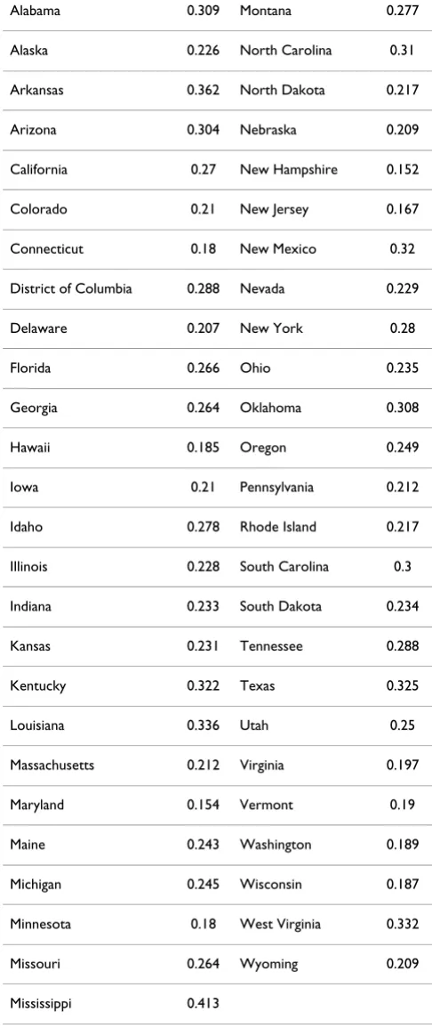
Table 2: Proportion of families in each state falling at or below the 200% poverty line.
Alabama 0.309 Montana 0.277
Alaska 0.226 North Carolina 0.31
Arkansas 0.362 North Dakota 0.217
Arizona 0.304 Nebraska 0.209
California 0.27 New Hampshire 0.152
Colorado 0.21 New Jersey 0.167
Connecticut 0.18 New Mexico 0.32
District of Columbia 0.288 Nevada 0.229
Delaware 0.207 New York 0.28
Florida 0.266 Ohio 0.235
Georgia 0.264 Oklahoma 0.308
Hawaii 0.185 Oregon 0.249
Iowa 0.21 Pennsylvania 0.212
Idaho 0.278 Rhode Island 0.217
Illinois 0.228 South Carolina 0.3
Indiana 0.233 South Dakota 0.234
Kansas 0.231 Tennessee 0.288
Kentucky 0.322 Texas 0.325
Louisiana 0.336 Utah 0.25
Massachusetts 0.212 Virginia 0.197
Maryland 0.154 Vermont 0.19
Maine 0.243 Washington 0.189
Michigan 0.245 Wisconsin 0.187
Minnesota 0.18 West Virginia 0.332
Missouri 0.264 Wyoming 0.209
var weight_i;
output out = intermediate
uss = sumsqw
sum = sumw
n = nj;
run;
data mlm;
merge mlm intermediate;
by state;
aw = weight_i/(sumw/nj);
label aw = "Method A";
bw = weight_i/(sumsqw/sumw);
label bw = "Method B";
run;
data mlm; set mlm; drop _freq_ sumsqw sumw nj _type_; run;
To update this code for other datasets, 1) replace "mlm" with the name of the dataset of interest, 2) replace "weight_i" with the level-1 weight from the dataset of interest, and 3) replace "state" with the level-2 cluster var-iable from the dataset of interest.
Stata Code
gen sqw = WEIGHT_I^2
egen sumsqw = sum(sqw), by(STATE)
egen sumw = sum(WEIGHT_I), by(STATE)
egen nj = count(IDNUMXR), by(STATE)
gen bw1 = WEIGHT_I*(sumw/sumsqw)
gen aw1 = WEIGHT_I*(nj/sumw)
To update the Stata code for other datasets, 1) read the dataset of interest into memory, 2) replace "weight_i" with tje level-1 weight from the dataset of interest, 3) replace "state" with the level-2 cluster variable from the dataset of interest, and, 4) replace "idnumxr" with the level-1 id variable from the dataset of interest.
Appendix B: Equations for Scaling the Weights
B.1 Method AB.2 Method B
For both, represents the scaled weight for individual i
in cluster j, wij the unscaled weight for individual i in clus-ter j, and nj the number of sample units in cluster j .
Appendix C: Traditional MLM Equations
C.1 Continuous ModelsC.1.1 Unconditional model
C.1.2 Level-1 Predictor Only (Fixed Effect)
C.1.3 Level-1 Predictor Only (Fixed and Random Effects)
C.1.4 Level-2 Predictor Only (Fixed Effect)
C.1.5 Level-1 and Level-2 Predictors, No Cross-Level Interaction
C.1.6 Level-1, Level-2, and Cross-Level Interaction
w w n j
wij i ij ij ∗ = ∑ ⎛ ⎝ ⎜ ⎜ ⎞ ⎠ ⎟ ⎟
w w iwij
wij i ij ij ∗ = ∑ ∑ ⎛ ⎝ ⎜ ⎜ ⎜ ⎞ ⎠ ⎟ ⎟ ⎟ 2
wij∗
Months Uninsured e
u
ij j ij
j j _ = + = + β β β 0
0 0 0
Months Uninsured Family Income e
u
ij j j ij ij
j j _ = + + = + β β β β 0 1
0 0 0
Months Uninsured Family Income e
u
ij j j ij ij
j j j _ = + + = + β β β β β 0 1
0 0 0
1 ==β1+u1j
Months Uninsured State Poverty e
u
ij j j ij
j j _ = + + = + β β β β 0 1
0 0 0
Months Uninsured_ ij=β0j+β1jFamily Incomeij+β2State Povertyj++
= + = + e u u ij j j j j β β β β
0 0 0
1 1 1
Months Uninsured
Family Income State Poverty
ij
j j ij j
_ =
+ +
β0 β1 β2 ++ × +
= + = + β β β β β 3
0 0 0
1 1 1
Family Income State Poverty e
u u
ij j ij j j
C.2 Categorical Models
C.2.1 Unconditional model
C.2.2 Level-1 Predictor Only (Fixed Effect)
C.2.3 Level-1 Predictor Only (Fixed and Random Effects)
C.2.4 Level-2 Predictor Only
C.2.5 Level-1 and Level-2 Predictors, No Cross-Level Interaction
C.2.6 Level-1, Level-2, and Cross-Level Interaction
C.3 Variance Components
In all models,
= The variance of eij (i.e., the residual variance within
states).
= The variance of u0j (i.e., the variance in the intercepts between states).
= The variance of u1j (i.e., the variance in slopes between states).
σ01 = COV(u0j, u1j) (i.e., the covariance between the inter-cepts and slopes).
Appendix D: Original Weights
This appendix briefly summarizes the methodology used to weight the 2005–2006 NS-CSHCN. Generally, the weighting scheme for the sample involved the steps below. Here, I only describe the base weights. Readers interested in more detail should consult Blumberg et al. [27].
1. Compute base sampling weight.
2. Adjustment for nonresolution of released telephone numbers.
3. Adjustment for incomplete age-eligibility screener.
4. Adjustment for incomplete CSHSCN Screener.
5. Adjustment for multiple telephone lines.
6. Raking adjustment of household weights.
7. Raking adjustment of child screener weights.
8. Adjustment for subsampling of CSHCN.
9. Adjustment for nonresponse to the CSHCN inter-view.
10. Raking of adjustment of the nonresponse-adjusted CSHCN interview weights.
The base weight equals the reciprocal of the selection probability of the kth telephone number:
πk = probability of selecting the kth telephone number in the estimation area.
nq = sample size in quarter q in the estimation area. Uninsured u ij ij ij j j j ~ ( , ) ( ) Binomial logit 1 0
0 0 0
π π β β β = = + Uninsured Family Income ij ij
ij j j
~ ( , ) ( ) Binomial logit 1 0 1 π π =β +β ββ β
β10jj β10 10jj
u u = + = + Uninsured Family Income ij ij
ij j j
~ ( , ) ( ) Binomial logit 1 0 1 π π =β +β ββ β
β β
0 0 0
1 1 1
j j j j u u = + = + Uninsured State Poverty ij ij
ij j j
~ ( , ) ( ) Binomial logit 1 0 1 π
π =β +β jj
j u j
β0 =β0+ 0
Uninsured
Family Income
ij ij
ij j j
~ ( , ) ( ) Binomial logit 1 0 1 π
π =β +β ++
= + = + β β β β β 2
0 0 0
1 1 1
State Poverty u u j j j j j Uninsured Family Income ij ij
ij j j
~ ( , ) ( ) Binomial logit 1 0 1 p
p =b +b ++ + ×
= +
b b
b b
2 3
0 0 0
State Poverty Family Income State Poverty u
j j
j jj
j uj
b1 =b1+ 1
σe2
σ02
σ12
Nq = total telephone numbers on the sampling frame in quarter q in the estimation area.
Following computation of the base weight, several adjust-ments followed. Blumberg, et al.,[27] describe these adjustments in detail.
Additional material
Acknowledgements
I would like to the US Health Resources and Services Administration, Maternal and Child Health Bureau and the US Centers for Disease Control and Prevention, National Center for Health Statistics for making the data publicly available. I would also like to thank Tara J. Carle and Margaret Carle whose unending support and thoughtful comments make my work possible. I am also grateful to Stephen J. Blumberg for his collegial support and his dedication to bridging gaps between advanced methodologies and applica-tions in order to improve children's health. Finally, I would like to thank all four reviewers. Their tireless work and insightful comments vastly improved the original manuscript.
References
1. Asparouhov T: General Multi-Level Modeling with Sampling Weights. Communications in statistics. Theory and methods 2006,
35(3):439-460.
2. Asparouhov T: Sampling weights in latent variable modeling.
Structural equation modeling 2005, 12(3):411-434.
3. Asparouhov T: Scaling of Sampling Weights For Two Level Models in Mplus 4.2 CA: Muthén and Muthén; 2008.
4. Chambers RL, Skinner CJ, (Eds.): Analysis of Survey Data Chichester: Wiley; 2003.
5. Graubard BI, Korn EL: Modeling the sampling design in the analysis of health surveys. Statistical Methods in Medical Research
1996, 5:263-281.
6. Longford NT: Model-based variance estimation in surveys with stratified clustered designs. Australian Journal of Statistics
1996, 38:333-352.
7. Longford NT: Models for Uncertainty in Educational Testing New York: Springer; 1995.
8. Longford NT: Model-based methods for analysis of data from 1990 NAEP Trial State Assessment. Washington, DC: National Center for Education Statistics; 1995.
9. Pfeffermann D, Skinner CJ, Holmes DJ, Goldstein H, Rasbash J:
Weighting for unequal selection probabilities in multilevel models. Journal of the Royal Statistical Society. Series B, Statistical meth-odology 1998, 60:23-40.
10. Rabe-Hesketh S, Skrondal A: Multilevel modelling of complex survey data. Journal of the Royal Statistical Society. Series A, Statistics in society 2006, 169:805-827.
11. Merlo J: Multilevel analytical approaches in social epidemiol-ogy: Measures of health variation compared with traditional measures of association. Journal of Epidemiology & Community Health 2003, 57(8):550-551.
12. Merlo J, Chaix B, Yang M, Lynch J, Rastam L: A brief conceptual tutorial on multilevel analysis in social epidemiology: Inter-preting neighbourhood differences and the effect of neigh-bourhood characteristics on individual health. Journal of Epidemiology & Community Health 2005, 59(12):1022-1028. 13. Merlo J, Yang M, Chaix B, Lynch J, Rastam L: A brief conceptual
tutorial on multilevel analysis in social epidemiology: Inves-tigating contextual phenomena in different groups of people.
Journal of Epidemiology & Community Health 2005, 59(9):729-736. 14. Merlo J, Chaix B, Ohlsson H, Beckman A, Johnell K, Hjerpe P, Rastam
L, Larsen K: A brief conceptual tutorial of multilevel analysis in social epidemiology: Using measures of clustering in mul-tilevel logistic regression to investigate contextual phenom-ena. Journal of Epidemiology & Community Health 2006,
60(4):290-297.
15. Pickett KE, Pearl M: Multilevel analyses of neighbourhood soci-oeconomic context and health outcomes: A critical review.
Journal of Epidemiology & Community Health 2001, 55(2):111-122. 16. Raudenbush SW, Bryk AS: Hierarchical linear models: applications and
data analysis methods Thousand Oaks, CA: Sage; 2002.
17. Goldstein H: Multilevel statistical models 3rd edition. London: Hodder Arnold; 2003.
18. Research Triangle Institute: SUDAAN User's Manual: Release 8.0. Research Triangle Park, NC: Research Triangle Institute; 2002. 19. Skinner CJ: Domain means, regression and multivariate anal-ysis. In Analysis of complex surveys Edited by: Skinner CJ, Holt D, Smith TM. Chichester: Wiley; 1989:59-87.
20. Grilli L, Pratesi M: Weighted estimation in multilevel ordinal and binary models in the presence of informative sampling designs. Survey Methodology 2004, 30:93-103.
21. Muthén LK, Muthén BO: Mplus User's Guide Fourth edition. Los Ange-les, CA: Muthén & Muthén; 1998.
22. Rasbash J, Steele F, Browne WJ, Prosser B: A user's guide to MLwiN version 2.0. University of Bristol UK: Centre for Multilevel Modelling; 2005.
23. Rabe-Hesketh S, Skrondal A, Pickles A: GLLAMM Manual: Berkeley, CA: U. C. Berkeley Division of Biostatistics Working Paper Series 2004. 24. Asparouhov T, Muthén B: Multilevel modeling of complex
sur-vey data. Proceedings of the Joint Statistical Meeting ASA section on Sur-vey Research Methods 2006:2718-2726.
25. Raudenbush SW, Bryk T, Congdon R: HLM 6 Chicago: Scientific Soft-ware International; 2006.
26. SAS Institute: SAS/STAT 9.1, User's Guide Cary, NC: SAS Institute Inc; 2004.
27. Blumberg SJ, Welch EM, Chowdhury SR, Upchurch HL, Parker EK, Skalland BJ: Design and operation of the National Survey of Children With Special Health Care Needs, 2005–2006. Vital Health Statistics 2008, 45(1):1-132.
28. Singer JD, Willett JB: Applied Longitudinal Data Analysis: Modeling Change and Event Occurrence NY, NY: Oxford University Press; 2003. 29. Rabe-Hesketh S, Skrondal A, Pickles A: Maximum likelihood esti-mation of limited and discrete dependent variable models with nested random effects. Journal of Econometrics 2005,
128:301-323.
30. Rabe-Hesketh S, Skrondal A, Pickles A: Generalized multilevel structural equation modeling. Psychometrika 2004,
69(2):167-190.
Additional file 1
Continuous outcome parameter and standard error estimates across level-1, level-2, combined-level models, weight scaling methods, and software programs. The data provided present the multilevel results across continuous models, weight scaling methods, and software pro-grams.
Click here for file
[http://www.biomedcentral.com/content/supplementary/1471-2288-9-49-S1.pdf]
Additional file 2
Categorical outcome parameter and standard error estimates across level-1, level-2, combined-level models, weight scaling methods, and software programs (Mplus estimates a threshold rather than an intercept. These differ only in sign. [21]For presentation, I converted the thresh-old to a slope). The data provided present the multilevel results across cat-egorical models, weight scaling methods, and software programs. Click here for file
Publish with BioMed Central and every scientist can read your work free of charge
"BioMed Central will be the most significant development for disseminating the results of biomedical researc h in our lifetime."
Sir Paul Nurse, Cancer Research UK
Your research papers will be:
available free of charge to the entire biomedical community
peer reviewed and published immediately upon acceptance
cited in PubMed and archived on PubMed Central
yours — you keep the copyright
Submit your manuscript here:
http://www.biomedcentral.com/info/publishing_adv.asp
BioMedcentral 31. Rabe-Hesketh S, Skrondal A: Multilevel and Longitudinal Modeling using
Stata College Station: Stata; 2005.
32. Grant BF, Kaplan K, Shepard J, Moore T: Source and Accuracy State-ment for Wave 1 of the 2001–2002 National Epidemiologic Survey on Alcohol and Related Conditions Bethesda MD: National Institute on Alcohol Abuse and Alcoholism; 2003.
33. Korn EL, Graubard BI: Analysis of Health Surveys New York: Wiley; 1999.
34. Korn E, Graubard BI: Estimating variance components by using survey data. Journal of the Royal Statistical Society. Series B, Statistical methodology 2003, 65:175-190.
35. Pedlow S, Luke JV, Blumberg SJ: Multiple Imputation of Missing Household Poverty Level Values from the National Survey of Children with Special Health Care Needs, 2001, and the National Survey of Children's Health, 2003. 2007 [http:// www.cdc.gov/nchs/about/major/slaits/
publications_and_presentations.htm]. National Center for Health Statistics Retrieved February 05, 2009
Pre-publication history
The pre-publication history for this paper can be accessed here: