M E T H O D O L O G Y
Open Access
Using the value of Lin
’
s concordance correlation
coefficient as a criterion for efficient estimation of
areas of leaves of eelgrass from noisy digital
images
Héctor Echavarría-Heras
1*, Cecilia Leal-Ramírez
1, Enrique Villa-Diharce
2and Oscar Castillo
3Abstract
Background:Eelgrass is a cosmopolitan seagrass species that provides important ecological services in coastal and near-shore environments. Despite its relevance, loss of eelgrass habitats is noted worldwide. Restoration by replanting plays an important role, and accurate measurements of the standing crop and productivity of transplants are important for evaluating restoration of the ecological functions of natural populations. Traditional assessments are destructive, and although they do not harm natural populations, in transplants the destruction of shoots might cause undesirable alterations. Non-destructive assessments of the aforementioned variables are obtained through allometric proxies expressed in terms of measurements of the lengths or areas of leaves. Digital imagery could produce measurements of leaf attributes without the removal of shoots, but sediment attachments, damage infringed by drag forces or humidity contents induce noise-effects, reducing precision. Available techniques for dealing with noise caused by humidity contents on leaves use the concepts of adjacency, vicinity, connectivity and tolerance of similarity between pixels. Selection of an interval of tolerance of similarity for efficient measurements requires extended computational routines with tied statistical inferences making concomitant tasks complicated and time consuming. The present approach proposes a simplified and cost-effective alternative, and also a general tool aimed to deal with any sort of noise modifying eelgrass leaves images. Moreover, this selection criterion relies only on a single statistics; the calculation of the maximum value of the Concordance Correlation Coefficient for reproducibility of observed areas of leaves through proxies obtained from digital images.
Results:Available data reveals that the present method delivers simplified, consistent estimations of areas of eelgrass leaves taken from noisy digital images. Moreover, the proposed procedure is robust because both the optimal interval of tolerance of similarity and the reproducibility of observed leaf areas through digital image surrogates were
independent of sample size.
Conclusion:The present method provides simplified, unbiased and non-destructive measurements of eelgrass leaf area. These measurements, in conjunction with allometric methods, can predict the dynamics of eelgrass biomass and leaf growth through indirect techniques, reducing the destructive effect of sampling, fundamental to the evaluation of eelgrass restoration projects thereby contributing to the conservation of this important seagrass species.
Keywords:Eelgrass leaf, Area estimations, Noisy digital images selection criterion, Concordance correlation coefficient
* Correspondence:[email protected]
1Centro de Investigación Científica y de Estudios Superiores de Ensenada,
Carretera Ensenada-Tijuana No. 3918, Zona Playitas, Apdo. Postal 360, Código Postal 22860 Ensenada, B C, México
Full list of author information is available at the end of the article
Background
Seagrass meadows are highly productive plant communi-ties that grant valuable ecological services in estuaries and near-shore environments worldwide. Seagrasses provide food and shelter for a myriad of economically and eco-logically valued marine organisms [1-3], play an important role in nutrient cycling [4,5], favor the stabilization of the shoreline as roots and rhizomes compact the substrate, preventing erosion [6,7], participate in the foundation of the detrital food web [8], and play also, a fundamental role in carbon sequestration [9]. Eelgrass (Zostera marina L.) is particularly relevant not only because it is the dominant seagrass species along the coasts of both the North Pacific and North Atlantic [10], but also, because eelgrass com-munities have been traditionally recognized as among the richest and most varied in the abundance of sea life [11]. Indeed, this cosmopolitan macrophyte was found to pro-duce up to 64% of the total primary production of an estu-arine system [12].
The forcing of Zostera marina dynamics by environ-mental variables is well documented in the literature [13-18]. Light availability, temperature, and dissolved nu-trients are the most important variables for explaining the observed variability [18,19]. But even when light and nutrients are not limiting, temperatures ranging above the upper limit tolerated by eelgrass can provoke severe negative effects on its growth [20]. Indeed, the onset of warm ENSO events has been shown to dramatically di-minish eelgrass growth [20]. Therefore, the productivity of Zostera marinapopulations could be diminished by global climate change, which is expected to result in warming and rising seas, thereby reducing the availability of both light and nutrients underwater [21]. Another concern for the health of eelgrass populations pertains to increasing deleterious anthropogenic influences. The loss of eelgrass habitat has been noted worldwide, with major losses in the past few decades [22-25]. Within restoration strat-egies, replanting plays an important role [26-28]. The monitoring of these efforts is fundamental for the evalu-ation of the effectiveness of restorevalu-ation of functions and values of natural populations. Accurate measurements of the standing crop and productivity of transplanted popula-tions at a given time constitute an important input for evaluating the restoration of the ecological functions and values of natural populations. Although traditional assess-ment methods do not cause damage to natural popula-tions, their invasive nature could significantly alter the development of transplanted populations. Echavarria-Heras et al. [29] and Echavarria-Echavarria-Heras et al. [30] propose allometric methods that reduce eelgrass biomass and leaf growth rate estimations to measurements of leaf length or area. Besides, the use of digital imagery could provide leaf area estimations which avoid invasive effects. But in some cases noise effects could lead to misidentification of
pixels placed on the peripheral contour of leaves images (see Figure 1). This could spread uncertainty on leaf area estimations that ultimately could render imprecise allo-metric projections of biomass and leaf growth rates. Therefore, for accurateness we must rely on an image se-lection method that produces an unambiguous identifica-tion of the sequence of pixels that form the peripheral contours of digitalized eelgrass leaves. In order to achieve this task, there are techniques developed on the basis of the concepts of adjacency, vicinity, connectivity and toler-ance of similarity between pixels (see Appendix). Using this framework Leal-Ramirez and Echavarria-Heras [31] introduced a direct comparison method aimed to discrim-inate the interval of tolerance of similarity that produces the most accurate estimations of length, width or area of eelgrass leaves from digital images with noise induced by humidity contents. For a given interval of tolerance of similarity, the process initially identifies the peripheral contour of the images of leaves and then measures the concomitant lengths widths and areas. Next, individual deviations between leaf area measurements taken from images and those obtained directly from leaves are used to produce statistics aimed to obtain the proportions of leaves for which image assessments underestimate or overestimate observed values. The ratio of these propor-tions defines a selection index whose smallest value pro-vides criterion for choosing the interval of tolerance of similarity that yields the most accurate image related mea-surements. The implementation of the direct comparison method uses lengthy computational stages that include various statistical inferences on deviations between ob-served an image obtained leaf areas. In this contribution, we present an alternative criterion for the selection of the named interval of tolerance of similarity. The present pro-cedure called the concordance correlation method; is sim-pler to implement than the direct comparison method. It only requires calculating the values of the Concordance Correlation Coefficient (CCC) for the reproducibility of observed leaf areas through proxies obtained from corre-sponding images. The present criterion proposes the use of the interval of tolerance of similarity that yields the maximum value of the aforementioned CCC for consist-ent digital image estimations of eelgrass leaves areas. Our results show that on spite of its simplicity the present se-lection criterion yields highly reliable levels of accuracy.
In section two, we present a brief review of the direct comparison method. Section three formally explains the present concordance correlation method. Section four de-scribes the results of this study and discusses the advan-tages and possible drawbacks of the present approach.
The Direct Comparison Method (DCM)
Echavarria-Heras [31]. Initially, the DCM chooses a positive integernand uses it to fix a tolerance levelq= (lmax/n), being lmax the maximum observed leaf length.
This yields a covering for the range [0,lmax] by a
collec-tion of ndisjoint intervals of the form Ik= [q(k−1),qk),
with 1≤k≤ n. Subsequently, for each value of the index k the procedure identifies the group Gk(l) of nk leaves
whose lengths are contained inIk. An index j such that
1≤j≤ nklabels leaves inGk(l) while the symbols lkoj, hkoj and akoj denote respectively the straight length, width and area of thejth leaf inGk(l). Particularly, estimations
ak
oj of the leaf areas inGk(l) can be obtained by using the
length times width proxy [32]. Digital images of leaves in theGk(l) groups are processed by a specified color format
with a number Cmaxof colors and via intervals of
toler-ance of similarity ST(r) = [0,r], being r, 0≤r≤Cmax−1,
the number of different tonalities used for pixel identifica-tion. By keeping ST(r) fixed, a routine selects a starting point within the image of thejth leaf inGk(l) and detects
all adjacent pixels falling within the selected interval of tolerance of similarity ST(r). This task which is achieved using equations (A1), (A2) and (A3) identifies the periph-eral contour of the leaf image, and allows the measure-ments of the concomitant proxies for the length lkdjð Þr ,
width hkdjð Þr and area akdjð Þr of the leaf. Afterwards the method obtains the deviations for leaf length ek
ljð Þr , width ek
hjð Þr and area ekajð Þr , given by: eljkð Þ ¼r lkoj−lkdjð Þr ,
ek
hj¼hkoj−hkdjð Þr ,andekajð Þ ¼r akoj−akdjð Þr . This produces re-spective average deviation values taken over groupsGk(l).
These are denoted by means ofδklð Þr , δhkð Þr , δkað Þr , their corresponding averages taken over the whole collection of groupsGk(l) by means ofδlð Þr ,δhð Þr ,δað Þr and the asso-ciated standard deviations throughσδl(r),σδh(r) andσal(r)
respectively. Then, for each range of similarityST(r), the technique identifies the leaves satisfying the conditions
δhð Þr ≥0; ð1Þ
δlð Þr≥0; ð2Þ
δlð Þr−σδlð Þr ≤δklð Þr≤δlð Þ þr σδl ð Þr ; ð3Þ
δhð Þr −σδhð Þr ≤δhð Þr ≤δhð Þ þr σδhð Þr ð4Þ
and
ekajð Þr ≥0 ð5Þ
and use their area values ak
djð Þr to calculate λa(r), which stands for the proportion of images of leaves for which
ad produces consistent estimations of observed leaf areas a0. This proportion is calculated according to the formula,
λað Þ ¼r
Xn k¼1
Xnk j¼1½a
k
djð Þ jr leaves inGkð Þl that comply
with conditions 1ð Þthrough 5ð Þ
Xn k¼1
Xnk j¼1a
k oj
ð6Þ
Then the method obtains the proportion βa(r) of
im-ages of leaves for which ad estimations overestimates
observed leaf areas ao which is calculated through βa
(r) = 1− λa(r), and use λa(r) and βa(r) to calculate the
value of the image selection index IS(r), formally de-fined by
IS rð Þ ¼βað Þr =λað Þr ð7Þ
Finally, the DCM proposes the use of the ST(r) inter-val producing the smallest inter-value ofIS(r) for reliable esti-mation of the areas of leaves of eelgrass using images whose peripheral contour is distorted by noise induced by humidity contents.
The Concordance Correlation Method (CCM)
The Concordance Correlation Coefficient symbolized by mean of ρ [33,34] is used to determine reproducibility, as it measures the agreement between the variables x and y by appraising the extent to which they fall on the 45° line through the origin. Its numerical value is repre-sented in terms of the ratio of the expected orthogonal squared distance from the diagonaly=xto the expected
Figure 1A digital image of aZostera marinaleaf. a)An image ofa Zostera marinaleaf exhibiting the typical belted shape. Related area is
orthogonal squared distance from the diagonal y=x as-suming independency. The value of ρ, is commonly used to assess how well a new set of observationsy reproduce an original setx. Whenρis computed on am-length data set (i.e., two vectors (x1,x2,⋯,xm) and (y1,y2,⋯,ym) the
resulting statistics is denoted by means of^ρand calculated through
^
ρ¼ 2sxy
s2
x þs2yþ ðxþyÞ
2 ; ð8Þ
being
x¼ 1 m
Xm
j¼1
xj ð9Þ
s2
x ¼ 1
m Xm
j¼1 xj−x
2
ð10Þ
and
sxy¼ 1
m Xm
j¼1 xj−x
yj−y
ð11Þ
In the present work the value ofρ^will provide a criter-ion for the incumbent digital image selectcriter-ion process. The linked CCM does not require the sorting of ob-served leaf lengths into theGk(l) groups of the DCM. As
it is done in the DCM, in the present CCM, the digital images of sampled leaves are primarily processed by a specified color format with a numberCmaxof colors and
using intervals of tolerance of similarity ST (r) = [0,r] with 0≤r≤Cmax−1. Again by keeping ST(r) fixed and
within the jth leaf image, a routine selects a starting point, and using Eqs. (A1), (A2) and (A3) detects all ad-jacent pixels connected within the realm of the desig-nated interval of tolerance of similarity ST(r). This device identifies the peripheral contour of the leaf image allowing associated measurements of length ldj(r) and
widthhdj(r) whose product for 1≤j≤m, yields image
es-timated leaf areasadj(r). Instead of performing the
statis-tical steps required to calculate IS(r), simply for r fixed in equations (9), (10) and (11) we make xjstand for
ob-served leaf area measurements (a01,a02,⋯,a0m) and let
y match digital image produced estimations (ad0(r),ad1 (r),⋯,adm(r)). Then equation (8) yields the resulting
value of the Concordance Correlation Coefficient. In the present settings this will be denoted through by means of the symbol ^ρð Þr to emphasize its dependence on r, that is, changing ST(r) produces different pairs of ob-served and image calculated leaf areas (a0j ,adj(r)), 1≤
j≤m, as well as different values of the associated ρ^ð Þr . After all values of r in the chosen color format are exhausted, we select the tolerance of similarity interval ST(r) that produces the highest value for ^ρð Þr for
efficient estimation of eelgrass leaves area from digital im-ages with noise related to environmental factors.
Results and discussion
For the purposes of the present study, we used a data set obtained by randomly sampling 5 shoots biweekly from January through December 2009 in a Zostera marina field at Punta Banda estuary, a shallow coastal lagoon located near Ensenada, Baja California, Mexico (31° 43–46 N and 116° 37–40 W). For each sampled leaf, a millimeter ruler was used to obtain leaf length mea-surements lo to the nearest 1/10mm taken as the
dis-tance from the top of the sheath to the leaf tip. Meanwhile, observed leaf width ho was measured at a
point halfway between the top of the sheath and the tip [32]. Observed leaf area estimationsaowere calculated by
means of length times width proxyao=lo⋅ho.
We obtained lmax= 460 mm. For the data grouping
required by the DCM we choose n= 46 so we
ac-quired q= 10 mm, and for the interval [0,lmax] we
formed a partition P460
0 of disjoint intervals Ik of the
form Ik= {l | q(k−1)≤l<qk}, with 1≤k≤46. Hence,
for each value of the index k, we formed a group Gk
(l) containing leaves with sizes varying in the interval Ik. Longer and older leaves displayed darker tonalities
than younger and shorter ones, but leaves with lengths varying on a given partition intervalIkdisplayed a similar
color distribution. For some of the partition intervals there was at most one leaf with length placed in the linked vari-ation range. Therefore, these groups are not taken into ac-count because they do not provide information for the statistical analysis.
According to the DCM, for each leaf belonging to the group Gk(l) we obtained its digital image. For dealing
out with all these individual images we selected an RGB color format with a numberCmaxof 256 colors. For
pro-cessing each one of the available leaves images, we choose different tolerance of similarity levels ST(r) = [0,r] with the upper bound rsatisfying 0≤r≤Cmax−1. Then for a
givenST(r) range, we selected a starting point inside the considered leaf image, and identified using equations (A1), (A2) and (A3) all adjacent pixels falling within the named similarity rangeST(r). This recognizes the outer contour of the digital blade, and produce concomitant leaf width, length and area estimations. The next step in the DCM concerns the calculation of the selection indexIS(r) which depends on the value of theλa(r) statistics. But according
to equation (6) obtaining the value ofλa(r) requires
count-ing the number of leaves in each groupGk(l), that comply
can be expected to be imprecise. This is handily clarified by Figure 2, produced usingr= 10 and that shows a sys-tematic tendency for average length deviations δklð Þr de-pending on group indexk.As a result we can observe a large number of δklð Þr values lying above the δlð Þ þr σδl
r
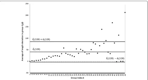
ð Þ and beyond the δlð Þr −σδlð Þr thresholds in inequality (3). The bigger the value ofr, the greater the number of color tonalities included in the intervalST(r) and precision in image contour identification improves. This is observed in Figure 3, produced using r= 128 and which does not display the above quoted systematic tendency, but a re-duced number of groups of leaves with average length de-viations δklð Þr lying outside the interval bounded by
δlð Þ þr σδlð Þr and δlð Þr −σδlð Þr . Consequently, for small values ofrwe can expect reduced values ofλa(r) and as a
result according to equation (7) large values ofIS(r). Add-itionally, when the interval of tolerance of similarity be-comes wider, smaller values of IS(r) can be expected. In fact, as shown in Figure 4, the DCM captures this effect in a consistent way, with small values of rleading to large values for the selection indexIS(r). Moreover, through the interval 1≤r< 128, IS(r), decreases reaching a minimum value of 0.91, attained at r= 128. Meanwhile, for r≥128, the values of the selection index IS(r) steadily increased towards a value of 1.84, attained atr= 255. Therefore, ac-cording to the DCM selection criterion ST(128) must be
chosen for efficient estimation of areas of eelgrass leaves using images with noise induced by humidity contents.
Now for the CCM, since a small value of r fails to recognize some pixels in the digital image, we might ex-pect a low reproducibility of directly obtained measure-ments (a01,a02,⋯,a0m) by means of digitally obtained
proxies (ad0(r),ad1(r),⋯,adm(r)). This is indeed shown
in Figure 5. Moreover , the larger the value of r, the greater the number of color tonalities included in the interval ST(r), as a result exactness in image contour identification increases, and reproducibility improves, this explaining why Figure 5 shows increasing values of ^
ρð Þr through the interval 1≤r< 128. Moreover, through the domain 128≤r< 178 the values of^ρð Þr are maintained within a plateau of slight variation around^ρð128Þ ¼0:90, but for 178≤r≤255,^ρð Þr decreases dropping to a value of 0.8464, attained atr= 255. Thenceforth, intervals of toler-ance of similarity, wider thanST(128) do not improve re-producibility of observed values of leaves areas by means of their image obtained surrogates. Thus, for the sake of accuracy and simplicity,ST(128) should be used for image selection when noise due to environmental factors is present and efficient estimations of eelgrass leaf area taken from these images are required.
In order to assess robustness of the CCM, we per-formed a resampling experiment. We chose a sample size indexp= 1, 2,…, 8 then for each value ofpa sets(p)
Figure 2The effect of similarity indexr= 10 on average deviationsδklð Þr.Forr= 10 a regular tendency ofδklð Þr depending on group indexk
of samples of size 100peach were uniformly drawn from the (a01,a02,⋯,a0m) population. Next, we selected one
of the s(p) samples, for each value of r through the interval 1≤r≤255, we designated the matching areas obtained from digital images and calculated the concomi-tant Concordance Correlation Coefficient values^ρð Þr . We recorded the value ofr at which the maximum for ρ^ð Þr was attained for the selected sample. We repeated this procedure for all the samples in the sets(p) and then aver-aged the obtained r values for maximum ^ρð Þr . Figure 6 displays the obtained averages for the different values of the sample size indexp. The maximum values of^ρð Þr per sample were also averaged over the s(p) sets. These last average values are shown in Figure 6. The results of this study show that the optimal interval of tolerance of simi-larity, as well as, the reproducibility of observed leaf areas by means of their digital image surrogates can be consid-ered independent of sample size. Therefore, the CCM can be regarded as a robust procedure.
According to our results, both methods sustain the same conclusion regarding the choosing of ST(128) on behalf of accuracy. However, in comparison to the com-plicated multi-stage procedures of the DCM, using ρ^ð Þr values provide a direct and simpler criterion for choos-ing an interval of tolerance of similarityST(r) for reliable digital image related assessments of eelgrass leaf area under the specified noise effects. But the main advantage
of the CCM resides on the fact that it allows a straightfor-ward interpretation of the addressed digital image selec-tion procedures in terms of a measure of reproducibility. Indeed the plateau in ^ρð Þr values linked to the domain 128≤r≤178, and the subsequent decreasing mode associ-ated tor≥178 shown in Figure 5 indicate that intervals of tolerance of similarity wider thanST( 128) will fail to im-prove reproducibility of observed values of leaf area by means of their image produced proxies. In other words for r≥128, ST(r) includes more tonalities than those contained within the real image, thereby favoring the incorporation of spurious entries appearing beyond its peripheral contour and within the framing of the image. Thus including more color tonalities than necessary in the image processing task could not grant a gain in accuracy, but instead, depending on the severity of the noise effects (Figure 1), and on the size of the framing enclosing the peripheral contour of the image (Figure 1), more spurious pixels could be taken in to account by the image process-ing devise, which could lead to increased miscalculation of leaf area obtained from images. Meanwhile, our analysis confirms that when noise induced into images by the hu-midity contents of the leaves reduces the accuracy of esti-mations of the associated areas we could use a RGB color format, anST( 128) interval of tolerance of similarity and equations (A1), (A2) and (A3) to identify the peripheral contour of leaves images for optimal reproducibility. Figure 3The effect of similarity indexr= 128 on average deviationsδklð Þr.Forr= 128 the regular tendency of increasingδklð Þr values
shown figure 2 is no longer observed and a reduced number ofδklð Þr values lying outside the interval bounded byδlð Þ þr σδlð Þr andδlð Þr −σδl
r
Conclusions
The results of the present digital image selection proced-ure provide simple, unbiased and non-destructive mea-surements of eelgrass leaf area. These meamea-surements in conjunction with allometric methods [35] can predict the dynamics of biomass and leaf growth through indir-ect techniques, reducing the destructive effindir-ect of sam-pling and simplifying time consuming methods in the laboratory [36]. Nevertheless, it is worth to emphasize, that leaves removed from a shoot readily begin to lose water and degrade, so changes in shape may occur [37]. Therefore, even though humidity contents could cer-tainly induce noise effects, an efficient digitalizing of a Zostera marina blade requires the maintenance of an optimal humidity for increased image fidelity. By taking this into account we can assert that the apparent similar-ity of values of ρ^ð Þr linked to the interval 128≤r≤178 could not be exhibited as a weakness of the CCM, that is, the plateau shown in Figure 5 does not associate
to vagueness in the imbedded selection criteria. In-deed in this study both the preparation of lives before digitalization procedures and the framing used to bound the area surrounding the peripheral contour of the digital leaves was effective (1) for reducing inconsistencies attrib-utable to a biased mapping of leaf shape into images, (2) by lessening bias due to the inclusion of spurious entries linked to noise into images and (3) because the framing size used in the present identification procedure further limited the participation of spurious entries in image pro-cessing tasks. Therefore, r= 128 (that is, the entrance threshold for the plateau of maximum ρ^ð Þr values in Figure 5) includes the required number of different tonal-ities for the processing of the present set of images and we choose it for a consistent estimation of the pertinent leaf area. Although, in the present settings the aforementioned bias reduction practices explain why values of r beyond r= 128 sustain the same selection criterion, usingr≥128 could lead to extended time consuming computational
Figure 4The behavior of theIS(r)selection index through the interval 1≤r< 255.For small values ofrthe interval of tolerance of similarity
ST(r) does not include the necessary tonalities that the image identification procedure requires. Therefore identification of pixels within an image can be expected to be imprecise. Consequently reduced values ofλa(r), will be expected, which lead to large values of theIS(r) selection index.
procedures, because more than necessary tonalities will be included in the identification undertaking. It is also worth to highlight that in further applications, before the CCM could provide consistent results, care should be taken in order to ensure that the handling of samples be performed
in an efficient way for reducing bias in the overall image selection procedures. Indeed we could anticipate that in settings where points (1) through (3) above are disre-garded, the inherent bias could seriously reduce reprodu-cibility. Nevertheless, this could not be exhibited as a
Figure 5The behavior of the concordance correlation coefficientρ^
ðrÞ, through the interval 1≤r< 255.Increasing values of^ρð Þr through
the interval 1≤r< 128 are displayed. This means that the wider the interval of similarityST(r) the greater the reproducibility of observed leaf areas by image proxies becomes. Interestingly through the domain 128≤r< 178 values ofρ^ð Þr are maintained within a plateau of slight variation around^ρð128Þ ¼0:90. Afterwards, for 178≤r≤255 values of^ρð Þr decrease slightly until^ρð Þr drops to a value of 0.8464 attained atr= 255. Then for values ofrlarger thanr= 128 reproducibility is not improved and coinciding with the criterion in the DCM for the present data, both an RGB color format and theST(128) interval of tolerance of similarity could be used for image selection when noise due to humidity contents is present and efficient estimations of eelgrass leaf area taken from these images is required.
Figure 6Dependence of both the value ofrfor maximumρ^ð
rÞand the maximum value ofρ^ð
rÞitself on sample size.For each value of
weakness of the present CCM, since the DCM itself as well as any other image selection procedure is subject to the same bias effects. In summary, the CCM, not only provides a simplified and robust image processing device, besides, (a) this criterion offers a conceptual substanti-ation for the DCM itself by linking the minimum values of the selection indexIS(x), to the maximum values of the Concordance Correlation Coefficient ρ^ð Þr , and (b) even though here we applied the CCM to account solely for the effects of noise linked to humidity contents, it is worth to mention that since the core of the CCM criterion is the evaluation of reproducibility, its scope directly embraces the treatment of any kind of noise effects that can reduce the accurateness of digital image proxies of areas of eel-grass leaves.
Studies of seagrass communities such as those com-posed of Zostera marina show that these systems are among the most productive marine systems [38]. The characterization of the dynamics of such ecosystems is im-portant from both a scientific and conservation perspec-tive. Moreover, the methods sustained by the present research may be fundamental to the evaluation of eelgrass restoration projects and could thereby contribute to the conservation of this important seagrass species.
Appendix
We describe here the conceptual and formal framework for digital image processing. Two pixels are adjacent if, and only if, they share one of their borders, or at least one of their corners. Two pixels are neighbors if they fulfill the definition of adjacency. Formally, the vicinity Vp(x,y) of the pointP(x,y) is defined through
Vpðx;yÞ ¼ ðxþ1;ðyxþþ11Þ;;yðÞx;ðþx−11;;y−yÞ1;ðÞ;xð;x−yþ1;1yÞþ;ðx1;Þy−;ðx−1Þ;1;y−1Þ
ðA1Þ
Without loss of generality, we explain the notion of tolerance of similarity, by referring to the Reed, Green and Blue (RGB) color space. This allows quantifying ton-ality in terms of the intensities of the constituting pri-mary colors: red, green, and blue. To indicate at which amount each one of these colors is mixed, to produce a given tonality a value is assigned to each prime color, for example, the value 0 means that a given primary color does not appear in the mix, but if a chief color compo-nent is non-vanishing it means that it contributes to the mix in a given intensity. We introduceCmaxwhich
iden-tifies the number of colors to be used through the whole image processing task. For an RGB color space we have Cmax= 256. Usually, the intensity of each of the primary
colors appearing in a mix is measured on a scale ranging from 0 toCmax−1. The set of all color intensities can be
represented in the form of a cube in the Cartesian
coordinate system, where each color is a point on the surface or in its interior. Given points P= (p1,p2,…,pn)
andQ= (q1,q2,…,qn) in an RGB color space, we will
de-fine the distancedE(P,Q) between them through,
dEðP;QÞ ¼
ffiffiffiffiffiffiffiffiffiffiffiffiffiffiffiffiffiffiffiffiffiffiffiffiffi Xn
i¼1 pn−qn
ð Þ2
s
ðA2Þ
Moreover, given a point P in an RGB color space, a second oneQwith the greatest similarity toPis the one placed at the smallest distancedE(P,Q). Furthermore, let
ST(r) = [0,r] be a color tonality range, beingrthe num-ber of different colors included. Then, we must have 1≤ r≤Cmax−1 and we will say that two pixelsPand Qare
similar to a tolerance limitST(r) if the inequality
dEðP;QÞ≤r ðA3Þ
is satisfied. The range ST(r) is called “interval of toler-ance of similarity” and the upper bound rcan be inter-preted as the maximum distance that two points located within the extent of an object can attain in a RGB color space in order to be considered similar. Connectivity be-tween pixels is used to identify the limits in objects and regions in an image. We will say that two pixelsPandQ
are connected with tolerance of similarity ST(r) if they fulfill the definition of adjacency and also if inequality (A3) holds.
Competing interests
The authors declare that they have no competing interests.
Authors’contributions
HEH and CLR conceived, designed performed analytical and numerical tasks and incorporated the whole research. EVD and OC performed required mathematical proofs and numerical and statistical analysis procedures. All authors contributed in editing the manuscript, revised critically at both empirical and formal levels before approving its final form. All authors read and approved the final manuscript.
Acknowledgements
We are grateful to Jose Maria Dominguez and Francisco Ponce for the art work.
Author details
1Centro de Investigación Científica y de Estudios Superiores de Ensenada,
Carretera Ensenada-Tijuana No. 3918, Zona Playitas, Apdo. Postal 360, Código Postal 22860 Ensenada, B C, México.2Centro de Investigación en
Matemáticas, A.C. Jalisco s/n, Mineral Valenciana, Guanajuato Gto. Código Postal 36240, México.3Instituto Tecnológico de Tijuana, Tijuana, Baja California, México.
Received: 8 August 2014 Accepted: 30 November 2014
References
1. Holmquist JG, Powell GVN, Sogard SM:Decapod and stomatopod assemblages on a system of seagrass-covered mud banks in Florida Bay.Mar Biol1989,100:473–483.
2. Montague CL, Ley JA:A possible effect of salinity fluctuation on abundance of benthic vegetation and associated fauna in northeastern Florida Bay.
Estuar Coast Shelf Sci1993,16:703–717.
services: results from ecosystem-scale food web models.Ecosystems2013,
16(2):237–251.
4. Blackburn TH, Nedwell DB, Weibe WJ:Active mineral cycling in a Jamaican seagrass sediment.Mar Ecol Prog Ser1994,110:233–239.
5. Park SR, Li WT, Kim SH, Kim JW, Lee KS:A comparison of methods for estimating the productivity ofZostera marina.J Ecol Field Biol2010,
33(1):59–65.
6. Terrados J, Borum J:Why are Seagrasses Important? Goods and Services Provided by Seagrass Meadows.InEuropean Seagrasses: an Introduction to Monitoring and Management.Edited by Borum J, Duarte CM, Krause-Jensen D, Greve TM. The M&MS project; 2004:88. http://www.vliz.be/en/imis?module=re-f&refid=70489&pp=print. ISBN 87-89143-21-3.
7. Newell IER, Koch EW:Modeling seagrass density and distribution in response to changes in turbidity stemming from bivalve filtration and seagrass sediment stabilization.Estuar Coast Shelf Sci2004,27(5):793–806. 8. Liu X, Zhou Y, Yang H, Ru S:Eelgrass detritus as a food source for the Sea
CucumberApostichopus japonicusSelenka (Echinodermata: Holothuroidea) in Coastal Waters of North China: an experimental study in flow-through systems.PLoS One2013,8(3):e58293.
9. Kennedy H, Beggins J, Duarte CM, Fourqurean JW, Holmer M, Marbà N, Middelburg JJ:Seagrass sediments as a global carbon sink: isotopic constraints.Global Biogeomechanical Cycles2010,24:GB4026.
10. Short FT, Coles RG, Pergent-Martini C:Global Seagrass Distribution.InGlobal Seagrass Research Methods.Edited by Short FT, Coles RG. Amsterdam, The Netherlands: Elsevier Science B.V; 2001:5–30.
11. Phillips RC:Temperate Grass Flats.InCoastal Ecological Systems of the United States.2nd edition. Edited by Odum HT, Copeland BJ, Mc Mahan EA. Washington DC: Conservation Foundation; 1974:244–299.
12. Williams RB:Nutrient Level and Phytoplankton Productive in the Estuary.
InProceedings of the Coastal Marsh and Estuary Management Symposium. Edited by Chabreck RA. Baton Rouge, USA: Louisiana State University; 1973:59. 13. Jacobs RPWM:Distribution and aspects of the production and biomass of
eelgrass,Zostera marina L., at Roscoff, France.Aquat Bot1979,7:151–172. 14. Mukai H, Aioi K, Ishida Y:Distribution and biomass of eelgrass (Zostera
marina L.) and other seagrasses in Odawa Bay, central Japan.Aquat Bot 1980,8:337–342.
15. Phillips RC, Backman TW:Phenology and reproductive biology of eelgrass (Zostera marina L.) at Bahia Kino, Sea of Cortez, Mexico.Aquat Bot1983,
17:85–90.
16. Dennison WC, Alberte RS:Role of daily light period in the depth distribution ofZostera marina(eelgrass).Mar Ecol Prog Ser1985,25:51–61.
17. Bulthuis DA:Effects of temperature on photosynthesis and growth of seagrasses.Aquat Bot1987,27:27–40.
18. Solana-Arellano E, Echavarria-Heras HA, Ibarra-Obando SE:Leaf size dynamics for Zostera marina L, in San Quintin Bay, Mexico: a theoretical study.
Estuar Coast Shelf Sci1997,44:351–359.
19. Nadezhda Z, Sfriso A, Voinov A, Pavoni B:A simulation model for the annual fluctuation of Zostera marina biomass in the Venice Lagoon.
Aquat Bot2001,20:135–150.
20. Echavarria-Heras H, Solana-Arellano E, Franco-Vizcaino E:The role of increased sea surface temperature on eelgrass leaf dynamics: onset of El Niño as a proxy for global climatic change in San Quintín Bay, Baja California.Bull Southern Calif Acad Sci2006,105:113–127. 21. Short FT, Neckles HA:The effects of global climate change on seagrasses.
Aquat Bot1999,63:169–196.
22. Orth RJ, Moore A:Chesapeake Bay: an unprecedented decline in submerged aquatic vegetation.Science1983,222:51–53.
23. Short FT, Wyllie-Echeverria S:Natural and human-induced disturbance of seagrasses.Environ Conserv1996,23:17–27.
24. Short FT, Burdick DM, Granger S, Nixon SW:Long-Term Decline in Eelgrass
Zostera marina L. Linked to Increase Housing Development.InSeagrass Biology, Proceedings of an International Workshop.Edited by Kuo J, Phillips RC, Walker DI, Kirkman H. Western Australia: Rottnest Island: 1996:291–298. 25. Lee KS, Park JI:An effective transplanting technique using shells for
restoration ofZostera marinahabitats.Mar Pollut Bull2008,56:1015–1021. 26. Orth RJ, Harwell MC, Fishman JR:A rapid and simple method for
transplanting eelgrass using single, unanchored shoots.Aquat Bot1999,
64:77–85. ISSN 0304-3770, http://dx.doi.org/10.1016/S0304-3770(99)00007-8. 27. Campbell ML, Paling EI:Evaluating vegetative transplanting success in
Posidonia australis: a field trial with habitat enhancement.Mar Pollut Bull 2003,46:828–834.
28. Fishman JR, Orth RJ, Marion S, Bieri J:A comparative test of mechanized and manual transplanting of eelgrass,Zostera marina, in Chesapeake Bay.Restoration Ecol2004,12:214–219.
29. Echavarría-Heras H, Lee AKS, Solana-Arellano ME, Franco-Vizcaino E:Formal analysis and evaluation of allometric methods for estimating above-ground biomass of eelgrass.Ann Appl Biol2011,159(3):503–515.
30. Echavarría-Heras HA, Solana-Arellano ME, Leal-Ramírez C, Franco-Vizcaíno E:
An allometric method for measuring leaf growth in eelgrass,Zostera marina, using leaf length data.Botánica Marina2013,56(3):275–286. 31. Leal-Ramirez C, Echavarria-Heras H:A method for calculating the area of
Zostera marinaleaves from digital images with noise induced by humidity content.InThe Scientific World Journal.; 2014:11.
32. Echavarría-Heras HA, Solana-Arellano ME, Leal-Ramírez C, Franco-Vizcaino E:
The length-times-width proxy for leaf area of eelgrass: criteria for evaluating the representativeness of leaf-width measurements.Aquat Conserv Mar Freshwater Ecosystems2010,21(7):604–613.
33. Lin LIK:A concordance correlation coefficient to evaluate reproducibility.
Biometrics1989,45:255–268.
34. Lin LIK:Assay validation using the concordance correlation coefficient.
Biometrics1992,48:599–604.
35. Echavarrıa-Heras H, Solana-Arellano E, Franco-Vizcaıno E:An allometric method for theprojection of eelgrass leaf biomass production rates.
Math Biosci2010,223(1):58–65.
36. Solana-Arellano E, Borbón-González DJ, Echavarria-Heras H:A general allometric model for blade production inZostera marina L.J Calif Acad Sci1998,97:39–48.
37. Juneau KJ, Tarasoff CS:Leaf area and water content changes after permanent and temporary storage.PLoS One2012,7(8):1–6.
38. Zieman JC, Wetzel RG:Productivity in Seagrasses: Methods and Rates.In Handbook of Seagrass Biology: an Ecosystem Perspective.Edited by Phillips RC, McRoy P. New York and London: Garlanda STPM Press; 1980:87–115.
Submit your next manuscript to BioMed Central and take full advantage of:
• Convenient online submission
• Thorough peer review
• No space constraints or color figure charges
• Immediate publication on acceptance
• Inclusion in PubMed, CAS, Scopus and Google Scholar
• Research which is freely available for redistribution Submit your manuscript at