Open Access
Methodology
Cluster detection methods applied to the Upper Cape Cod cancer
data
Al Ozonoff*
1, Thomas Webster
2, Veronica Vieira
2, Janice Weinberg
1,
David Ozonoff
2and Ann Aschengrau
3Address: 1Department of Biostatistics, Boston University School of Public Health, 715 Albany Street, Boston, MA 02118, USA, 2Department of
Environmental Health, Boston University School of Public Health, 715 Albany Street, Boston, MA 02118, USA and 3Department of Epidemiology,
Boston University School of Public Health, 715 Albany Street, Boston, MA 02118, USA
Email: Al Ozonoff* - [email protected]; Thomas Webster - [email protected]; Veronica Vieira - [email protected]; Janice Weinberg - [email protected]; David Ozonoff - [email protected]; Ann Aschengrau - [email protected] * Corresponding author
Abstract
Background: A variety of statistical methods have been suggested to assess the degree and/or the location of spatial clustering of disease cases. However, there is relatively little in the literature devoted to comparison and critique of different methods. Most of the available comparative studies rely on simulated data rather than real data sets.
Methods: We have chosen three methods currently used for examining spatial disease patterns: the M-statistic of Bonetti and Pagano; the Generalized Additive Model (GAM) method as applied by Webster; and Kulldorff's spatial scan statistic. We apply these statistics to analyze breast cancer data from the Upper Cape Cancer Incidence Study using three different latency assumptions.
Results: The three different latency assumptions produced three different spatial patterns of cases and controls. For 20 year latency, all three methods generally concur. However, for 15 year latency and no latency assumptions, the methods produce different results when testing for global clustering.
Conclusion: The comparative analyses of real data sets by different statistical methods provides insight into directions for further research. We suggest a research program designed around examining real data sets to guide focused investigation of relevant features using simulated data, for the purpose of understanding how to interpret statistical methods applied to epidemiological data with a spatial component.
Background
Unusual geographical patterns of disease may give rise to public concern and explanations are frequently sought. Attention is often directed toward potential environmen-tal and other factors associated with the disease in ques-tion. These investigations often have high costs in time
and money, and thus it is important to verify objectively that the distribution of cases is indeed "unusual". A number of statistical methods have been suggested to assess the degree and/or the location of spatial clustering of disease cases. A good overview of the general statistical problems of clustering in the area of public health is
Published: 15 September 2005
Environmental Health: A Global Access Science Source 2005, 4:19 doi:10.1186/1476-069X-4-19
Received: 14 February 2005 Accepted: 15 September 2005
This article is available from: http://www.ehjournal.net/content/4/1/19
© 2005 Ozonoff et al; licensee BioMed Central Ltd.
contained in [1]. For a review with somewhat more depth but narrower scope see [2].
Despite the variety of available statistics, and the impor-tance of understanding the methodology itself, there is relatively little in the literature devoted to comparison and critique of different methods. Most of the available comparative studies rely on simulated data ([3,4] among others) rather than real data sets. Notable exceptions include the leukemia data from upstate New York, which have been extensively analyzed with a variety of methods (see for example [5]). The advantages of using simulated data are clear, namely spatial patterns can be specified in advance and power to detect patterns under specified con-ditions can be considered. However, the complexity and subtleties of real data sets are frequently beyond our abil-ities to simulate, and the potentially large number of parameters involved in such simulations make systematic investigation of particular elements a daunting task.
In this paper we compare analytic methods using breast cancer data from the Upper Cape Cod area of Massachu-setts. Geographically, the Upper Cape has interesting fea-tures that would be difficult to simulate otherwise. Its shape is roughly rectangular, but with uneven edges. Pop-ulation density is highly heterogeneous, including a large non-residential "hole" in the southwest quadrant (Otis Air Force Base). These geographic features have the poten-tial to affect various spapoten-tial methods in different ways and to different extents, making these data rich and complex in a way that simulated data often are not. We chose to compare three methods currently used for examining spa-tial disease patterns; one is a global test for clustering, one is a local test for clustering, and one combines a global deviance statistic with locally estimated odds ratios. All three methods are relatively simple to implement and none require commercial software. However, only the scan statistic has been implemented in stand-alone software.
We do not attempt to provide a comprehensive compari-son of all available methods or to provide a complete analysis of the breast cancer data, and the reader should not interpret the results of our investigation in the context of breast cancer clusters in the Upper Cape Cod region. In contrast to the many published reports on the New York leukemia data, our purpose here is not to infer specific dif-ferences between cases and controls in the breast cancer data. Instead we aim to achieve a better understanding of the analytic properties of the methods we have selected, features of the data that may be problematic for each, and which may be most appropriate for particular situations.
It is worth noting that the three methods are not directly comparable, in the sense that one is essentially global (the
M-statistic); one is local (the scan statistic); and one calcu-lates local odds ratios along with a global deviance statis-tic (Webster's Generalized Additive Model (GAM)). Thus there is no reason to expect that the results of hypothesis testing using these very different methods should agree. We argue that instances where the outcome of hypothesis tests using each of these three methods are discordant may reveal important aspects of the data that could not be per-ceived by using any one method exclusively. In this sense, these methods provide complementary views of the data. The information contained in each approach should be considered as part of a complete and thorough investiga-tion of spatial patterns of disease.
Data
Data are from two population-based case-control studies of breast cancer on Upper Cape Cod, Massachusetts [6-8]. The Massachusetts Cancer Registry was used to identify incident breast cancer cases diagnosed from 1983–1993. Controls were chosen to represent the underlying popula-tion that gave rise to cases. Participants were restricted to permanent residents of the upper Cape region with com-plete residential histories. The case and control popula-tions were frequency matched on age and vital status. Cases and controls were geocoded and locations entered into a Geographic Information System (GIS). For those subjects that moved during the study period, multiple res-idential locations were included in all analyses as appropriate.
Three latency assumptions were used in this paper. The zero latency analysis included all eligible residences i.e. exposures occurring up to diagnosis were assumed to con-tribute to the risk of disease. Thus all of the enrolled breast cancer cases (n = 200, representing 321 distinct residential locations) and matched controls (n = 471, representing 756 residential locations) are included in the zero latency analyses.
However, cancers initiated by exposures to environmental carcinogens may take much longer to develop. We there-fore performed a 15 year and 20 year latency analysis by restricting inclusion to the residences occupied by partici-pants at least 15 (or 20) years prior to the diagnosis (or index year, for controls). The 15 year latency analyses include 107 cases (170 locations) and 193 controls (389 locations), while the 20 year latency analyses include 248 cases (391 locations) and 341 controls (509 locations). The 20 year latency analysis includes subjects from a fol-low-up study, thus numbers of cases and controls are higher than would otherwise be expected due to the more restrictive latency assumption.
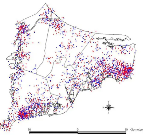
years prior to diagnosis. These data are described fully, including methodology for selection of cases and con-trols, demographics, and other features of the study pop-ulation, in the final report of the full study as well as follow-up papers on the breast cancer data; see [7,8] for further details. For illustration, the spatial distributions of breast cancer cases and controls (with no latency assump-tion) are shown in Figure 1.
Methods
The three statistical methods described here are: Bonetti and Pagano's M-statistic, based on the interpoint distance distribution [5]; Webster's GAM approach, which uses smoothing techniques [9]; and Kulldorff's spatial scan sta-tistic [10]. The M-statistic is a global unfocused test, mean-ing it is only concerned with departures of the spatial distribution of cases from the distribution of controls, without determining the location of any (possibly multi-ple) clusters or other differences. The GAM method maps disease odds ratios, provides a global test for deviation from a flat map, and identifies locations with significantly increased or decreased risk (here GAM is the conventional designation for Generalized Additive Model, not the Geo-graphic Analysis Machine of Openshaw [11], also used in cluster investigations). It incorporates a smoothing func-tion for locafunc-tion into a convenfunc-tional logistic regression
which accounts for effects of covariates. Kulldorff's scan statistic, the most widely used method for cluster investi-gations, scans the entire study region for local excesses and/or reductions of risk. Current implementations of the binary (Bernoulli model) version of the scan statistic allow adjustment for categorical covariates only, and the
M-statistic as implemented does not adjust for covariates at all (although allowing for categorical covariates via stratification would seem to be a straightforward exten-sion of the existing method). For simplicity we have cho-sen to apply all three methods to crude data only, thus avoiding the need to consider the differences in covariate adjustment across the three methods.
M-statistic
Bonetti-Pagano's M-statistic [5] is a non-parametric gen-eral test for clustering. It operates by representing and comparing the spatial distributions of two populations (here cases and controls) via the interpoint distance distri-bution. From any collection of n locations, we can calcu-late the roughly n2/2 interpoint distances between
locations and consider the distribution of these distances. Typically, a resampling procedure on the entire study pop-ulation is used to generate a baseline (or null) distribu-tion. Both the null distribution (estimated via resampling) and the observed distribution (calculated from the interpoint distances between cases) are binned into histograms, each of which can be represented as a vector. The test statistic is then a Malhalanobis-like dis-tance between the two vectors, weighted by an estimate of the covariance between histogram bins.
More formally, repeated resampling from the entire study population (cases and controls) is used to estimate the distribution of distances under the null hypothesis that both populations are sampled from the same spatial dis-tribution. Binning these distances and taking the mean over all iterations gives expected counts for each bin of the histogram. Experience with this method suggests that the optimal number of bins grows roughly on the order of where n is the number of cases being assessed (see also [12]). Denote by e the vector of expected values in each bin, expressed as a proportion of the total number of distances. Repeated resampling also allows us to estimate the covariance of e, which we will denote by S, a k × k
square matrix.
The interpoint distances for the disease cases are calcu-lated, binned, and written as a k-dimensional vector o, the observed bin values (expressed as proportions). Then the
M-statistic is:
M = (o - e)'S-(o - e)
Breast cancer cases and controls
Figure 1
Breast cancer cases and controls. Distribution of breast cancer cases (in red) and controls (in blue). Each point repre-sents the residence of one participant. Locations in this map have been geographically altered to preserve confidentiality. Actual residences were used in the analysis.
where S- is the Moore-Penrose generalized inverse of the
sample covariance matrix S. Thus we calculate the differ-ence between the expected (under the null hypothesis of no clustering) bin proportions and the observed bin pro-portions of the disease cases, inversely weighted by the covariance estimator. As S- is a positive semi-definite
matrix, M ≥ 0.
The asymptotic distribution of M is found in [5]. In prac-tice we can use the resampling procedure to calculate the distribution of M empirically under the null hypothesis. Comparing the calculated value of the test statistic to the null distribution gives a p-value that can be interpreted as the probability that the spatial distribution of the disease cases differs from the entire study population by chance alone.
GAM smoothing
Webster et al. [9,13] have used a procedure based on smoothing and generalized additive models (GAMs) to map disease and detect clusters (see [14] for related work). The generalized additive model predicts the log odds of disease (logarithm of the ratio of cases to controls) as a linear function of some covariates and a smooth function of spatial coordinates.
Specifically, the model specifies that for an individual with covariates zi and spatial location (xi, yi), the probabil-ity pi of disease is given by:
logit(pi) = S(xi, yi) + βzi
where βdenotes the vector of linear regression coefficients for the covariates. S(x, y) is a bivariate smooth function. Webster et al. use a loess (locally-weighted regression smoother) because it is adaptive to changes in data den-sity typically found in population maps. Around each point in the study area, a variable sized window is con-structed based on a predetermined number of nearest neighbors; within this window, the data contribute to S(x,
y) according to a tricube weighting function. Details are covered thoroughly in [15]. The window size (span) will affect both the bias and the variance (i.e. the amount of smoothing). Reducing the span reduces the bias but also increases the variance (reducing smoothness). Various cri-teria have been developed to balance these two properties of the smoother. Webster et al. use the Akaike Information Criterion (AIC), which averages the deviance but penal-izes the number of degrees of freedom. Minimizing the AIC estimates an "optimal" balance of bias and variance [15] in a computationally feasible manner. The global sta-tistic tests the null hypothesis of a flat map using the devi-ance of the model with and without the smoothing term. Among the available global test statistics, here we have used the deviance statistic [9]. The distribution of the
sta-tistic is estimated using permutation testing, with the case-control status permuted repeatedly. A pointwise test is then used to locate areas with significantly increased or decreased log odds relative to the map as a whole (the overall case-control ratio for crude analyses). The permu-tations also generate a distribution of the log odds at each location under the null hypothesis. The local p-value is determined by comparing the observed log odds with the null distribution.
After all statistical tests are performed, the log odds are converted to odds ratios using the entire study population as a reference. The odds ratios are mapped and significant "hot" and "cold" spots are delineated by drawing the .025 and .975 quantiles of the pointwise p-value surface. This graphical display is a natural part of the statistic and offers a rapid interpretation of the results of the calculations. The entire procedure can be run with existing software, e.g. S-Plus for the GAM and ArcView for mapping.
We note that care should be taken when interpreting the map of local p-values, because there is no adjustment for multiple testing. Thus under the null hypothesis of iden-tical spatial distributions of cases and controls, we can expect in general that statistically significant local p-values will occur at a higher rate than the Type I error rate speci-fied by the nominal alpha level. In other words, the local p-values are not to be used for hypothesis testing since we do not have adequate control of the Type I error rate. The local p-values do provide information about the measure of effect (in this case the local odds ratio), but inference based on these local p-values alone should be avoided.
Scan statistic
Kulldorff's scan statistic [10] has become the most widely used test for clustering in recent years, both because of its efficacy in detecting single hot (or cold) spots as well as the availability of the free software package SaTScan [16] for implementing the test. The basic idea of the scan sta-tistic is to allow circular windows of various sizes to range across the study region. At each location, the rate of dis-ease inside the window is compared to that outside the window. A hot (respectively cold) spot is characterized by a higher (lower) localized rate of disease.
Let denote the zone for which LZ achieves its
maxi-mum. This is called the most likely cluster, and we can cal-culate a test statistic via a likelihood ratio test. Let L0 = supp
= q L(Z, pZ, qZ) be the likelihood under the null hypothesis
(no clustering) and use
as the statistic of interest. The most likely cold spot is cal-culated similarly.
As with the other methods, inference is based on permu-tation of the case-control status. Under repeated permuta-tions, the distribution of λunder the null hypothesis is generated, and we compare the observed value of λto this distribution to yield a p-value. As noted above, SaTScan provides a relative risk for the most likely hot/cold spot, here an odds ratio inside the circle divided by an odds ratio outside the circle (hence not exactly comparable to the odds ratio computed by the GAM method).
For this study, we used the most recent version of the pub-licly available software [16] for analyzing binary (case-control) data, searching for either hot or cold spots.
Results
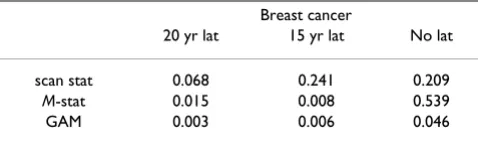
The three statistics in question were calculated for the breast cancer data with each of three latency periods. The results, showing global p-values for the M-statistic and the GAM method, and local p-value (for the identified "most likely cluster") for the scan statistic, are summarized in Table 1.
The three methods in general are not concordant when considered in a hypothesis testing context. However, all three methods are at least suggestive of significantly differ-ent spatial patterns for cases and controls when applied to the 20 year latency data set. The scan statistic result, while not significant at the customary 0.05 level, is nonetheless indicative of an excess of cases in the calculated most likely cluster, and contributes evidence towards a differ-ence between cases and controls when considered in the context of the results of the other two statistics. The smoothed map using the GAM method (Figure 2) shows one hot and one cold spot, a situation in which all three statistics are expected to maintain some reasonable sensi-tivity. The corresponding "most likely cluster" produced by the scan statistic is also shown (Figure 3). When applied to the breast cancer data set with 15 year latency,
both the M-statistic and the GAM indicate differences in the spatial distribution of cases and controls that are very unlikely to be explained by chance. The scan statistic, however, suggests that considered locally, random varia-tion remains a plausible explanavaria-tion. Examinavaria-tion of the smoothed map (Figure 4) shows two distinct and promi-nent hot spots in the data, and one cold spot. The pres-ence of multiple clusters in the data may partially explain the divergent results. The associated scan statistic output is also shown (Figure 5).
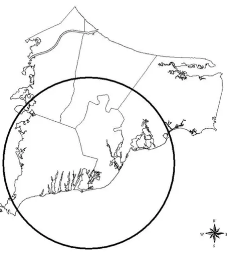
When no latency is considered for breast cancer, the M -statistic is no longer -statistically significant, making the GAM the only method that offers strong evidence against chance alone explaining the spatial patterns in the data. Figures 6 and 7 show the smoothed map for this data set as produced by the GAM and the cluster identified by the scan statistic, respectively. The GAM map shows a broad, diffuse area of increased risk (odds ratios (ORs) roughly 2.0) along the coast and periphery in the northern Cape Cod area. Kulldorff's likelihood-based method identifies the same area and roughly the same relative risk (RR), but the local excess of cases is not statistically significant. Both methods are detecting a single hot spot, but it is elongated instead of the optimal (circular) configuration for Kull-dorff's method. The M-statistic provides no evidence of global differences at the significance level of 0.05, perhaps due to the diffuse nature of the apparent hot spot. Thus the evidence for clustering in this data set is mixed.
Discussion
The discussion of results presented here should not be construed as epidemiologic findings, but rather the out-put of three statistical methods as applied to real data. The maps produced are for illustration purposes only, and should not be interpreted epidemiologically (one reason being that we have not controlled for covariates).
We remark that the common use of the word "cluster" to describe a disease hot spot represents only one kind of departure of spatial difference between cases and controls. The scan statistic alone restricts itself to this particular
LZ L Z p q
p q
Z Z
=
>
sup ( , , )
ˆ
Z
λ = L L
Zˆ
0
Table 1: p-values associated with cluster statistics. Results (p-values) of analysis using the scan statistic, the M-statistic, and the GAM method with deviance statistic.
Breast cancer
20 yr lat 15 yr lat No lat
kind of spatial difference and further places emphasis on the single most likely circular hot or cold spot. We have chosen to adopt here the broader but more flexible objec-tive of detecting any difference in the spatial distribution of cases compared to the controls. The problem of locat-ing and quantifylocat-ing local excesses or deficits is clearly important, and both the scan statistic and the GAM address this problem directly. The M-statistic does not, although extensions of distance-based methods to the problem of cluster location are currently being developed [17].
We have presented applications of three well-developed and theoretically-grounded methods to detect spatial dif-ferences in the distribution of cases and controls in a real data set. The different patterns seen in this data set, com-prising breast cancer with different latency considerations, affect the outcomes of these methods. We have identified at least three features that plausibly are involved (the shape, number, and intensity of areas of inhomogeneity), but there are likely others present here and in other real data sets. For example, methods may have different sensi-tivity depending on the areal size and/or location of spatial differences. In these cases, the sensitivity of each
method may differ depending on location of a particular hot or cold spot, even when size, shape and intensity of the hot/cold spot are comparable (e.g. differing "edge effects" across methods).
Each of these methods would be expected to have certain strengths and weaknesses. The M-statistic has been imple-mented both in case-control studies [5], and in surveil-lance settings [18] where there is a large amount of historical data to use as a baseline for the null distribution of distances. Simulations suggest that it has the potential to be sensitive to situations such as multiple hot spots, where other statistics (such as the scan statistic) may lose power [3,4], but these same studies show that the M -sta-tistic will typically underperform other sta-sta-tistics when there is a single hot spot to detect.
Provided there is some historical record, or sufficiently large control population from which to resample, the M -statistic can handle small sample sizes adequately. This is important in a surveillance setting, and is an advantage over rate-based statistics that may have insufficient data in the small sample case to draw proper inferences. In envi-ronmental settings these situations may arise in small, neighborhood-sized population studies.
Breast cancer 20 year latency (GAM)
Figure 2
Breast cancer 20 year latency (GAM). Breast cancer 20 year latency, GAM smoothed rate map. Solid lines delineate areas where the point-wise GAM deviance statistic is less than 0.05.
Breast cancer 20 year latency (scan)
Figure 3
However, as currently implemented the M-statistic does not adjust for covariates, but instead is used on raw spatial data only. The origins of the M-statistic lie in public health surveillance where spatial confounders are implicitly accounted for in the immediate historical record. As noted above, the M-statistic does not locate hot spots, but rather detects a difference between the two populations under comparison. Because these differences are quantified via the interpoint distance distribution and not the geo-graphic locations of cases and controls themselves, results do not have a direct interpretation as do the "most likely cluster" of the scan statistic or the local odds ratios of the GAM.
GAM smoothing is a robust data-based approach that can be run with standard software. The ability to map disease outcomes while adjusting for covariates in a way familiar to epidemiologists is a particular strength. It is semi-para-metric, assuming a linear model in the covariates with an additive spatial effect. Ignoring covariates and considering the data on a purely spatial basis there are essentially no statistical assumptions required, although the choice of window size may affect the sensitivity of the smoothing approach. The GAM approach provides global statistics to test the map for overall deviation from flatness as well as a pointwise test to locate areas of significantly elevated
and decreased disease risk. Sufficient sample size for sta-ble rates is also important, and results for small sample sizes are difficult to interpret meaningfully.
The scan statistic will certainly excel [3,4] when there is a single hot spot present and that hot spot is roughly circu-lar in shape. The model assumption of a Bernoulli distri-bution inside and outside a circular region can be suboptimal if either the hot/cold spot is not circular, or if there is more than one spot present. There has been additional work on the scan statistic focusing on examin-ing or improvexamin-ing robustness to the shape of the hotspot [19-21].
The scan statistic is especially appealing because of its immediate identification of the most likely cluster. Public availability of the implementation via the SaTScan soft-ware has increased its popularity and visibility. Perhaps most importantly, the method's exceptional power to detect single hot spots deserves consideration in situa-tions where a single hot spot scenario seems plausible, or even possible. As a rate-based approach, the scan statistic is also limited to sample sizes that provide stable rate estimates.
Aggregated data can be handled using a Poisson model, similar in spirit to the Bernoulli model used for case-con-trol data. The currently available software can adjust for covariates in the Poisson case, and adjustments for
Breast cancer 15 year latency (GAM)
Figure 4
Breast cancer 15 year latency (GAM). Breast cancer 15 year latency.
Breast cancer 15 year latency (scan)
Figure 5
categorical variables in the Bernoulli model are allowed in the most recent release of the SaTScan software.
Multiple hot/cold spots would seem to be problematic when using the scan statistic, since it uses a likelihood function from a model based on a single hot or cold spot only. Placing restrictions on the underlying probability model clearly results in higher power when the model is correctly specified, but the presence of multiple clusters would imply that the scan statistic has misspecified the model. Thus we should expect that in some of these situations the scan statistic may suffer loss of power. The GAM and M-statistic would be expected to be sensitive to a wider variety of multiple cluster arrangements, but this flexibility is inherent in the global nature of these test sta-tistics in contrast to the essentially local nature of the scan statistic.
The published results cited above indicate that for the benchmark simulated data considered, the scan statistic is quite robust to some multiple cluster arrangements. We note that these comparisons are dependent on the simu-lated data used for the purposes of the power study. Mul-tiple hot/cold spots may be common occurrences in real data sets, and a more thorough effort to generate realistic
simulations for these data is a direction for future research.
Likewise, there is no reason to assume that areas of increased risk will be any particular shape, especially as neither underlying population nor possible exposures are similarly constrained. Several recent papers have contin-ued investigation of the scan statistic and its performance when dealing with non-circular hot spots (as well as extensions of the methodology to improve robustness in these situations); see for example [17]. As with the issue of multiple hot spots, more work may be needed to simulate such data in a realistic manner. We again emphasize the importance of studies that consider real data in addition to synthetic data, and the potential to learn from both types of data as spatial methods continue to develop and improve.
Conclusion
With the variety of approaches to the problem of examin-ing spatial patterns of disease, it is not surprisexamin-ing that some methods are more effective than others for detecting certain patterns. A better understanding of the relative strengths and weaknesses of the various methods is essen-tial to appropriate choices of methodology. Studies of spatial distribution of disease will also benefit from the information available from a variety of statistical
Breast cancer no latency (GAM)
Figure 6
Breast cancer no latency (GAM). Breast cancer no latency.
Breast cancer no latency (scan)
Figure 7
Publish with BioMed Central and every scientist can read your work free of charge "BioMed Central will be the most significant development for disseminating the results of biomedical researc h in our lifetime."
Sir Paul Nurse, Cancer Research UK
Your research papers will be:
available free of charge to the entire biomedical community
peer reviewed and published immediately upon acceptance
cited in PubMed and archived on PubMed Central
yours — you keep the copyright
Submit your manuscript here:
http://www.biomedcentral.com/info/publishing_adv.asp
BioMedcentral
methods, and careful consideration of the complemen-tary nature of this information should assist in the inter-pretation of results of studies with a spatial component.
To this point, much of the work in gaining this under-standing has come from analyzing synthetic data, where the underlying model can be controlled and various fea-tures superimposed in order to perform a careful study of these strengths and weaknesses. However, some character-istics of real data sets may be hard to simulate with syn-thetic data, or may not be readily apparent in advance of analysis and further study, and results based on simulated data are at least partially dependent on the particular sim-ulations themselves.
The comparative analyses by different methods of real data sets point to directions for further research of the properties of each of the statistics used in this paper. We suggest a further research program designed around alter-nately examining real and simulated data sets for these kinds of differences, in order to develop the practical application of statistical methods to epidemiological data with a spatial component.
List of abbreviations
AIC: Akaike Information Criterion
GAM: Generalized Additive Model
GIS: Geographic Information System
OR: Odds Ratio
RR: Relative Risk
Competing interests
The author(s) declare that they have no competing interests.
Authors' contributions
AO and VV were responsible for statistical programming. All authors contributed to writing and editing.
Acknowledgements
AO's research partially supported by NIH grant RO1-AI28076 and NLM grant RO1-LM007677. TW, VV, DO, JW, and AA are supported by Super-fund Basic Research Program 5P42ES 07381.
References
1. Lawson A, Biggeri A, Böhning D, Lesaffre E, Viel JF, Bertollini R: Dis-ease Mapping and Risk Assessment for Public Health Wiley; 1999. 2. Forsberg L: A review of clustering literature for public health.
. [Preprint]
3. Kulldorff M, Tango T, Park PJ: Power comparisons for disease clustering tests. Comp Stat Data Anal 2003, 42:665-684. 4. Ozonoff A, Bonetti M, Forsberg L, Pagano M: Power comparisons
for an improved disease clustering test. Comp Stat Data Anal 2005, 48:679-684.
5. Bonetti M, Pagano M: The interpoint distance distribution as a descriptor of point patterns: An application to cluster detection. Stat Med in press.
6. Aschengrau A, Ozonoff D: Upper Cape Cancer Incidence Study, Final Report. .
7. Aschengrau A, Paulu C, Ozonoff D: Tetrachloroethylene-con-taminated drinking water and the risk of breast cancer. Envi-ronmental Health Perspectives 1998, 106:947-953.
8. Aschengrau A, Rogers S, Ozonoff D: Perchloroethylene-contam-inated drinking water and the risk of breast cancer: Addi-tional results from Cape Cod, Massachusetts, USA. Environ Health Perspect 2003, 111:167-173.
9. Webster T, Vieira V, Weinberg J, Aschengrau A: Spatial analysis of case-control data using generalized additive models. In Pro-ceedings from EUROHEIS/SAHSU Conference: 30–31 March 2003; Öster-sund, Sweden Edited by: London JL. Small Area Health Statistics Unit; 2003:56-69.
10. Kulldorff M: A spatial scan statistic. Commun Statist Theory and Methods 1997, 26:1481-1496.
11. Openshaw S, Charlton M, Wymer C, Craft A: A mark i geograph-ical analysis machine for the automated analysis of point data sets. Intl J Geographic Information Systems 1987, 1:335-358. 12. Mann HB, Wald A: On the choice of the number and width of
classes for the chi-square test of goodness of fit. Annals of Math Stat 1942, 13:306-317.
13. Webster T, Vieira V, Weinberg J: A method for mapping popula-tion-based case-control studies using generalized additive models. . [Preprint]
14. Kelsall J, Diggle P: Spatial variation in risk of disease: A nonpar-ametric binary regression approach. Journal of the Royal Statisti-cal Society, Series C 1998, 47:559-573.
15. Hastie TJ, Tibshirani RJ: Generalized Additive Models Chapman and Hall; 1990.
16. SaTScan v 5.0 [http://www.satscan.org]
17. Ozonoff A, Bonetti M, Forsberg L, Pagano M: The distribution of distances, cluster detection, and syndromic surveillance.
2004 Proceedings of the American Statistical Association, Biometrics Section 2004.
18. Ozonoff A, Forsberg L, Bonetti M, Pagano M: A bivariate method for spatio-temporal syndromic surveillance. MMWR 2004,
53S:61-66.
19. Kulldorff M, Nagarwalla N: Spatial disease clusters: detection and inference. Stat Med 1995, 14:799-810.
20. Kulldorff M, Zhang Z, Hartman J, Heffernan R, Huang L, Mostashari F:
Benchmark data and power calculations for evaluating dis-ease outbreak detection methods. MMWR 2004, 53S:144-151. 21. Tango T, Takahashi K: A flexibly shaped spatial scan statistic for