Relay Feedback Based Time Domain Modeling of Linear
3-by-3 MIMO System
Sujatha V, Rames C. Panda
*Department of Chemical Engineering, CLRI (CSIR), Adyar, Chennai, 600020, India
Abstract
Relay feedback tests are carried out on multi input multi output systems. Analytical expressions for relay responses in time domain for the interactive transfer functions (off-diagonal elements) of the systems are derived and are validated. Generalized expressions are formulated based on the observation that a relay feedback test consists of a series of step inputs and a stable limit cycle implies a convergent infinite series. MIMO systems with lower-order transfer functions with different time delays are used to illustrate the derivation. These analytical expressions, in a closed form solution areuseful to identify unknown system parameters, to understand interactions, to diagnosis the fault at the earlier stage, and
subsequently for auto tuning. This closed-loop equation not only enables us to assess the effect of interactions between in-puts and outin-puts but is also useful to back calculate/estimate the exact process model parameters, appearing in the analyti-cal expressions for linear 3-by-3 MIMO systems, from experimental response.
Keywords
Modelling, Relay Feedback, Identification, Auto Tuning, Multi Input Multi Output1. Introduction
Chemical processes are complex and non-linear in nature due to interactions (Seborg et. al, 2004) between inputs and outputs. With increase in complexity of the process, it be-comes difficult to control the loops properly. Whenever closed loop performance degrades, loops must be retuned with correct input-output pairs. The sequential identification and the expert controller design methods form the basic structure for the multivariable autotuner that allows loop tuning without breaking the loop and without interrupting production, in process industries.
The relay feedback test was first proposed by Astrom and Hagglund (1984) for process control practitioners as a closed-loop tool for system identification and control. In this method (Astrom and Hagglund, 1984), periodic step func-tions are given as input to the unknown process and outputs
are collected (that lags behind input by π radians) from
which limit cycle data (Ku and Wu) are found to approxi-mate the process model parameters. Many researchers (Luyben, 1987; Yu, 1999; Majhi and Atherton, 1999; Wang et.al., 1997) have worked on autotuning of PID controller for low order systems and have reported of getting more infor-mation and better performance of closed-loop system. Re-ports have also been presented on formulating mathematical models (Thyagarajan & Yu, 2002; Panda & Yu, 2003; Lee &
* Corresponding author: Email. Published online at http://journal.sapub.org/ajss
Copyright © 2012 Scientific & Academic Publishing. All Rights Reserved
This paper is organized as follows: introduction to relay feedback test on MIMO process was detailed in section 2 followed by general description of typical 3x3 multivariable processes. In section 4, modeling equations for relay re-sponses of 3x3 processes are developed. Analytical expres-sions thus obtained, are validated in section 5 for relay feedback responses through modeling in order to character-ize the undesired responses. The simulation results on some 3x3 processes are characterized in section 6. Concluding remarks are drawn in the final section.
2. Relay Feedback Test on MIMO
Process
Based on the concept of sequential auto tuning (Shen & Yu,[8]) method each controller is designed in sequence. Let’s consider a 3-by-3 MIMO system with a known pairing
(y u1− 1), (y2−u2) and (y u3− 3) under decentralized PI
con-trol (Figure 1). Initially, an ideal relay is placed between y1
andu1, while loop 2 and loop 3 is on manual. Following the
relay-feedback test, a controller can be designed from the ultimate gain and ultimate frequency. The next step is to perform relay-feedback test between y2 and u2 while loop
1 is on automatic and loop 3 is on manual. Finally, re-lay-feedback test between y3 and u3 while loop 1 and loop
2 is on automatic, a controller can also be designed for loop 3 following the relay-feedback test. This procedure is repeated until the controller parameters converge. Typically, the controller parameters converge in 3 - 4 relay-feedback tests for 3-by-3 MIMO systems.
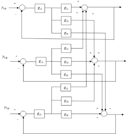
Figure 1. Closed loop representation of 3-by-3 MIMO process with decentralized control structure
The 3-by-3 MIMO process with decentralized control structure is shown in Figure. 2. For 3-by-3 MIMO system, described by Eq. (2.1) as
1 11 12 13 1 2 21 22 23 2 3 31 32 33 3
y g g g u
y g g g u
y g g g u
=
(2.1)
The decentralized controller is described by Eq. (2.2) as
( )
1 23
0 0
0 0
0 0
c
c c
c G
G s G
G
=
(2.2)
As it is evident from closed-loop sequential auto tuning, for a 3-by-3 system, we come across G11,CL , G22,CL and
33,CL
G as diagonalised transfer functions (that govern basic
transfer functions for controller design) and interactive transfer functions as G12,CL, G13,CL, G21,CL, G21,CL, G31,CL
and G32,CL.
The effective closed loop relation between y2 and u1 for 3-by-3 MIMO system is
(
23 31)
2121,
2 22 3 33 3 33
1 1
CL
c c c
g g g
G
G g G g G g
= −
+ + (2.3)
21 21 21
21 1 D s k e g
s
τ
−
=
+ ;
22 22 22
22 1 D s k e g
s
τ
−
=
+ ;
23 23 23
23 1 D s k e g
s
τ
−
=
+ ;
31 31 31
31 1 D s k e g
s
τ
−
=
+ ;
33 33 33
33 1 D s k e g
s
τ
−
=
+ ;
2 2
2
1 1
c c
i
G k
s
τ
= +
Figure 2. Block diagram of nxn multivariable systems with decentralized PI controller
3. Description of 2x2 System and 3x3
System
Let us consider squared MIMO systems of 2 x 2 and 3x3 types:
The interactive transfer functions for 2 x 2 and 3 x 3 sys-tem are gp12 and gp21. The effective closed loop relation
between y2 and u1 for 2x2 system is
21 21,
2 22 1
p p cl
c p
g g
G g
=
+ where,
21 21 21
21 1 D s
p k e
g
s
τ
−
= +
22 22 22
22 1 D s
p k e
g
s
τ
−
=
+ and
2 2
2
1 1
c c
i
G k
s
τ
= +
2x2 system 3x3 system
( ) 11 12 21 22
p p
p
p p
g g
g s
g g
=
( ) 1 2
0 0c c
c
G G s
G
=
( ) [1( ) 2( )]T
u s = u s u s
( ) [ 1( ) 2( )]T
y s = y s y s
( ) 1121 1222 1323 31 32 33
p p p
p p p p
p p p
g g g
g s g g g
g g g
=
( ) 1 2
3
0 0
0 0
0 0
c
c c
c
G
G s G
G
=
( )
[
1( ) 2( ) 3( )]
T u s = u s u s u s( )
[
1( ) 2( ) ( )3]
T y s = y s y s y s21 21,
2 22 1
p p cl
c p
g g
G g
=
+
(
)
21 23 31 21,
2 22 3 33 3 33
1 1
p p p p cl
c p c p c p
g g g
g
G g G g G g
= −
+ +
The effective closed loop relation between y2 and u1 for
3x3 system is
(
)
21 23 31
21,
2 22 3 33 3 33
1 1
p p p
p cl
c p c p c p
g g g
g
G g G g G g
= −
+ +
31 23
31 23
31 23
31 1 23 1
D s D s
p k e p k e
g g
s s
τ τ
− −
= =
+ + 2 2 2
1 1
c c
i
G k
s
τ
= +
(3.2)
4. Modeling of 2x2 and 3x3 System
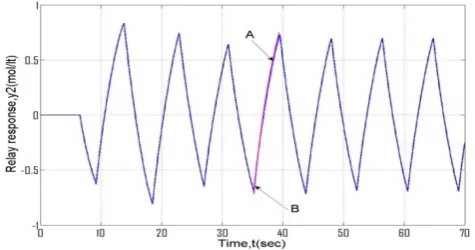
Figure 3a. Relay feedback response of 3x3 systems (OR distillation column)
Figure 3b
.
Validation of analytical expression of 3x3 interactive cross TF with experimental relay response (OR column)Mathematical models are developed to represent relay responses produced by closed loop interaction transfer function for 3 input 3 output systems (Eqn. 3.2). It is as-sumed that relay output is generated by a series of small number of step changes in manipulated variable. Hence the
stabilized output is a sum of infinite terms of small responses due to those step changes. The typical relay feedback re-sponse of closed loop interaction transfer function of 3x3 systems is shown in Figure 3a.
4.1. The Relay Response of 3x3 MIMO Systems
For 3x3 systems the relay responses obtained from inter-active transfer functions are modeled as follows. The relay response is assumed to be formed by n-number of small step changes. At the first interval, the response can be described as
( )
( )
22 2
21 22
1 21 2 22
2
23 31 3 3 23 33 33 3 33
1 2 3 3 33
3 33 3
1 1
1 1
t t
c i i
t t t t
i i c
i
c i
k k
y k e e
k k a e a e a e k k e
k k
τ τ
τ τ τ τ
τ τ τ
τ τ τ
τ
− −
− − − −
= − − + − −
− − + + − + −
(4.1)
Where
(
)
(
3)(
3 33)
(
23(
23)(
33)
)
(
31(
31)(
33)
)
1 2 3
3 23 3 31 23 3 23 31 31 3 31 23
; ;
i i
i i i i
a = τ ττ τ τ−τ τ a = ττ ττ τ−τ τ a = ττ ττ τ−τ τ
− − − − − −
Let D D= 23+D31−D33, at the second instant, the relay
output can be given by
(
)
(
)
21
21 21
2 21
22
22 2 22 22
2 22 2 22
2
3 23 31
1 2 3
23 31 3 3 33
3 23
1 2
1 2 1
1 2 1
1
2
t D t
t D t
c
i i
i
t D t D t D
i i
t t
c
i
y k e e
k k e e
a e a e a e k k
k k
a e a e
τ τ
τ τ
τ τ τ
τ τ
τ τ τ τ
τ
τ
+
− −
+
− −
+ + +
− − −
− −
= − − − −
+ − − + − −
− + + −
+ −
(
)
(
)
31 3
33
33 3 33 33
3 33 3 33
3
1 2 1
t
t D t
c
i i
i
a e
k k e e
τ
τ τ
τ τ τ τ
τ
−
+
− −
−
+
+ − − + −
(4.2)
The above equation (4.2) can be simplified as
[ ]
[ ] (
)
21
21 21
2 21
22
22 2 22 22
2 22
2
3 3 23 23
1 2
23 31 3 3 33
31 31
1
1 2 2
1 2 2
2 2
1
2
D t
D t c
i i
t D t D
i i
i
t D
c
y k e e
k k e e
a e e a e e
k k k k
a e e
τ τ
τ τ
τ τ τ τ
τ τ
τ τ τ
τ
− −
− −
− − − −
− −
= − − −
− − + − − −
− + −
−
+ −
−
[ ] (
)
3333 3 3 33 33 33
3
1 2 2
D t c
i i
k k τ τ eτ eτ
τ
− −
−
− − + − −
At the third instant,
21 2 21
21 21 21
3 21 1 2 1 2 1
pu
t D t D t
y k e τ e τ e τ
+ + + − − − = − − − + − − ( ) ( ) ( )
22 2 22
22 22
2 22 2 22
22 2 2 22 2 22 2 2 3 23
1 2 3
23 31 3 3 33
1 2 1
2 1
1
pu
t D t D
i i
c
i t
i
pu pu
t D t D t D
i i c e e k k e
a e a e a e
k k k k τ τ τ τ τ τ τ τ τ τ τ τ τ + + + − − − + + + + + + − − − + − − + − − − + + − + + − − 2 31
3 23 31
1 2 3
3 23 31
1 2 3
2
2
pu
t D t D t D
i
t t t
i
a e a e a e
a e a e a e
τ τ τ τ τ τ τ + + + − − − − − − − − + + − + + + ( ) ( ) ( ) 33 33 2 33 33
3 33 3 33
33 3 3
33 3 33
1 2 1
2 1
pu
t D t D
i i c i t i e e k k e τ τ τ τ τ τ τ τ τ τ + + + − − − + − − + − + + − (4.3)
This eq. (4.3) can be simplified as
[ ]
[ ] ( )
21 2 21 21 21 21 3 21
22 2 22
22 2 22 22 22
2 22 2
2 3 3 1
23 31 3 3 33
1 2 2* 2
1 2 2* 2
2* 1 pu D D t pu D D t c i i pu D t D i i i c
y k e e e
k k e e e
a e e e
k k k k τ τ τ τ τ τ τ τ τ τ τ τ + − − − + − − − + − − − = − − − + − − + − − + − − − − 3 2
23 23 23 2
2
31 31 31 1 2 2* 2 2* 2 i pu D t D pu D t D
a e e e
a e e e
τ τ τ τ τ τ τ + − − − + − − − − + − − + − − [ ] ( )
33 2 33
33 3 3 33 33 33 33
3
1 2 2* 2
pu D D t c i i
k k τ τ eτ e τ e τ
τ + − − − − − − + − − −
As time tends to infinity, the response becomes stabilized. Thus, the overall response can be described as
[
]
1 1
21 2 2
1 1 2
21 21 21 21
21 1 2 2 ... 2 ... 2 2
n p n p
u u p
D u
t n n
t
y k eτ e τ e τ e τ
− − − + = = − − − − ∑ ∑ = − + − − − + + − − [ ] ( ) 1 1
22 2 2
1 1 2
22 2
22 22 22 22
2 2 22
1 2 2 ...
2 ...2 2
n pu n pu
p
D u
t n n
c
i i
k k
eτ e τ e τ eτ
τ τ τ − − − + = = − − − − + − ∑ ∑ − + − − + − −
1 1 1
2 2 2
1 1 1
3 3 3 3
1
1 1 1
2 2 2
1 1 1
23 31 3 23 23 23 23
2 3 33
31 1
2* 2... 2* 2
1 2* 2... 2* 2
n pu n pu n pu
D
t n n n
i i i i
n pu n pu n pu
D
t n n n
i c
D t
a e e e e
k k a e e e e
k k
a e e
τ τ τ τ τ τ τ τ τ τ − − − + − − − − − − − + − − − − − − = = = = = = ∑ ∑ ∑ − + + − + ∑ ∑ ∑ − + − + + − +
− 1 1 1
2 2 2
1 1 1
31 2* 31 2... 2* 31 2
n pu n pu n pu
n n n
e e τ τ τ − − − + − − = = = ∑ ∑ ∑ − + + + −
[ ]
(
)
1 1 1
33 2 2 2
1 1 1
33 3
33 33 33 33
3 3 33
1 2
2* 2... 2* 2
n pu n pu n pu
D
t n n n
c
i i
k k
eτ e τ e τ e τ
τ τ τ − − − + − − = −= −= − − ∑ ∑ ∑ − + − − + + − (4.4)
The above eq (4.4) can be written as
{
}
{
}
(
)
{
}
21 22 2 2 23 31 33 33 33 3
3
sec
1 s
{ nt }
t c i i c c i
y k firstpart ondpart k k thirdpart fourthpart
k k fifthpart ixthpart seventhpart k k
k k eigthpart ni hpart τ τ τ = − − + − − − + + − +
Let 2 21
1
pu
r eτ
−
= ; 2 22 2
pu
r eτ
−
= ; 2 3
3
pu i
r eτ
−
= ; 2 23 4
pu
r eτ
−
= and 2 33
5
pu
r eτ
−
=
The RHS of the above series becomes First part = [1-2+2-2+…..] = 1 In similar way, third part = 1
21
1 2 21
1 1 1 1
Secondpart 2 2 2 .... 2 2
D
n n n
e−τ r r − r − r
= − + − + − This second
part can be put into following series
2 3
1 1 1
1
2 21
2 2
2 1 ...
1
1 pu
thirdpart r r r
r
e− τ
= − + − + = =
+ +
In similar way,
2 2 22
2 2 fourthpart= 1 1 pu r e−τ
= +
+
3 2 3
2 2 fifthpart= 1 1 pu i r
e− τ
= + + ; 4 2 23 2 2 sixthpart= 1 1 pu r
e− τ
= +
+
5
2 33
2 2
seventhpart= 1
1
pu r
e− τ
= +
+
The generalized analytical expressions for 3x3 system is given by
( )
22 2
21 22
21 2 22
2
221 221
3 23 33
1 2 3
2 3 223 233
2 2
1 1
1 1
2 2 2
1
1 1 1
t t
c
n pu i i pu
t t t
i
pu pu pu
i
k k
y k e e
e e
a e a e a e
e e e
τ τ
τ τ
τ τ τ
τ τ τ
τ τ τ
− −
− −
− − −
− − −
= − − + −
+ +
− + +
+ + +
−
( )
33 3 33
3 33
3 2 33
2 1
1
t c
i pu
i
k k e
e
τ τ
τ τ τ
−
−
−
+ −
+
(4.5)
after normalizing 23 31 3
3 33
i c
k k k k
τ to unity and assuming
( 22) 1
y t D− = ; y t D( − 33)=1, eq. (4.5) can be simulated and
Figure 3b and Figure 4a can be generated.
5. Validation of Analytical Expressions
for 2x2 and 3x3 Systems
The transfer function of Ogunike & Ray (OR) distillation column is given by
2.6 3.5
1 3 3 1.2
2
3 9.2 9.4
0.66 0.61 0.0049
6.7 1 8.64 1 9.06 1
2.36 2.3 0.01
5 1 5 1 7.09 1
34.68 46.2 0.87(11.61 1)
8.15 1 10.9 1 (3.89 1)(18.8 1)
s s s
s s s
s s s
e e e
s s s
y
e e e
y
s s s
y
e e s e
s s s s
− − −
− − −
− − −
− −
+ + +
− − −
=
+ + +
− +
+ + + +
1 2 3 u u u
(5.1)
The above transfer function represents multiproduct plant distillation column for the separation of binary mixture of ethanol-water (Ogunnaike-Ray (OR) column). The top compositions (y) are controlled by manipulating the reflux (V) and the reboiler steam flow rates and pressure. Feed flow rate (F) is disturbance. It can be noted that gp33(s) can be approximated to FOPDT model structure (Skogestad, 2003) after which relay response can be generated using simulink (experimental). Responses obtained after simulating OR column (in simulink) are compared with its original relay responses (obtained by simulating Eq. 4.5). Figure 3b and Figure 4a show the validation of derived mathematical models where theoretical response matches exactly with simulated (simulink platform) one. Figure 3b shows inter-active transfer function of OR colums. AB is response of theoretical equation while the other continuous curve is generated from experiment. Figure 4a presents validation of one-loop of interactive transfer function of 3x3 column OR system under measurement noise. Figure 4b shows the validation of undesired-relay feedback responses for
real-time liquid level system.
Figure 4a. Validation of analytical expression (AB) of 3x3 interactive cross TF with experimental relay response in the presence of measurement noise (OR column)
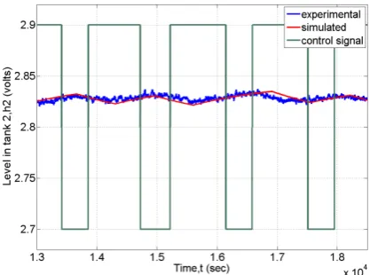
Figure 4b. Validation of analytical expression (smooth) of 2x2 interactive cross TF with real time experimental relay response(noisy) in the presence of measurement noise (Liq level system)
Experimental setup: The coupled tanks set-up is a model of a liquid storage system in process industries. Often tanks are coupled through connecting pipes. These storage facili-ties contain fluids where the reactant level and flow are to be controlled. Water is chosen as the fluid. The experiment set-up of coupled tanks is designed so that the system can be configured. The set-up has four translucent tanks each with a pressure sensor to measure the water levels. The couplings between the tanks can be modified by the use of seven manual valves to change the dynamics of the system im-posing the use of different controllers. Water is delivered to the tanks by two independently controlled, submersed pumps. Step disturbances on the flowrate are provided by four manual valves. Drain flow rates can be modified using ori-fice caps that are easy to change. The 33-041 coupled tank system is interfaced with computer through MATLAB / SIMULINK and an Advantech PCI 1711 data acquisition interface card.
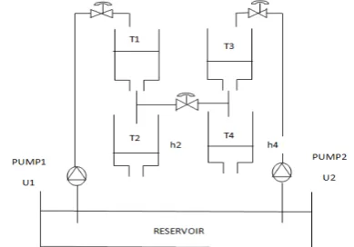
as shown in Figure 5 has been used to control the levels in the lower two tanks with two pumps. The process inputs are u1 and u2 (input voltages to excite the pumps) and the outputs are h4 and h2 (heights from level measurement devices). The design parameters of the coupled tanks experimental set up
are cross-sectional area of each tank, A=0.01389m2; outlet
(exit pipe) area of tank, a=50.2658x10⁻⁶ m2 and gravitational constant, g=9.81 m/s2. A step disturbance on u1 is given and changes in h4 and h2 are recorded. Similar step responses in levels for step disturbance on u2 are also collected. Figure 4b shows the validation of undesired-relay feedback responses for real-time liquid level system.
Figure 5a. Experimental setup for two interacting tank level control system
Figure 5b. Schematic diagram of coupled tanks experimental set up
6. Conclusions
A systematic approach is proposed to derive exact ex-pressions for relay feedback responses for diagonal and interactive transfer functions in MIMO systems. The closed loop interaction transfer functions of 3x3 systems were modeled without using approximation of time delay. These results are provided in a closed form solution for the first time. These model equations are useful to back calculate the exact process model parameters. Moreover, as these inter-active transfer functions carry information on interactions between inputs/outputs, these theoretical models will pro-vide information on measuring interactions directly. This breakthrough will also help in assessing interaction measures between inputs-outputs.
ACKNOWLEDGEMENTS
The authors are willing to acknowledge the financial aid of project (SR/S3/CE/090/2009) sponsored by DST in car-rying out this research work.
REFERENCES
[1] Astrom. K. J.; Haagglund, T., Automatic tuning of simple regulators with specifications on phase and amplitude mar-gins, Automatica,1984, 20, 645-651
[2] Seborg D E, T F.Edgar and D A. Mellichamp, Process Dy-namics and Control, 2nd edn. 2004, John Wiely and Sons, NJ.,
478-80
[3] Luyben, W. L., Getting more information from relay feed-back tests, Ind. Eng. Chem. Res. 2001, 40, 4391-4402. [4] Majhi, S N, On-line PI Control of stable processes, Journal of
Proc control, 15, 2005, 859-867.
[5] Majhi, S N, Relay- based identification of a class of Non minimum phase SISO Processes, IEEE Trans on Autom control, 52, 2007,134-139.
[6] Panda R C and C.C. Yu, Analytical expressions for relay feedback responses, Journal of. Proc. Control 13 (6), 2003, 489–501.
[7] Skogestad, S., Simple analytical rules for model reduction and PID controller tuning, Journal of Proc. Control, 13, 2003,
291-309
[8] Tao Liu and Furong Gao, A systematic approach for online identification of second order process model from relay feedback tests, AIChE Journal, 54 (6), 2008,1560-78. [9] Thyagarajan T and C.C. Yu, Improved auto-tuning us-ing
shape factor from relay feed back, Ind. Eng. Chem. Res. 42, 2003, 4425–4440.
[10] Vivek S. and Chidambaram M, An improved relay au-totuning of PID for unstable FOPDT systems, Comp and Chem Engg, 29, 2005, 2060-2068.
[11] Yu, C.C., Auto-Tuning of PID Controllers, 1999, Springler –Verlag, London.
[12] Panda, R. C. and Yu. C.C., Exact analytical expressions for relay feedback responses – second order plus dead time processes, Asian Cont Conf., Singapore, 2002, 25-27 Sept. [13] Wu Y., Luo H., Ming D., Zou J. and Li Xiuna, Efficient
limited feedback for MIMO relay systems, IEEE Communi-cations Letters, 2011, 15(2), 181-183.
[14] Lee J., Jin-su Kim, Byeon J., Sung Su W. and Edgar TF, 2011, 57(7), 1809-16