Modeling of Transition Processes in a Partially Invariant Center of Mass Motion Stabilization System

Modeling of Transition Processes in a Partially Invariant

Center of Mass Motion Stabilization System

Nickolay Zosimovych

Intelligent Manufacturing Key Laboratory of Ministry of Education, Shantou University, Shantou, China

Abstract The publication suggests how to significantly improve the spacecraft centre of mass movement stabilization

accuracy in the active phases of trajectory correction during interplanetary and transfer flights, which in some cases provides for high navigation accuracy, when rigid trajectory control method is used. The required stability conditions obtained are consistent with the known criteria in the invariant theory. Computer modelling shows that in a partially invariant stabilization system reveals the significant advantages of such a system in terms of greater accuracy when compared to known stabilization systems.

Keywords Space vehicle (SV), Stabilization controller (SC), On-board computer (OC), Gyro-stabilized platform (GSP),

propulsion system (PS), Angular velocity sensor (AVS), Operating device (OD), Feedback (FB), Control actuator (CA), Control system (CS), Angular stabilization (AS), Centre of mass (CM)

1. Introduction

The thriving space technology is characterized by an increasing complexity of the tasks to be solved by modern space vehicles (SV). The efficiency in solution of such tasks significantly depends upon technical characteristics of the on-board systems ensuring the functioning of the spacecraft. In some cases, when using a control system built according to the principle of program control (the "robust trajectories" method) the efficiency of task solution is much influenced by the accuracy of the spacecraft stabilization system in the powered portion of flight.

This concerns, for example, the trajectory correction phases during interplanetary and transfer flights, when the rated impulse execution errors during trajectory correction resulting from various disturbing influences on the spacecraft in the active phase, greatly affect the navigational accuracy. Hence, reduction of the cross error in the control impulse on the final correction phase during the interplanetary flight, facilitates almost proportional reduction of spacecraft miss in the "perspective plane". For example, in some space probes (SP) like Deep Impact [1, 2] and Rosetta missions [3, 4] reduction of cross error by one order during the execution of correction impulse (for modern stabilization systems this value shall be results in reduction of spacecraft miss in the "perspective plane" from 200 to 20. Such reduction of the miss accordingly increases

* Corresponding author:

[email protected] (Nickolay Zosimovych) Published online at http://journal.sapub.org/aerospace

Copyright © 2017 Scientific & Academic Publishing. All Rights Reserved

a possibility of successful implementation of the flight plan, as well as the accuracy of the research and experiments conducted [5].

The Martian Moons Exploration (MMX) mission is scheduled to launch from the Tanegashima Space Centre in September 2024. The spacecraft will arrive at Mars in August 2025 and spend the next three years exploring the two moons and the environment around Mars. During this time, MMX will drop to the surface of one of the moons and collect a sample to bring back to Earth. Probe and sample should return to earth in the summer 2029 [6].

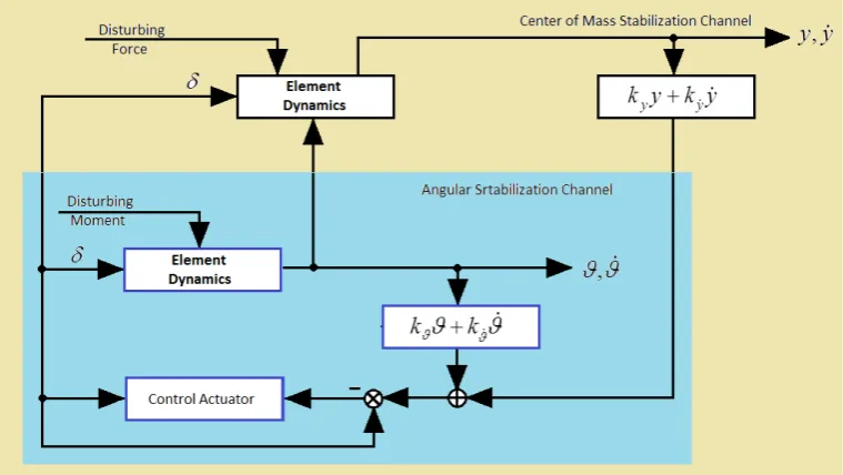
Figure 1. Functional diagram of model spacecraft stabilization

Objectives: to solve the task of significant increase in stabilization accuracy of centre of mass tangential velocities during the trajectory correction phases when using the "rigid" trajectory control principle.

Since the time of the active phase in correction manoeuvres, which is to be determined by the required velocity impulse, shall not be clearly determined in advance, and quite limited, and because a guaranteed approach enabling to estimate the accuracy, is always used in practice for solving the targeting tasks, we shall understand the maximum dynamic error of the transition process as concerns the drift velocity of the spacecraft to mean the accuracy of the spacecraft centre of mass movement stabilization [9].

Subject of research: The centre of mass movement stabilization system in the transverse plane, which is used during the trajectory correction phases.

In order the control actions could be created during the spacecraft trajectory correction phase, a high-thrust service propulsion system with a tilting or moving in linear direction combustion chamber shall be used.

Functioning of the spacecraft movement stabilization channel in the transverse plane is based on the feedback principle, and together with the spacecraft this channel forms a closed deviation control system. We can consider two channels in this control system: an angular stabilization channel and centre of mass movement stabilization channel (Fig. 1).

The angular stabilization channel facilitates angular position of the spacecraft when exposed to disturbing moments. The centre of mass movement stabilization channel is to ensure proximity to zero of normal and lateral velocities of the spacecraft under the influence of disturbing moments and forces. In most of the known (model) spacecraft stabilization systems [10-12] the control signal in the centre of mass movement stabilization channel is generated according to proportional plus integral control law

based on the measurements of tangential velocity of the centre of mass y z ( ) and its integral-linear drift y z( ). In the angular stabilization channel, the control signal shall be generated in proportion to the spacecraft deviation angle in the transverse plane

ϑ ψ

( ) and the angular velocity of the spacecraft rotation in this plane

ϑ ψ

 ( ).

The required dynamic accuracy of stabilization of tangential velocities in this system shall be achieved through the choice of the gain in the stabilization controller

, , , .

y y

k k k k ϑ ϑ If the requirements to the accuracy of centre

of mass movement stabilization are stiff, the coefficients ky

and ky shall be necessarily significantly increased [10].

However, if these coefficients are increased up to desired saturation, the system shall loose its motion stability, and further improvement of the accuracy of the spacecraft centre of mass movement stabilization shall be impossible when this method of control is applied. This can be explained by the fact that the increase in the gain values in the centre of mass movement stabilization channel results in improved performance of the channel, and the frequencies of the processes occurring in it become close to the frequencies of the angular stabilization channel, which fact enhances interaction of these two channels and makes it impossible to significantly improve the stabilization accuracy of the spacecraft centre of mass tangential velocities in the control system concerned.

of the propulsion system. This algorithm is based on the assumption that eccentricity and thrust misalignment in PS change slightly towards the end of the active phase during the previous correction, and PS setting before a new active phase sets in progress, ensures that the thrust vector goes approximately through the centre of mass of the spacecraft, thereby considerably offsetting the disturbing moment.

A similar algorithm was applied in the stabilization system of the Apollo spacecraft [14]. For its implementation, the control system was complemented with a so-called compensation circuit of thrust misalignment influence. The purpose of the referred circuit was to form a component to offset the total control signal so that the thrust vector could pass approximately through the centre of mass at zero output signals from the correction filter.

The stabilization systems of Titan IIIC, Kosmos-3M launchers also used subsystems tracking the centre of mass positional history, and providing the thrust vector's passage through the centre of mass [15].

It should be pointed out that the process of implementation of the described algorithm is confronted by a number of challenges [16]:

• Difference in disturbing factors (moments and forces) during the previous and subsequent corrections results in additional errors in the stabilization of the tangential velocities of the spacecraft centre of mass.

• Due to the limited time of the active phase, deactivation of PS during the previous correction may occur even before the completion of the transition processes in the stabilization system, and as a result, the system will remember the deviation of the steering control, which was not final.

Besides introduction of additional control algorithms, there are other ways to increase the accuracy of the centre of mass movement stabilization. It is a commonly known fact that one of the ways to achieve high accuracy in automatic control systems, is to use the so-called invariant theory [17-19]. The theory was developed by G.V. Shchipanov (1939), a Soviet scientist, who formulated the task "on compensation of external disturbances" [20]. Now, thanks to research conducted by the Soviet scientists G.V. Shchipanov, B.N. Petrov, V.S. Kulebakin, A.I. Kukhtenko and others the invariant theory represents a developed approach in the general theory of automatic control [16].

One of the problems inherent in the synthesis of invariant control systems, is the ability for the implementation of such systems in most cases through the use of the deviation control principle, as the simplest one and most widely used in practice. The publications [21-24] consider the possibility of constructing an invariant deviation control system with one adjustable parameter including an inertial element and a servo control with feedback. The general provisions of the invariant theory prove that no absolutely invariant system can be implemented in this case because this requires that the circuit with feedback should have an infinitely great gain.

As a rule, most invariant control systems are based on the use of the information about external influences. Such

control systems belong to the class of combined regulatory systems. In particular, the combined systems constitute the majority of invariant systems [25-31].

There is still another method to enforce implementation of invariance conditions without application of combined regulatory techniques [32]. This method is based on the dual-channel principle, which means that in order to ensure the absolute invariance of some adjustable value towards external influence, invariance with respect to the above influence should be ensured between the point of influence application and the measuring point. To implement such a system, it is necessary that two influence distribution channels should be present in the controlled element.

However, the referred task, i.e. stabilization of the spacecraft centre of mass movement in the active phase provides no possibility to measure disturbing influence, and the two influence distribution channels exist in the controlled element only for one of the disturbances, namely, for the disturbing moment. Therefore, this publication proposes a way to build a highly accurate stabilization system. We suggest that the requirements to comply with the conditions of invariance should be replaced with conditions of partial invariance when considering implementation of the invariance system. This method shall enable the synthesis of a highly accurate stabilization system, where the drift velocity of the spacecraft is a partially invariant value in respect to the disturbing moment and forces influencing the spacecraft in flight.

The concept of partial invariance in this case means that the invariance conditions for drift velocity shall be met regarding external influences themselves, and not their derivatives.

Meeting the conditions of partial invariance significantly reduces interaction between the angular stabilization channels and the centre of mass movement stabilization channel, which is present in the known (applied in practice) stabilization systems [15, 31, 33-38] and does not allow significant improvement of stabilization accuracy of the spacecraft drift velocity.

In order to improve the accuracy of the synthesized algorithms, we propose the application of self-configuring elements, which turn the operating device and X-axis of the spacecraft at angles recorded at the end of the previous active phase before a new active phase begins. The use of the above self-configuring elements in the synthesized invariant algorithms produces the maximum effect in increasing of the dynamic accuracy of tangential velocities stabilization as compared to similar techniques in the existing systems. This is due to the fact that the dynamic error of drift velocity in the synthesized algorithms, shall be largely determined by the initial conditions of the transition process due to the partial invariance of the algorithms proposed, which with the help of the mentioned self-configuring elements, can approach the values corresponding to the established mode as close as possible.

stability margins in partially invariant systems sufficient for practical implementation [16].

We propose an algorithm for selection of parameters of the stabilization controller, which facilitates minimization of maximum error during stabilization of the tangential velocity of the spacecraft centre of mass while ensuring adequate stability margins in the system.

2. Modeling of Transition Processes

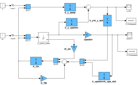
This chapter provides a description and results obtained from modelling of transition processes in a synthesized partially invariant centre of mass motion stabilization system of a spacecraft (Fig. 2) and, for comparison, in a stabilization system selected as a standard one (Fig. 3).

Figure 2. Block diagram of a partially invariant centre of mass stabilization system

The mathematical models of the stabilization systems employed take into account the following factors that were not considered in the system synthesis:

• PS servo control: The availability of a saturation zone and of a dead zone in the velocity performance of the control actuator, current amplification time constant in the control actuator, 'shunt running' operating device due to feedback interruption in the control actuator. • Angular Stabilization Channel: Signal lag due to the

presence of a filter in the output of the angular velocity sensor, numerical difference errors in angular speed, random interference (noise) in the angular speed sensor exit.

• Disturbing effects: Alteration of disturbing effects due to start of PS, accidental alteration of disturbing effects during normal operation of PS.

Now let's study components of the mathematical model of a partially invariant system closer.

• The controlled object: The movement of a spacecraft in a normal plane is described by four differential equations of the first order:

,

M

y y y F

d dt

d _{C C}

dt

dy y dt

dy C C C

dt ϑδ ϑδ ϑ δ δ

ϑ ϑ

ϑ

_δ

_δ

ϑ

δ

δ

 ₌    _{= − +}    ₌    _{= + +}      (1)

where

δ δ

M, F − are disturbances specified in the

equivalent PS deviation angles. The characteristics of the test spacecraft shall be the values of the dynamic coefficients:

2 2

1

13.2 ; _y 0.23 m .

C C C

s s grad

ϑδ = ϑ = ϑδ = _⋅

• PS servo control: PS servo control consists of a control actuator with an open feedback (in compliance with invariance requirements) and of a current amplifier for the control actuator. The velocity performance of the control actuator has a dead zone and a saturation zone. Deviation of the operating device has limits 60 on both sides from the neutral position. The current amplifier of the control actuator has a lag equal to 0.01 s. The broken feedback of the control actuator may result in the so-called 'shunt running' (a spontaneous deviation) of the control actuator. In the model, this factor shall be taken into account by supply of a continuous signal to input of the control actuator, which is 5 per cent of the value of the velocity performance saturation current in the control actuator. Consequently, PS servo control can be described by the following differential equations:

0

0

0

0 0

1 ( )

0, ,

( ),

( 0.05 )

, 6

6 ( ), 6

y

c y

c

c

c c c N

N c N c

OD c N

dI

K u I dt T

I I

I I I I I

I sign I I I

d _{K I I}

dt sign

δ

δ δ

δ

δ δ

= −  ≤ 

′ =_ < <

 _≤  ′ ′ = +  ′ ′ ≤  = 

′ ′ > 

(2)

here Tc− is a time constant of the current amplifier; Kc−

is a current amplifier coefficient; u− is control voltage signal in the output of the stabilization controller; Ic− is

amplifier-exit amperage; I I0, N − is dead band current and

saturation current of the control actuator velocity performance. The following values are taken to simulate performance of the servo control: Tc =0.01 ;s Kc =1

µ

_VA;

0 3 ;

I =

µ

A IN =40 ;

µ

A KOD =0.5grad_{s A}

_µ

.

• Stabilization controller: Pursuant to invariance and stability conditions obtained from the synthesis of the invariant system, a stabilization expression shall be as follows: u k= ϑ

ϑ

+kϑ

ϑ

+k y k yy+ y.

However, the expression above does not take into account several factors which, in the actual implementation of the system in question, can have a significant impact on the stabilization process, so they are to be taken into consideration when making a model. One such factor is that the second spacecraft angular deflection derivative

ϑ

 has to be obtained by numerical differentiation of the signal from the angular velocity sensor (AVS) performed by the on-board computer.

As a result of this differentiation, computational errors occur. In addition, calculation of the second angular derivative in the on-board computer results in delayed signals in the angular stabilization channel.

AVS output signal interruptions (noise) may significantly influence the stability of the system in question, as the interruptions increase manifold during the signal differentiation. In practice, in order to partially suppress AVS exit interruptions, we use an analogy filter, which may be described by an aperiodic link of the first order with a time constant TF. However, such a filter produces signal

delay in the angular stabilization channel in addition to interruptions reduction, thereby worsening the system's stability.

(

)

( ) ( 1)

1

1 _{( )}

F

AVS F

F

i i

F F

F y y

du _{K u}

dt T u u

u k k u k y k y

T ϑ ϑ ϑ

ϑ ξ

− = + −  −  =  + + +           (3)

where uF − is AVS filter exit signal; KAVS − is AVS

amplification factor;

ξ

ϑ− is AVS signal random error

(interruption); TF− is AVS filter time constant; ( )i _, ( 1)i

F F

u u − _{− are AVS signal values in the current and} previous steps in calculation of a derivative from the angular velocity by the on-board computer; T1− is a step in

calculations of angular velocity derivative.

The following values of the above characteristics were selected for modelling: KAVS =1_gradV s⋅ ; TF =0.01 ;s

1 0.01 ;

T = s k _{14 ;}s k _{6 ;}s k_{y 40}V s_;k_{y 80}V s2_.

m m

ϑ ϑ

⋅ ⋅

= = = =

   

The AVS signal error

ξ

_ϑ is considered to be Gaussian

uncorrelated random value, with a zero mathematical expectation and mean square deviation (MSD)

0.01grad.

s

ϑ

ξ

σ

_ = The MSD value was chosen from the condition that the accuracy of modern AVS is about one hundredths degree per second. The values of the stabilization controller coefficients k k k kϑ, , ,ϑ y y were selected based

on the author's algorithm.

• Disturbing effects. In the model (Fig. 4), the destabilizing force and disturbing moment shall be specified in the form of equivalent deviations of the operating device

δ δ

F, M at the exit of the

corresponding elements. This takes into account disturbance changes at the moment PS starts. For high-thrust space chemical engines, normal operation mode shall be activated during the lag time Tl ≈0.2 .s

During "software" PS launches [39], thrust and therefore, disturbance values connected with PS operation, shall change nearly linearly from zero to those corresponding to the normal PS operating mode. In the active phase, after PS enters normal operation mode, there are slight random fluctuations in the PS operation characteristics as compared to their nominal values, which shall in its turn affect the behaviour of the disturbing effects.

Therefore, in models, disturbances shall be specified as a relatively slow changing time function, randomly fluctuating relative to a specific value (mathematical disturbance expectation). The disturbances

δ δ

F, M _{appear as Gaussian}

stationary processes with mathematical expectations

,

F M

m m and correlation functions ( )( ) 2F M_{( )} k,

T F M

k e

τ

τ

=

σ

−

where

σ σ

F, M − is a mean square deviation of the

destabilizing force and disturbing moment in the equivalent angles of the operating device; T_k − is a constant, which characterizes disturbance modifications.

According to [39-42], the correlative function described above has a correspondent stochastic equation or a generating filter equation of the first order:

(

)

( )

( ) ( ), ,

F M

F M F M

d

a b m N

dt ξ

δ

δ

ξ

= − + (4)

where 1 , F M_{( )} 2

k k

a b N

T T Nξ ξ

σ

= = − is intensity of the white noise.

The mathematical expectations of the disturbing effects shall be determined by changing PS parameters in the normal operation mode. , _, , , , , H H l l F M l H H

m F m M t with t t t

m m

t t with m F m M

 <  =  _≥   (5)

where _{m F m M const}H , H _{= − are the mathematical}

expectations disturbances in the normal operation mode of PS.

The following values of the disturbance characteristics were selected for modelling: Tk =0.1 ;s

σ

F =0.1 ;0

0

0.3 ;

M

σ

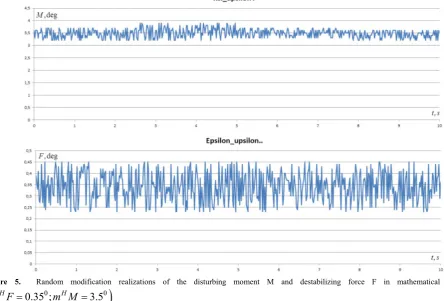
= _0.10_{≤m F}H _{≤0.35 ;0.3}0 0_{≤m M}H _{≤3.5 .}0

Fig. 5 shows how disturbing effects may be realized as accidental processes.

Thus, a structural scheme of a partially invariant stabilization system used in the modelling and taking into account the expressions (1-4) shall be as follows (Fig. 6). The response functions of generating filters M, F

ff ff

W W according (4) shall be as follows: ( )_{( ) ,}

1 ff F M ff ff K W S T S = +

where Kff =b_a,Tff =1_a.

The modelling was done by numerical integration of the equations (1-5) with application of Runge-Kutt 4th order method, with a controlled step size. Random values were modelled with application of Gaussian pseudo-random number sensors.

The integration of equations (1-5) was carried out within the time interval t=10 .s During the integration, the maximum drift velocity ymax, was recorded, which,

according to the task in question, is an indicator of the accuracy of the system. As ymaxis a random value because

of the randomness of the disturbances, we calculated the mathematical expectation my_maxof this parameter and its

MSD

σ

ymax considering 50 realizations of the stabilization

Figure 4. Signal indicating AVS error

ξ

_ϑ and the relative signal error in the derivative of angular velocity

ε

_ϑ as compared to the true value

_ϑ



Figure 5. Random modification realizations of the disturbing moment M and destabilizing force F in mathematical modelling

Figure 6. Block diagram of a partially invariant centre of mass stabilization system used in the mathematical modelling

In order to do a comparative analysis of the stabilization accuracy in the invariant and in standard stabilization systems, similar mathematical modelling was done for the standard system as well. As appears from the block diagram (Fig. 3), presence of control actuator feedback and a different stabilization controller distinguishes a model of the standard stabilization system from the model of the invariant system. Therefore, the expressions (2) and (3) for the standard system shall be (6) and (7) respectively:

0

0

0

0 0

1 ( )

0, ,

( ),

( )

, 6

6 ( ), 6

y

c y

c

c

c c c N

N c N c

OD c BF

dI

K u I dt T

I I

I I I I I

I sign I I I

d _{K I K}

dt sign

δ

δ δ

δ

δ δ

= −  ≤ 

′ =_ < <

 _≤  ′ ′ = −  ′ ′ ≤  = 

′ ′ > 

(6)

(

)

1 _{( )}

F

AVS F

F

F y y

du _{K u}

dt T

u k k u k y k y

ϑ ϑ ϑ

ϑ ξ

ϑ

= + − = + + +      (7)

The following parameter values were used in the modeling: 10 ; 10 ; 10; 20 ; 40 .

deg deg

FB V V y V y Vs

K k k k k

m m

ϑ ϑ

= = _= = =

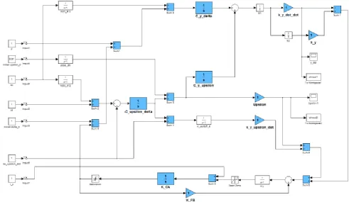
A block diagram for a model of the standard stabilization system used in the simulation is presented at Fig. 7.

Transition processes in the stabilization systems under consideration were modeled for zero initial conditions

(

0, , , , ,0 0 0 0 0

)

(

0,0,0,0,0,0 ,

)

T _T

y y

ϑ ϑ

 

δ δ

 = which are in line with the situation in which most of the known, practice-based stabilization systems operate. Also we modeled a system version, which used the suggested self-regulation elements, which involves setting of the initial values according to deviations of the operating device and of the body of the spacecraft recorded at the end of the previous active phase

(

0, , , , ,0 0 0 0 0

) (

,0,0,0, ,0 .

)

T T

f f

y y

ϑ ϑ  δ δ = ϑ δ

Let's consider and analyze modeling results in each of the cases described above.

3. Zero Initial Conditions Case

The results of the transition process modelling for the case of zero initial conditions are presented in Table 1 as mathematical expectation values mymax and the mean

square deviation

σ

ymax of the maximum drift velocity error

depending on the mathematical expectation of the disturbing effects H, H.

F M

m m

Also, it provides values for the following parameters describing the quality of the transition process: drift velocity damping amplitude during the period 1 2

1

,

C C C

ζ

= − _where

1, 2

C C − are drift velocity amplitudes at the beginning and at the end of the period; Tp− is oscillation period; T− is

transition process decay time. In order to assess the impact of accidental factors upon the stabilization accuracy, drift velocity stabilization error values y_max, calculated according to the deterministic model of the invariant stabilization system shall be given.

Table 1. Mathematical expectations and MSD of the drift velocity maximum error in the invariant and standard stabilization systems in zero initial conditions

,deg

H F

m 0.1 0.3 0.3 0.35

,deg

H M

m 0.3 1.0 2.0 3.5

max, ,m

y s

 invariant system 0.08 0.25 0.44 0.78

max, ,

y m

m s

 invariant system 0.07 0.25 0.47 0.8

max, ,

y v_s

σ

_ invariant system 0.03 0.03 0.02 0.03

max, ,

y m

m s

 standard system 0.21 0.59 1.07 1.82

max, ,

y v_s

σ

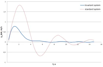
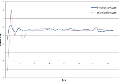
_ standard system 0.06 0.05 0.05 0.07

Figure 8. Spacecraft drift velocity transition processes in the normal plane in the invariant and standard stabilization systems (m_FH =0.3deg; m_MH =3.5deg)

Figure 10. Spacecraft X-axis deflection rate transition processes in the normal plane in the invariant and standard stabilization systems (m_FH =0.3deg; m_MH =3.5deg)

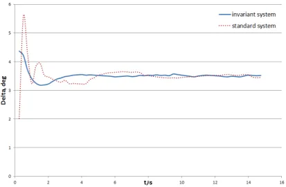
Figure 11. Operating device angular deviation transition processes in the normal plane in the invariant and standard stabilization systems (m_FH =_0.3deg; m_MH =_3.5deg)

As the mathematical modelling shows, application of the invariant algorithm in this case improves the accuracy of centre of mass roll stabilization twice or three times. Transition processes in the invariant stabilization system have significantly less attenuation time than in the standard

4. Self-Regulation Elements Version

In this case, modelling was like in the previous case, the difference being that the initial values were set non-zero

0, ,0

δ ϑ

that is we simulated initial OD and spacecraft X-axis alignment based on result of the previous adjustment (Table 2). The corresponding parameter values at the end of the transition processes were used as values

δ ϑ

0, 0 for the

case of non-zero initial conditions with correspondent

, .

H H

F M

m m Because in practice similar OD alignment shall be done with an error, which is approximately 30% of the true value, we used values

δ ϑ

0, 0 with 30% margin of error

in the mathematical modelling as well (See Fig. 8 – 15). Transition process diagrams for the invariant and standard stabilization systems are shown in Fig. 8 - 11 and correspond to maximum value case H, H.

F M

m m

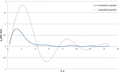
Based on the presented results, we can conclude that the accuracy of the invariant stabilization system increases significantly and is 4-5 times higher than the accuracy of a typical stabilization system, if self-regulation elements are used, providing similar self-regulation elements are used.

Table 2. Mathematical expectations and MSD of the drift velocity maximum error in the invariant and standard stabilization systems using self-regulation elements

,deg

H F

m 0.1 0.3 0.3 0.35

,deg

H M

m 0.3 1.0 2.0 3.5

max, ,m

y s

 invariant system -0.21 -0.73 -0.42 -2.45

max, ,

y m

m s

 invariant system 0.27 0.81 1.86 2.72

max, ,

y v_s

σ

_ invariant system -0.21 -0.73 -1.42 -2.45

max, ,

y m

m s

 standard system 0.07 0.13 0.18 0.28

max, ,

y v_s

σ

_ standard system 0.01 0.02 0.01 0.02

Figure 12. Spacecraft drift velocity transition processes in the invariant and standard stabilization systems

0 0

( H 0.3deg; H 3.5deg; 2.45deg; 2.75deg)

F M

Figure 13. Spacecraft X-axis angular deviation transition processes in the normal plane in the invariant and standard stabilization systems

0 0

( H 0.3deg; H 3.5deg; 2.45deg; 2.72deg)

F M

m = m =

ϑ

= −

δ

=

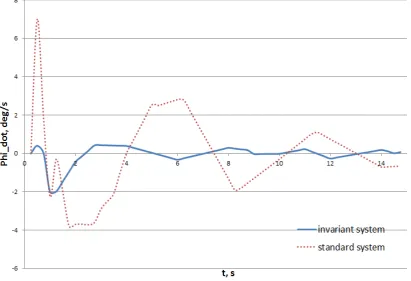
Figure 14. Spacecraft X-axis deflection rate transition processes in the normal plane in the invariant and standard stabilization systems

0 0

( H 0.3deg; H 3.5deg; 2.45deg; 2.72deg)

F M

Figure 15. Operating device angular deviation transition processes in the normal plane in the invariant and standard stabilization systems

0 0

( H 0.3deg; H 3.5deg; 2.45deg; 2.72deg)

F M

m = m =

ϑ

= −

δ

=

5. Conclusions

Based upon research results we can conclude the following:

1. It is impossible to implement a centre of mass stabilization system, which is absolutely invariant regarding both the disturbing force and disturbing moment.

2. In practice, a stabilization system, which is partially invariant to the disturbing moment M is the easiest to implement. In order to comply with the invariance conditions, there must be a positive control actuator feedback with a gain equal to the object's angular deflection gain of in the angular stabilization channel. Stability of the system shall be ensured by introduction of an additional second derivative action from the object's deflection angle into the action as well as by introduction of an equivalent delay loop in the feedback of control actuator in order to compensate for the dynamic delay of the stabilization controller.

3. It is also possible to synthesize a stabilization system, which shall be partially invariant fewer than two disturbances simultaneously. Open feedback of the control actuator and exclusion of control according to object's deflection angle and of the spacecraft centre of mass drift coordinate from the angular stabilization channel are the invariance conditions in this case Such a stabilization system has obvious advantages over a

system, which is invariant under disturbing moment M, and therefore it is more suitable for practical implementation.

4. A partially invariant fewer than two disturbances stabilization system provides a significant increase (several times) in the accuracy of the centre of mass tangential stabilization velocities as compared to known stabilization systems.

5. The tangential velocity transition process in a partially invariant stabilization system has a significantly shorter (several times) decay time as compared to known stabilization systems.

6. Employment of additional self-regulation elements in a partially invariant stabilization system reveals the significant advantages of such a system in terms of greater accuracy when compared to known stabilization systems.

REFERENCES

[1] Deep Impact Launch, 2005, Press Kit, January, NASA, USA. [2] H. B. William. 2005, Deep Impact Mission Design, Springler,

Space Science Reviews, 23-42.

[3] M. Taylor. 2011, The Rosetta mission, ESA.

[5] Zosimovych N., 2017, Modeling of Spacecraft Centre Mass Motion Stabilization System. International Refereed Journal of Engineering and Science (IRJES), Volume 6, Issue 4, 34-41.

[6] M.Y. Yamamoto. 2017, Observation plan for Martian meteors by Mars-orbiting MMX spacecraft. April, 11, [Online]. Available: https://www.cosmos.esa.int/documents/ 653713/1000951/01_ORAL_Yamamoto.pdf/c0143f57-5863-46da-bc00-e32e88be08a6.

[7] Yu. A. Surkov, R.S. Kremnev. 1998, Mars-96 mission: Mars exploration with the use of penetrators, ELSEVIER, Planetary and Space Science, Vol. 46, Issues 11-12, 1689-1696.

[8] 1996 Mars Mission, 1996, Press Kit, November, NASA, USA, 61 p.

[9] Zosimovych N. 2017, Improving the Spacecraft Center of Mass Stabilization Accuracy, IOSR Journal of Engineering (IOSRJEN), Vol. 7, Issue 6, 7-14.

[10] М.Н. Красильщиков, Г.Г. Себряков. 2003, Управление и

наведение беспилотных маневренных летательных аппаратов на основе современных информационных технологий. М.: ФИЗМАТЛИТ, 280 с.

[11] А.А. Лебедев, В.Т. Бобронников, М.Н. Красильщиков и

др. 1985, Статистическая динамика и оптимизация управления летательных аппаратов. М.:

Машиностроение, 280 с.

[12] Г. Стаббс, А. Пинчук, Р. Шлюндт, 1970, Цифровая Система стабилизации космического корабля “Аполлон”. – Вопросы ракетной техники, No 7.

[13] В.К. Абалакин, Е.П. Аксенов, Е.А. Гребеников и др., 1976, Справочное руководство по небесной механике и астродинамике. M: Наука, 864 с.

[14] R.G. Chilton. 1965, Apollo Spacecraft Control Systems. NASA Manned Spacecraft Control Houston, Texas, USA. [15] N. Zosimovych. 2016, Commercial Launch Vehicle Design,

LAP LAMBERT Academic Publishing, 184 p.

[16] J.W. Polderman, J.C. Willems. 2008, Introduction to Mathematical Systems Theory: A Behavioral Approach (Texts in Applied Mathematics), Springer; 2nd edition, 455 p. [17] Spasskii R.A. 1992, Invariance of a system of automatic

control, Journal of Soviet Mathematics, June, Volume 60, Issue 2, PP. 1343–1346.

[18] Bamieh B., Paganini F., Dahleh M.A. 2002, Distributed Control of Spatially Invariant Systems, IEEE Transactions on Automatic Control, Vol. 47, No. 7, July, PP. 1091-1107. [19] Щипанов Г.В. 1939, Теория и методы проектирования

автоматических регуляторов, Автоматика и телемеханика, № 1.

[20] А.И. Репин. 2011, Теория автоматического управления (Конспект лекций), Можайск, 150 с.

[21] Бейнарович В.А. 2010, Инвариантные системы

автоматического управления с релейным усилителем, Доклады ТУСУРа, №2 (21), Часть 1, Июнь, СС. 70-73. [22] R.C. Dorf, R.H. Bishop. Modern Control Systems, Pearson,

12th _{edition, 807 pp.}

[23] Ferrari S., Stengel R.F.. 2004, Online Adaptive Critic Flight Control, Journal of Guidance, Control, and Dynamics, Vol. 27, No 5, September-October, pp. 777-786.

[24] The Electronics Engineer’s Handbook. 2005, 5ty Edition McGraw-Hill 19, pp. 19.1-19.30.

[25] J.W. Polderman, J.C. Willems. Introduction to the Mathematical Theory of Systems and Control, 458 pp. [26] E. Feron, G. Brat, P.L. Garoche, P. Manolios, M. Pantel. 2012,

Formal methods for aerospace applications. FMCAD tutorials.

[27] M. Colon, S. Sankaranarayanan, H.B. Sipma. 2003, Linear invariant generation using non-linear constraint solving. In Proc. CAV, LNCS, pp. 420-432. Springler.

[28] Souris J., Favre-Felix D.. 2004, Proof of properties in avionics. In Building the Information Society, Vol. 156, pp. 527-535. Springler.

[29] J.C. Hennet, D.C.E. Trabuco. 1994, Invariant Regulators for Linear Systems under Combined Input and State Constraints. Proc. 33rd _{Conf. of Decision and Control (IEEE-CDC’94),}

Lake Buena Vista, Florida USA, Vol. 2, pp. 1030-1036. [30] A. Luca, P. Rodriguez, D. Dumur. 2009, Invariant sets

method for state-feedback control design, 17th

Telecommunications forum TELEFOR Serbia, Belgrad, November 24-26, PP. 681-684.

[31] G. Rustamov. 2012, Invariant Control Systems of Second Order, IV International Conference “Problems of Cybernetics and Informatics” (PCI’2012), September 12-14, Baku, PP. 22-24.

[32] A. Kelly. 1994, Modern Inertial and Satellite Navigation Systems. The Robotics Institute Carnegie Mellon University, CMU-RI-TR-94-15.

[33] M. Horemuž. 2006, Integrated Navigation. Royal Institute of Technology, Stocholm.

[34] V.V. Malyshev, M.N. Krasilshikov, V.T. Bobronnikov, V.D. Dishel. 1996, Aerospace vehicle control, Moscow, MAI. [35] P. Albertos, A. Sala. 2004, Multivariable Control Systems,

Valensia, Spain.

[36] B. Averil. 1997, Chatfield Fundamentals of High Accuracy Inertial Navigation. Vol. 174, Progress in Astronautics and Aeronautics.

[37] V.M. Sineglazov. 2003, Theory of automatic control. In 2 Vol.: Manual for students of all specialities, Kyiv, NAU. [38] A Review of United States Air Force and Department of

Defense Aerospace Propulsion Needs, 2006, The National Academies Press, Washington D.C., 90 p. [Online]. Available: www.nap.edu.

[39] А.А. Лебедев, Г.Г. Аджимамудов, В.Н. Баранов, В.Т. Бобронников и др. 1996, Основы синтеза систем летательных аппаратов. М.: МАИ, 224 c.

[41] J. Piovesan, Ch. Abdallah, M. Egerstedt, H. Tanner, Y. Wardi. 2007, Statistical Learning for Optimal Control of Hybrid Systems. American Control Conference, ACC '07, 9-13 July, IEEE.