Chaos-Based Image Encryption Using an
Improved Quadratic Chaotic Map
Noha Ramadan1,*, Hossam Eldin H. Ahmed1, Said E. Elkhamy2, Fathi E. Abd El-Samie1
1
Communication, Faculty of Electronic Engineering, Menofia University, Egypt
2
Electrical Engineering, Faculty of Engineering, Alexandria University, Egypt
Abstract
In recent years, chaos-based image encryption has become an efficient way to encrypt images due to its high security. In this paper, we improve the classical Quadratic chaotic map to enhance its chaotic properties and use it for image encryption. Compared with the classical Quadratic map, the proposed Quadratic map demonstrates better chaotic properties for encryption such as a much larger maximal Lyapunov exponent. The proposed image encryption scheme is based on two chaotic maps. The first map is the Chepyshev chaotic map, which is used for the permutation of the pixels of the image. The permuted image is subjected to the diffusion process using the improved Quadratic map in an efficient encryption algorithm which its key is related to the original image. The main advantages of the proposed scheme are the large key space and its resistance to various attacks. Simulation results show that the proposed scheme has a high security level with low computational complexity, which makes it suitable for real-time applications.Keywords
Chaos encryption, Quadratic map, Chepyshev, Lyapunov exponent1. Introduction
In recent years, the transmission of a large amount of data such as video conferences, medical and military images over communication media was highly developed. The security of information transmitted is a vital issue. Most conventional secure ciphers such as Data Encryption Standard (DES) [1] and Advanced Encryption Standard (AES) [2] are not suitable for fast encryption of a large data volume in real time. The implementation of traditional algorithms for image encryption is even more complicated because of the high correlation between image pixels. Therefore, there is still a lot of work to be done for the development of sophisticated encryption methods. Many researchers have pointed out the existence of a strong relationship between chaos and cryptography. The idea of using chaos in cryptography can be traced back to Shannon on secrecy systems [3]. Although the word "chaos" was not minted till the 1970s [4], the use of chaos in cryptography seems quite natural. The two basic properties of a good cipher; confusion and diffusion are strongly related to the fundamental characteristics of chaos such as a broadband spectrum, ergodicity and high sensitivity to initial conditions. The implementation of Shannon's idea had to wait till the development of chaos theory in the 1980s.
* Corresponding author:
[email protected] (Noha Ramadan) Published online at http://journal.sapub.org/ajsp
Copyright © 2016 Scientific & Academic Publishing. All Rights Reserved
In the first scientific paper on chaotic cryptography that appeared in 1989, Matthews [5] came up with the idea of a stream cipher based on one-dimensional chaotic map. Afterwards, chaotic cryptography has spread and more papers about digital chaotic ciphers have been published [6-8].
Traditionally, encryption is based on discrete number theory, so that data has to be digitized before any encryption process can take place. In order to encrypt a continuous voice or a video in the old fashion, digitalization and encryption can pose a heavy computational process. The use of chaotic communication enables to encrypt the message waveform without a need to digitalize it [9].
Based on strengths and weaknesses of already existing algorithms, Kelber and Schwarz formulated several general rules to design a good chaos-based cryptosystem [9-10]:
Either use a suitable chaotic map, which preserves important properties during discretization for block cipher or use a balanced combining function and a suitable key-stream generator for a stream cipher. Use a large key space.
Avoid simple permutations of identical system
parameters.
Use the same precision for sub-key values and their corresponding system parameters.
Use a complex input key transformation.
Use a dynamical system.
Use complex nonlinearities.
Modify nonlinearities in terms of key and signal
Use several rounds of operation for block ciphers. The basic properties of chaotic systems are the deterministicity, the sensitivity to initial conditions and parameters and the ergodicity. Deterministicity means that chaotic systems have some determining mathematical equations ruling their behavior. The sensitivity to initial conditions means that when a chaotic map is iteratively applied to two initially close points, the iterations quickly diverge, and become uncorrelated in the long term. Sensitivity to parameters causes the properties of the map to change quickly, when slightly disturbing the parameters, on which the map depends. Hence, a chaotic system can be used as a pseudo-random number generator. The ergodicity property of a chaotic map means that if the state space is partitioned into a finite number of regions, no matter how many, any orbit of the map will pass through all these regions.
A number of traditional chaotic maps such as Quadratic map [11] and Logistic map [12] have limited properties and may no longer satisfy our needs. Without improvement of chaotic maps, our applications will remain unchanged and might be subject to different attacks in the future. Hence, there is a bad need for more improvements in the chaotic maps.
In this paper, an improved Quadratic chaotic map is first introduced. We use the maximal Lyapunov exponent [13] and the bifurcation diagram to determine the performance of the map. A new image encryption scheme based on this improved Quadratic map is presented containing two main processes; permutation and diffusion. The permutation process breaks the strong relationship between adjacent pixels. The permutation operation only shuffles the pixel positions without changing values. The shuffled and original images have the same entropy, and therefore the shuffled image is weak against statistical attack and known plain-text attack.
In the diffusion process, the pixel values are altered. Most researchers focus on security improvements [14-15], while only a few are dealing with efficiency issues [16-17]. For most of the security improvements, researchers need at least three rounds of the diffusion process to obtain a satisfactory
performance. Researchers focusing on efficiency
improvement only need one round of the diffusion process to achieve the high security level and speed up the performance. However, some of the proposed algorithms lead to a longer processing time in a single round. Therefore, the key problem of designing an efficient image cryptosystem is how to reduce the computational complexity with efficiently to avoid the large number of rounds in the generation of diffusion and permutation keys and then achieve high speed performance. At the permutation step, we sort the chaotic sequences of the Chepyshev map in order to shuffle the entire image. At the diffusion step, the shuffled image is encrypted with a key related to plain image.
2. Analysis of Quadratic Map
Quadratic map is a basic example of a chaotic system. The equation of the classical Quadratic map is [18]:
xn+1= r – ( xn)2 (1)
where r is the chaotic parameter and n is the number of iterations. The system of the Quadratic map is chaotic, because it is nonlinear. It is deterministic since it has an equation that determines the behavior of the system. Also, a very slight change of the initial value x0can lead to a
significantly different behavior of the map. In the following subsections, many plots for the analysis of the Quadratic chaotic map will be studied such as the iteration property, the bifurcation diagram, and the Lyapunov exponent.
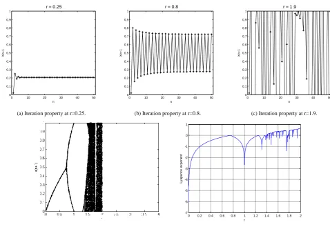
2.1. Iteration Property
The iteration diagram plots the relation between the number of iterations n and the Quadratic chaotic map at different values of the chaotic parameter r and at a specific initial value x0. The parameter r can be divided into three
regions, which can be examined by simulation using MATLAB as following:
When r[0,0.74], as shown in Fig. 1 (a), the calculated
value come to the same result after several iterations without
any chaotic behavior. When r[0.74,1.5], as shown in Fig.
1 (b), the system appears as having a periodic behavior.
When r[1.5, 2], it becomes a chaotic system as shown in
Fig. 1 (c).
2.2. Bifurcation Diagram
Bifurcation is usually referred to as the qualitative transition from regular to chaotic behavior by changing the
control parameter.The bifurcation diagram is used to study
the chaotic system as a function of the values of the control parameters. This diagram allows knowing the regions of the system displaying convergence, bifurcation, and chaos depending on the values of the control parameters [19].
Fig. 1 (d) shows the bifurcation diagram of the classical Quadratic map. This diagram has three regions. The
convergence region is at r[0,0.74]. The bifurcation
region is at r[0.74,1.5] . The chaos region is at
[1.5, 2]
r , where the chaotic behavior occurs.
2.3. Lyapunov Exponent
Lyapunov exponent represents the features of a chaotic system and can largely express the overall performance of chaotic maps. It is used as a quantitative measure for the sensitive dependence on initial conditions. For a discrete system xn+1 =f(xn) and for an orbit starting with x0, the
Lyapunov exponent can be defined as follows [20-21]:
λ (x0) = limn→∞1n ∞i=1 ln f′(xi) (2)
the system is not chaotic. If λ is zero, this means that the system is neutrally stable and is in steady state mode. If λ is positive, the evolution is sensitive to initial conditions and therefore chaotic. Also, it is common to refer to the largest defined by Eq.(2) as the Maximal Lyapunov Exponent (MLE), because it determines a notion of predictability for a chaotic system. The larger MLE is, the more chaotic the map is and the smaller the number of iterations necessary to achieve the required degree of diffusion or confusion of information is, and this means a better chaotic map.
Fig. 1 (e) shows the Lyapunov exponent of the classical
Quadratic map. It is obviously clear that when r[0,1.5],
all Lyapunov exponents are less than or equal to zero. When
[1.5,2]
r , the Lyapunov exponents are positive, and hence
chaotic. The maximal Lyapunov exponent of the Quadratic map is 0.6720.
3. The Proposed Quadratic Map
The equation of the proposed quadratic map is:
Xn+1 = (r+ (1-axn)2) mod 1 (3)
We will replace -(xn)2 in Eq.(1) with the term (1-axn)2 and
module 1. Now, we will examine the proposed Quadratic maps and plot the iteration property, bifurcation diagram,
and Lyapunov exponent at three different values of a = 2, 4, 8.
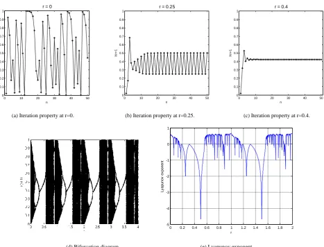
3.1. Analysis of the Proposed Quadratic Map 1
The equation of the proposed Quadratic map 1 at a= 2 is: Xn+1 = (r+ (1-2xn)2) mod 1 (4)
Fig. 2 shows the analysis of the proposed Quadratic map 1. From Fig. 2 (a), (b), (c), and (d), it is clear that there are several convergence, bifurcation, and chaos regions. These regions are extended to infinity. The bifurcation regions are at r[0.15, 0.31], r[1.15,1.31], etc…. to infinity. The
convergence regions are at r[0.31,0.56], r[1.2,1.56],
etc…. to infinity. The chaos regions are at r[0, 0.14],
[1.56, 2.14]
r , r[2.56, 3.14], etc…. to infinity, where the chaotic behavior occurs.
Now, it is obvious that the chaotic range of the proposed Quadratic map 1 is larger than the chaotic range for the classical one, and hence this will increase the available chaotic value of parameter r that can be used in encryption.
In Fig. 2 (e), the Lyapunov exponent has a positive value at r[0, 0.14], r[1.56, 2.14], r[2.56, 3.14], etc…, and hence the proposed Quadratic map 1 exhibits a chaotic behavior at these periods. The MLE of the proposed Quadratic map 1 is 0.6732, which is greater than the classical Quadratic map but still small.
0 10 20 30 40 50
0 0.1 0.2 0.3 0.4 0.5 0.6 0.7 0.8 0.9 1
r = 0.25
n
X
n
+
1
0 10 20 30 40 50
0 0.1 0.2 0.3 0.4 0.5 0.6 0.7 0.8 0.9 1
r = 0.8
n
X
n
+
1
0 10 20 30 40 50
0 0.1 0.2 0.3 0.4 0.5 0.6 0.7 0.8 0.9 1
r = 1.9
n
X
n
+
1
(a) Iteration property at r=0.25. (b) Iteration property at r=0.8. (c) Iteration property at r=1.9.
(d) Bifurcation diagram. (e) Lyapunov exponent.
Figure 1. Analysis of the classical Quadratic map at x0=0.02
0 0.2 0.4 0.6 0.8 1 1.2 1.4 1.6 1.8 2
-7 -6 -5 -4 -3 -2 -1 0 1
r
L
y
a
p
u
n
o
v
e
x
p
o
n
e
n
0 10 20 30 40 50 0
0.1 0.2 0.3 0.4 0.5 0.6 0.7 0.8 0.9 1
r = 0
n
X
n
+
1
0 10 20 30 40 50
0 0.1 0.2 0.3 0.4 0.5 0.6 0.7 0.8 0.9 1
r = 0.25
n
X
n
+
1
0 10 20 30 40 50
0 0.1 0.2 0.3 0.4 0.5 0.6 0.7 0.8 0.9 1
r = 0.4
n
X
n
+
1
(a) Iteration property at r=0. (b) Iteration property at r=0.25. (c) Iteration property at r=0.4.
(d) Bifurcation diagram. (e) Lyapunov exponent.
Figure 2. Analysis of the proposed Quadratic map 1 at x0=0.02 3.2. Analysis of the Proposed Quadratic Map 2
The equation of the proposed Quadratic map 2 at a= 4 is: Xn+1 = (r+ (1-4xn)2) mod 1 (5)
Fig. 3 shows the analysis of the proposed Quadratic map 2. From Fig. 3 (a), (b), (c), and (d), it is clear that the convergence and bifurcation regions have become very small and chaos regions are increased. These regions are extended to infinity. The bifurcation regions are at r[0.138, 0.14],
[0.17, 0.19]
r , r[1.138,1.14] , r[1.17,1.19]
etc…. to infinity. The convergence regions are at
[0.2,0.266]
r , r[1.2,1.266], etc…. to infinity. The
chaos regions are at r[0, 0.137] , r[0.14, 2.14],
[1.14,3.14]
r , etc…. to infinity, except the small regions
of convergence and bifurcation, where the chaotic behavior occurs.
In Fig. 3 (e), the Lyapunov exponent has a positive value at all values of r except small ranges of convergence and bifurcation. Hence, the proposed Quadratic map 2 exhibits a chaotic behavior in the rest of the range. The MLE
of the proposed Quadratic map 2 is 2.0257, which is much greater than the classical Quadratic map and proposed Quadratic map 1.
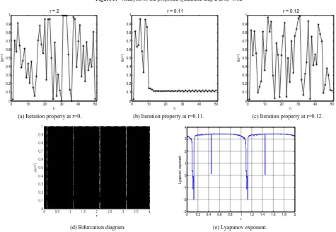
3.3. Analysis of the Proposed Quadratic Map 3
The equation of the proposed Quadratic map 3 at a= 8 is:
Xn+1 = (r+(1-8xn)2)mod 1 (6)
Fig. 4 shows the analysis of the proposed Quadratic map 3. From Fig. 4 (a), (b), (c), and (d), it is clear that the proposed Quadratic map 3 exhibits a chaotic behavior at all values of r except the values 0.11, 1.11, etc…. to infinity.
In Fig. 4 (e), the Lyapunov exponent has a positive value at all values of r except the values of 0.11, 1.11, etc…. So, the proposed Quadratic map 3 exhibits a chaotic behavior at the rest of the range. The MLE of the proposed Quadratic map 3 is 3.4709, which is much greater than the classical Quadratic map and the proposed Quadratic map 1 and 2.
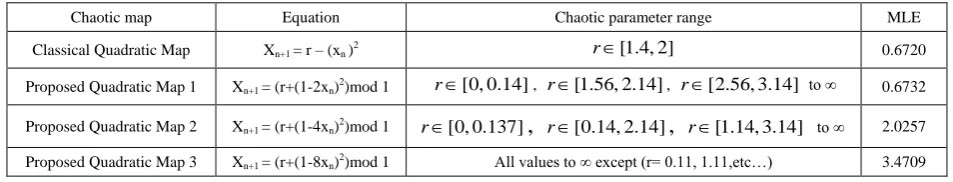
Table (1) summarized the analysis of the classical and proposed quadratic maps. It shows the improvement in both the chaotic parameter range r and MLE.
0 0.2 0.4 0.6 0.8 1 1.2 1.4 1.6 1.8 2
-5 -4 -3 -2 -1 0 1
r
L
y
a
p
u
n
o
v
e
x
p
o
n
e
n
0 10 20 30 40 50 0 0.1 0.2 0.3 0.4 0.5 0.6 0.7 0.8 0.9 1
r = 0
n
X
n
+
1
0 10 20 30 40 50
0 0.1 0.2 0.3 0.4 0.5 0.6 0.7 0.8 0.9 1
r = 0.18
n
X
n
+
1
0 10 20 30 40 50
0 0.1 0.2 0.3 0.4 0.5 0.6 0.7 0.8 0.9 1
r = 0.2
n
X
n
+
1
(a) Iteration property at r=0. (b) Iteration property at r=0.18. (c) Iteration property at r=0.2.
(d) Bifurcation diagram. (e) Lyapunov exponent.
Figure 3. Analysis of the proposed Quadratic map 2 at x0=0.02
0 10 20 30 40 50
0 0.1 0.2 0.3 0.4 0.5 0.6 0.7 0.8 0.9 1
r = 2
n
X
n
+
1
0 10 20 30 40 50
0 0.1 0.2 0.3 0.4 0.5 0.6 0.7 0.8 0.9 1
r = 0.11
n
X
n
+
1
0 10 20 30 40 50
0 0.1 0.2 0.3 0.4 0.5 0.6 0.7 0.8 0.9 1
r = 0.12
n
X
n
+
1
(a) Iteration property at r=0. (b) Iteration property at r=0.11. (c) Iteration property at r=0.12.
(d) Bifurcation diagram. (e) Lyapunov exponent.
Figure 4. Analysis of the proposed Quadratic map 3 at x0=0.02
0 0.2 0.4 0.6 0.8 1 1.2 1.4 1.6 1.8 2
-4 -3 -2 -1 0 1 2 3 r L y a p u n o v e x p o n e n t
0 0.2 0.4 0.6 0.8 1 1.2 1.4 1.6 1.8 2
Table (1). Comparison between the classical and proposed Quadratic maps
Chaotic map Equation Chaotic parameter range MLE
Classical Quadratic Map Xn+1 = r – (xn )2 r[1.4, 2] 0.6720
Proposed Quadratic Map 1 Xn+1 = (r+(1-2xn)2)mod 1 r[0, 0.14], r[1.56, 2.14], r[2.56, 3.14] to ∞ 0.6732
Proposed Quadratic Map 2 Xn+1 = (r+(1-4xn)2)mod 1 r[0, 0.137]
,
r[0.14, 2.14],
r[1.14, 3.14] to ∞ 2.0257Proposed Quadratic Map 3 Xn+1 = (r+(1-8xn)2)mod 1 All values to ∞ except (r= 0.11, 1.11,etc…) 3.4709
4. Application on Image Encryption
Now, we will introduce the proposed image encryption scheme based on two chaotic maps; the Chepyshev map and the proposed Quadratic maps we have just constructed.
4.1. Chepyshev Chaotic Map
The Chepyshev chaotic map is a one dimensional chaotic
system with one initial condition x0 and one control
parameter k and can be described as follows [22]:
yn+1 =cos (𝑘 cos-1 (y𝑛)) (7)
where yn [−1, 1] for n = 0, 1,2, … and k [2,∞). The
bifurcation diagram of the Chepyshev map in Fig. 4 shows that all the (y0, k) where y0 [-1, 1] and 2 ≤ k < ∞ can be
used as secret keys. The Chepyshev map has a positive increasing Lyapunov exponent at k >= 2, and thus, it is always chaotic as shown in Fig. 5.
Figure 4. Bifurcation diagram of the Chepyshev chaotic map at x0=0.02
Figure 5. Lyapunov exponent of the Chepyshev chaotic map
4.2. The Permutation Process
We use Chepyshev chaotic map to generate chaotic sequences x and then sort that chaotic numbers in ascending or descending order for the generation of the permutation
key. For a 256-level gray-scale image, y0= 0.97 and k= 2.995.
We sort the chaotic sequences in the index matrix used in shuffling the original image to obtain the permuted image. The original Cameraman image and the permuted image after permutation are shown in Fig. 7 and Fig. 8. After obtaining the shuffled image, the correlation among the adjacent pixels is completely disturbed and the image is completely unrecognizable. The histogram of the permuted image and the original image are the same, since there is no change in the intensity of pixels as shown in Fig. 9 and Fig. 10. Therefore, the permuted image is weak against statistical attack, and known plain-text attack. As a result, we employ a diffusion process after permutation to improve the security.
Figure 7. Original image
Figure 8. Permuted image
0 5 10 15
-1 -0.5 0 0.5 1 1.5 2 2.5 3
k
L
y
a
p
u
n
o
v
e
x
p
o
n
e
n
Figure 9. Histogram of the original image
Figure 10. Histogram of the permuted image
4.3. Image Diffusion Based on the Proposed Quadratic Chaotic Maps
The diffusion step in the proposed encryption scheme is performed by the key related to the plain image algorithm which used only one round diffusion operation and its key depends on the initial key and the original image [23]. We will use the proposed Quadratic maps and also the classical Quadratic map in the diffusion process and compare between them. After comparison, we will get the chaotic map which has the best performance. We will treat the image as a one
dimensional vector im = {im1, im2… imL} of length L= M×N.
The initial value x0 =0.02.
We will discuss the encryption process only, because the decryption is the reverse process. The details of the encryption process can be summarized as follows:
Step 1: for n =1, iterate the classical and proposed Quadratic maps using Eqs. (1), (4), (5) and (6) for only one time to get x1.
Step 2: modify x1 according to the following equation,
where im1 is any arbitrary image pixel.
x1= mod (x1+ (im1+ 1)/255,1) (8) Step 3: for n =n+1 return to step 1 until n=L to get xL.
Let the new initial value of the proposed Quadratic map 3 be (x0+xL)/2.
Step 4: iterate the proposed Quadratic map 3 using Eq. (8)
for L times with the new initial value. Then, we obtain the sequence.
X = xL+1, xL+2, … , x2L (9) Step 5: to get the sequence K= {k1, k2,…,KL} use
kn= mod floor xL+n×105 , 256 (10)
Where n = 1, 2, . . , L
Step 6: examine the randomness of the sequence kn:
H = runstest(kn) (11)
By using the Matlab function (runstest) for randomness, H returns (0) if the sequence is random and (1) if not. In our case, H=0.
Step 7: compute the first cipher pixel by using the value of im1, the constant c, and the first key k1.
c1= k1⨁mod im1+ c, 256 (12) Step 8: let n=n+1
Step 9: compute the nth pixel of the cipher image by using
the following equation in which the cipher output feedback is introduced.
cn= kn⨁mod imn+ imn−1, 256 (13) Step 10: repeat step 8 and step 9 until n reaches L, and then the cipher image C= {c1, c2,…,cn} is obtained.
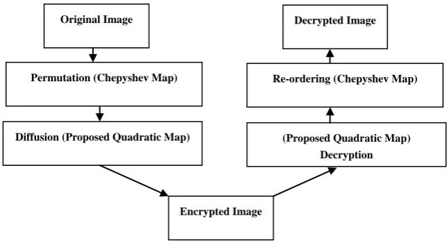
5. The Proposed Scheme
The proposed encryption scheme is based on a permutation-diffusion architecture. The first stage is applying the permutation process to the original image. Then, the permuted image is subjected to the diffusion process. The permutation is achieved using Chepyshev map. The diffusion process is achieved by the key related to the plain image algorithm based on the proposed Quadratic maps we have just constructed. The decryption process is simply the reverse of the encryption process. See Fig. 11.
6. Performance Analysis
The quality of the encryption algorithm is its ability to resist different kinds of known attacks such as known/chosen plain-text attack, cipher-text only attack, statistical attack, differential attack, and various brute-force attacks. We will examine the proposed algorithm by measuring security, statistical, and sensitivity analysis on different images.
6.1. Security Analysis
6.1.1. Key Space Analysis
The key space is the total number of different keys that can be used in the encryption process. The proposed algorithm consists of two processes; permutation and diffusion. In the permutation process, we use Chepyshev map with two
independent variables y0 and k. In the diffusion process, the
Quadratic map has two independent variables x0 and r. In the
key related to the plain text algorithm, we have a constant
0 50 100 150 200 250
0 100 200 300 400 500 600 700 800 900 1000
0 50 100 150 200 250
integer c and c [1, 255]. As a result, the key space is {y0, k,
x0, r, c}. Since y0, k, x0 and r are double precision numbers,
the total number of different values for y0, k, x0 and r is more
than 1014. So, the key space is larger than 1014 1014 1014 1014 255. This large key space is enough to resist brute-force attack. On the other hand, the key space of RC6, DES and chaotic Baker map for the same 256 level gray-scale image is 2128, 256,and 263 respectively [24]. See Table (2)
Table (2). The key space comparison
The encryption scheme The key space
The proposed hybrid chaotic scheme 10141014 10141014 255
RC6 2128
DES 256
Chaotic Baker map 263
6.1.2. Statistical Analysis
In order to prove the security of the proposed encryption algorithm, the following statistical tests are performed.
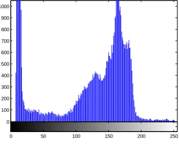
(a) Histogram
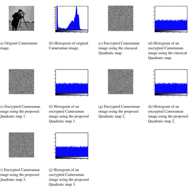
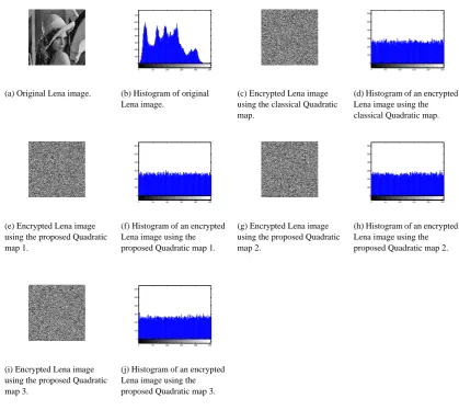
Histogram clarifies that how pixels in an image are distributed by plotting the number of pixels at each gray-scale level. The histogram of the original Cameraman, Mandrill and Lena images and their encrypted versions with the classical Quadratic map, the proposed Quadratic map 1, 2 and 3 are shown in Figs. 12, 13 and 14. These figures show that the histograms of the encrypted images of all Quadratic maps are fairly uniform and completely different from those of the original images.
(b) Correlation Coefficient
For an original image, adjacent pixels have a large correlation. For an encrypted image, the correlation between pixels should be as small as possible. The closer the value of correlation coefficient (CC) to zero, the better is the encryption. If the correlation coefficient equals zero, then the
original image and its encrypted version are totally different. So, the success of the encryption process means smaller values of the correlation coefficient. The CC is measured by the following equation [25]:
1
2 2
1 1
( ( ))( ( )) ( ( )) ) ( ( )) )
N
i i
i
N N
i i
i i
x E x y E y CC
x E x y E y
Where (
1
1
( ) N i
i
E x x
N
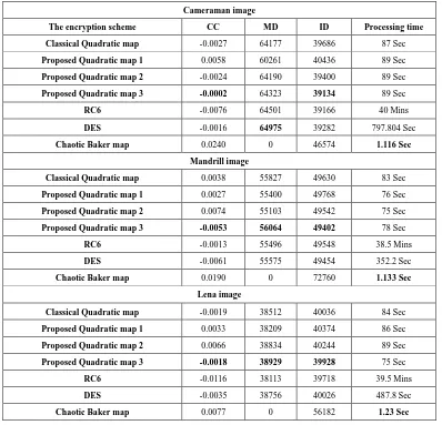
) (14)where x and y are the gray-scale pixel values of the original and encrypted images. Table (3) shows the CC of the proposed scheme using the classical and proposed Quadratic maps, RC6, DES and chaotic Baker map for different test images. The simulation results show that all the encryption algorithms listed have a very small CC, and the proposed scheme based on the proposed Quadratic map 3 has the best CC.
(c) Maximum Deviation
The Maximum Deviation (MD) measures the quality of the encryption in terms of how it maximizes the deviation
between the original and the encrypted images [26]. The
higher the value of MD, the more the encrypted image is deviated from the original image. Table (3) shows that the MD of the proposed scheme based on the proposed Quadratic map 3 is the highest compared to the classical and the proposed Quadratic maps 1, 2. The DES has the best MD for Cameraman image, only. The worst result of this test was found in the chaotic Baker chaotic with a result of zero, because this algorithm depends only on permutation.
(d) Irregular Deviation
The Irregular Deviation (ID) is based on how much the deviation caused by encryption is irregular [27]. The lower the ID value, the better the encryption algorithm. Table (3) shows that the ID of the proposed scheme with the proposed Quadratic map 3 has the smallest value for all tested images.
Figure 11. The proposed scheme
Original Image
Permutation (Chepyshev Map)
Diffusion (Proposed Quadratic Map)
Decrypted Image
Re-ordering (Chepyshev Map)
(Proposed Quadratic Map) Decryption
0 50 100 150 200 250 0
100 200 300 400 500 600 700 800 900 1000
0 50 100 150 200 250 0
100 200 300 400 500 600
(a) Original Cameraman image.
(b) Histogram of original Cameraman image.
(c) Encrypted Cameraman image using the classical Quadratic map.
(d) Histogram of an encrypted Cameraman image using the classical Quadratic map.
0 50 100 150 200 250 0
100 200 300 400 500 600
0 50 100 150 200 250 0
100 200 300 400 500 600
(e) Encrypted Cameraman image using the proposed Quadratic map 1.
(f) Histogram of an encrypted Cameraman image using the proposed Quadratic map 1.
(g) Encrypted Cameraman image using the proposed Quadratic map 2.
(h) Histogram of an encrypted Cameraman image using the proposed Quadratic map 2.
0 50 100 150 200 250 0
100 200 300 400 500 600
(i) Encrypted Cameraman image using the proposed Quadratic map 3.
(j) Histogram of an encrypted Cameraman image using the proposed Quadratic map 3.
Figure 12. Cameraman image encryption with the classical and proposed Quadratic maps
0 50 100 150 200 250 0
100 200 300 400 500 600 700 800
0 50 100 150 200 250 0
100 200 300 400 500 600
(a) Original Mandrill image. (b) Histogram of original Mandrill image.
(c) Encrypted Mandrill image using the classical Quadratic map.
(d) Histogram of an encrypted Mandrill image using the classical Quadratic map.
0 50 100 150 200 250 0
100 200 300 400 500 600
0 50 100 150 200 250 0
100 200 300 400 500 600
(e) Encrypted Mandrill image using the proposed Quadratic map 1.
(f) Histogram of an encrypted Mandrill image using the proposed Quadratic map 1.
(g) Encrypted Mandrill image using the proposed Quadratic map 2.
0 50 100 150 200 250 0
100 200 300 400 500 600
(i) Encrypted Mandrill image using the proposed Quadratic map 3.
(j) Histogram of an encrypted Mandrill image using the proposed Quadratic map 3.
Figure 13. Mandrill image encryption with the classical and proposed Quadratic maps
0 50 100 150 200 250 0
100 200 300 400 500 600 700
0 50 100 150 200 250 0
100 200 300 400 500 600
(a) Original Lena image. (b) Histogram of original Lena image.
(c) Encrypted Lena image using the classical Quadratic map.
(d) Histogram of an encrypted Lena image using the classical Quadratic map.
0 50 100 150 200 250 0
100 200 300 400 500 600
0 50 100 150 200 250 0
100 200 300 400 500 600
(e) Encrypted Lena image using the proposed Quadratic map 1.
(f) Histogram of an encrypted Lena image using the proposed Quadratic map 1.
(g) Encrypted Lena image using the proposed Quadratic map 2.
(h) Histogram of an encrypted Lena image using the proposed Quadratic map 2.
0 50 100 150 200 250 0
100 200 300 400 500 600
(i) Encrypted Lena image using the proposed Quadratic map 3.
(j) Histogram of an encrypted Lena image using the proposed Quadratic map 3.
Table (3). CC, MD, ID and processing time of RC6, DES, Baker and all Quadratic maps for Cameraman, Mandrill and Lena images
Cameraman image
The encryption scheme CC MD ID Processing time
Classical Quadratic map -0.0027 64177 39686 87 Sec
Proposed Quadratic map 1 0.0058 60261 40436 89 Sec
Proposed Quadratic map 2 -0.0024 64190 39400 89 Sec
Proposed Quadratic map 3 -0.0002 64323 39134 89 Sec
RC6 -0.0076 64501 39166 40 Mins
DES -0.0016 64975 39282 797.804 Sec
Chaotic Baker map 0.0240 0 46574 1.116 Sec
Mandrill image
Classical Quadratic map 0.0038 55827 49630 83 Sec
Proposed Quadratic map 1 0.0027 55400 49768 76 Sec
Proposed Quadratic map 2 0.0074 55103 49542 75 Sec
Proposed Quadratic map 3 -0.0053 56064 49402 78 Sec
RC6 -0.0013 55496 49548 38.5 Mins
DES -0.0061 55575 49454 352.2 Sec
Chaotic Baker map 0.0190 0 72760 1.133 Sec
Lena image
Classical Quadratic map -0.0019 38512 40036 84 Sec
Proposed Quadratic map 1 0.0033 38209 40374 86 Sec
Proposed Quadratic map 2 0.0066 38834 40244 89 Sec
Proposed Quadratic map 3 -0.0018 38929 39928 75 Sec
RC6 -0.0116 38113 39718 39.5 Mins
DES -0.0035 38756 40026 487.8 Sec
Chaotic Baker map 0.0077 0 56182 1.23 Sec
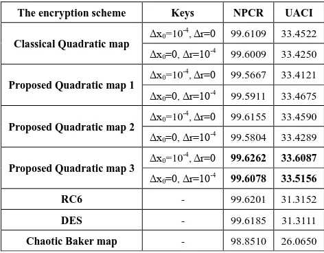
6.1.3. Sensitivity Analysis
In general, an encrypted image must be sensitive to the small changes in the original image and secret key. In order to avoid differential attack, a small change in the plain image or secret key should cause a significant change in the encrypted image. Two parameters were used for differential analysis; Net Pixel Change Rate (NPCR) and Unified Average Changing Intensity (UACI) [28]. NPCR measures the number of pixels change rate of encrypted image while one pixel of the original image is changed. UACI measures the average intensity of the differences between those two images. The NPCR and UACI of two encrypted images are defined in Eqs. (15), (16) respectively. C1 and C2 are two encrypted images, whose corresponding plain images have only one pixel change.
, ( , )
100%
i jD i j
NPCR
W H
(15)
1 2
,
( , ) ( , ) 1
100% 255
i j
C i j C i j UACI
W H
(16)where D(i,j) represents the difference between C1(i,j) and C2(i,j). If C1(i,j)= C2(i,j) then D(i,j)=0, otherwise D(i,j)=1. We can use these two parameters to measure the key sensitivity as follows.
(a) Key Sensitivity
We obtained the NPCR and UACI of the encrypted
Cameraman image under the change of the value of x0 and r,
on which the secret key depends. We used x0=0.02 and r= 2
as the first set of key, and then changed it. Table (4) shows the values of NPCR and UACI between encrypted images with keys (x0, r) and another slightly different key (Δx0, Δr).
Our results show that for all encryption algorithms with classical and proposed Quadratic maps, more than 99% of the pixels in the encrypted image change their gray values,
when the key is just changed by 10-4. The encryption
Table (4). NPCR and UACI between encrypted Cameraman images
UACI NPCR
Keys The encryption scheme
33.4522 99.6109
Δx0=10-4, Δr=0
Classical Quadratic map
33.4250 99.6009
Δx0=0, Δr=10-4
33.4121 99.5667
Δx0=10-4, Δr=0
Proposed Quadratic map 1
33.4675 99.5911
Δx0=0, Δr=10-4
33.4590 99.6155
Δx0=10-4, Δr=0
Proposed Quadratic map 2
33.4289 99.5804
Δx0=0, Δr=10-4
33.6087 99.6262
Δx0=10-4, Δr=0
Proposed Quadratic map 3
33.5156 99.6078
Δx0=0, Δr=10-4
31.3152 99.6201
-
RC6
31.3111 99.6185
-
DES
26.0650 98.8510
-
Chaotic Baker map
6.2. Processing Time
The processing time is the time required to encrypt and decrypt an image. The smaller the processing time, the better is the encryption efficiency. The proposed scheme uses only one round for diffusion process, and so this reduces the encryption/decryption time, and hence the scheme is practicable in real time applications. All the calculations are performed using MATLAB R2007a software under windows XP operating system, processor core 2 duo, 1.6 GHz and 2G RAM. For the 256 gray level Cameraman, Mandrill, and Lena images, the processing time is listed in Table (3). It is clear that the processing time of the proposed scheme is within 75 seconds, which is smaller than the processing time of RC6, and DES. Chaotic Baker map has the smallest processing time, because it is just a permutation map.
7. Conclusions
In this paper, new Quadratic chaotic maps with better chaotic properties have been proposed. These maps increase the available chaotic range of parameter r to infinity, and hence are more robust against attacks compared to the limited value of parameter r in the classical Quadratic map. The MLE in the proposed Quadratic maps is increased compared to the classical Quadratic map up to 3.4709, while it was 0.6720 in the classical Quadratic map. Therefore, the proposed Quadratic maps are more effective than the classical Quadratic map in the encryption process and more sensitive to the initial conditions. An encryption scheme of permutation and diffusion combining two chaotic maps has been presented and investigated. In the permutation process, we sort chaotic sequences of the Chepyshev map to shuffle the image. This procedure avoids the cycle of chaotic numbers in the generation of the permutation key. In the diffusion process, the permuted image is then encrypted by the key related to the plain image algorithm using the proposed Quadratic maps. In this encryption scheme, the key depends on both the initial key and the original image. So it
can survive known plain text attack. This algorithm uses a single round of diffusion, and hence it has low computational complexity. The proposed encryption scheme effectively resists the brute-force attack due to its very large key space. Furthermore, security, statistical, and sensitivity analysis has been carried out demonstrating high security and robustness of the proposed scheme. This proposed scheme is suitable for real-time image encryption applications due to its small processing time compared to the other encryption schemes. A comparative study have been presented between the proposed scheme, RC6, DES and chaotic Baker map. The results of this comparison show that the proposed scheme using the proposed Quadratic maps has a superior performance.
REFERENCES
[1] E B William, (2000), Data Encryption Standard, in NIST's anthology, A Century of Excellence in Measurements Standards and Technology: A Chronicle of Selected NBS/NIST Publications.
[2] FIPS PUB 197, (2001), Advanced Encryption Standard (AES), National Institute of Standards and Technology, U.S. Department of Commerce.
[3] C.E. Shannon, Communication Theory of Secrecy Systems, Bell System Technical Journal, vol. 28, No. 4, pp. 656-715, October 1949.
[4] Li, T.Y., Yorke, J.A. Period three implies chaos. The American Mathematical Monthly 82, 985{992 (1975). [5] Matthews, R. Cryptologia 1989, XIII, 29–42.
[6] Habutsu, T.; Nishio, Y.; Sasase, I.; Mori, S., Advancesincryptology-Eurocrypt’91, Lecture notes in computers cience 0547, Pp.127-140, Spinger-Verlag, Berlin, 1991.
[7] Fridrich, J. Int. J. Bifurcation and Chaos 1998, 8, 1259–1284. [8] Baptista, M. S. Phys. Lett. A 1998, 240, 50–54.
[9] Alexander N. Pisarchik, Massimiliano Zanin, Chaotic map cryptography and security In: Encryption: Methods, Software and Security Editor: Editor Name, pp. 1-28, 2010 Nova Science Publishers, Inc.
[10] Kelber, K.; Schwarz, W. NOLTA 2005, Bruges.
[11] http://math.arizona.edu/~urareports/041/Headington.Kenny/ Final_Report/quadraticmap.pdf
[12] S Li, (2007), Analyses and new designs of digital chaotic ciphers, Ph.D. dissertation, information and communications engineering, Xi’an Jiaotong Univeristy, China.
[13] M. T. Rosenstein, J. J. Collins, and C. J. de Luca, (1993), A practical method for calculating largest Lyapunov exponents from small data sets, Physical D: Nonlinear Phenomena, vol. 65, no. 1-2, pp.117–134.
Communications 275 (2), 324-329.
[15] Z-L. Zhu, W. Zhang, K-W Wong, H. Yu, (2011), A chaos-based symmetric image encryption scheme using bit-level permutation, Information Sciences 181 1171-1186. [16] C. Li, S. Li, K.-T. Lo, (2011), Breaking a modified
substitution-diffusion image cipher based on chaotic standard and logistic maps, Communications in Nonlinear Science and Numerical Simulation 16 (2) 837-843.
[17] K. Gupta, S. Silakari, (2011), New approach for fast color image encryption using chaotic map, Journal of Information Security 2 139-150.
[18] Fernando Jorge S. Moreira, (1992), Chaotic dynamics of quadratic maps, Master’s thesis, University of Porto. [19] V. Lynnyk, (2010), Chaos-Based Communication Systems.
Ph.D. thesis, Czech Technical University, Faculty of Electrical Engineering Department of Control Engineering, Prague.
[20] M. T. Rosenstein, J. J. Collins, and C. J. de Luca, (1993), A practical method for calculating largest Lyapunov exponents from small data sets, Physica D: Nonlinear Phenomena, 65, (1-2) 117–134.
[21] H. Kantz, (1994), A robust method to estimate the maximal
Lyapunov exponent of a time series, Physics Letters A, 185, (1) 77–87.
[22] Geisel, T., Fairen, V., (1984), Statistical properties of chaos in Chebyshev maps, Phys. Lett. A, 105, (6) 263–266.
[23] R Noha, HA HossamEldin, EE Said, and EA Fathi, (2015), Hybrid ciphering system of image based on fractional Fourier transform and two chaotic maps , International Journal of Computer Applications (0975 – 8887), 119 (11) 12–17. [24] J. Fridrich, Symmetric Ciphers Based on Two-Dimensional
Chaotic Maps, Int. J. Bifurcation and Chaos, Vol. 8, No. 6, pp. 1259–1284, 1998.
[25] http://in.mathworks.com/help/images/ref/corr2.html. [26] C Kevin, B Karen, (2003), An evaluation of image based
steganography methods, International Journal of Digital Evidence, volume no. 2, Issue 2.
[27] Chong Fu, Junjie Chen, Hao Zou, Weihong Meng, Yongfeng Zhan, and Yawe, (2012), A chaos based digital image encryption scheme with an improved diffusion strategy, Optics Express, volume no. 20.