www.geosci-instrum-method-data-syst.net/3/143/2014/ doi:10.5194/gi-3-143-2014
© Author(s) 2014. CC Attribution 3.0 License.
In-flight calibration of double-probe electric field
measurements on Cluster
Y. V. Khotyaintsev1, P.-A. Lindqvist2, C. M. Cully1,*, A. I. Eriksson1, and M. André1
1Swedish Institute of Space Physics, Uppsala, Sweden 2Royal Institute of Technology, Stockholm, Sweden
*now at: Department of Physics and Astronomy, University of Calgary, Calgary, Canada Correspondence to: Y. V. Khotyaintsev ([email protected])
Received: 19 August 2013 – Published in Geosci. Instrum. Method. Data Syst. Discuss.: 31 January 2014 Revised: 3 July 2014 – Accepted: 4 August 2014 – Published: 27 August 2014
Abstract. Double-probe electric field instrument with long wire booms is one of the most popular techniques for in situ measurement of electric fields in plasmas on spinning space-craft platforms, which have been employed on a large num-ber of space missions. Here we present an overview of the calibration procedure used for the Electric Field and Wave (EFW) instrument on Cluster, which involves spin fits of the data and correction of several offsets. We also describe the procedure for the offset determination and present results for the long-term evolution of the offsets.
1 Introduction
Double-probe electric field experiments have been flown on a number of spacecraft (see review by Pedersen et al., 1998) including Cluster (Gustafsson et al., 1997, 2001), and cali-bration of the direct-current (DC) electric field has always been a challenging and time-consuming task. Main reasons for this are strong influence of the ambient plasma and the spacecraft itself on the measurements. Other techniques to measure electric fields at low time resolution as electron drift instruments and ion spectrometers, such as Electron Drift In-strument (EDI) (Paschmann et al., 1997, 2001) and Cluster Ion Spectrometry (CIS) (Rème et al., 2001) on Cluster, are immune to some of the problems affecting the double-probe measurements, but have their own limitations. With the Clus-ter Active Archive a semi-automatic approach to in-flight calibration of the DC electric field data has been developed (Khotyaintsev et al., 2010), and the purpose of this paper is
to describe the main elements of this calibration procedure under nominal operations.
An example of a clear deviation from nominal perfor-mance is the non-geophysical electric field detected by Elec-tric Field and Wave experiment (EFW) due to the wake be-hind the spacecraft caused by cool (eV) outflowing iono-spheric ions drifting at supersonic velocities (Eriksson et al., 2006). Such ions are common in the magnetospheric tail lobes. Careful investigation of this “problem” has resulted in a new method to detect positive low-energy ions, other-wise invisible to detectors on a sunlit spacecraft positively charged to several volts (Engwall et al., 2006, 2009a, b; An-dré and Cully, 2012). However, it is not possible to recover the ambient geophysical electric field in such cases.
2 Short instrument description
144 Y. V. Khotyaintsev et al.: DC electric field calibration
Discussion
P
a
per
|
Discu
ssion
P
a
per
|
Discussion
P
a
per
|
Discussion
P
a
per
|
2,9m 62m
88m 1
2 3
4
Figure 1.Cluster EFW double-probe electric field instrument.
16
Figure 1. Cluster EFW double-probe electric field instrument.
a cut-off frequency of 10 Hz. A detailed description of the EFW instrument can be found in Gustafsson et al. (1997, 2001).
3 Calibration procedure
The goal of the calibration procedure is to obtain geophysi-cal DC electric field in the spacecraft spin plane in a despun reference frame. On Cluster we used the ISR2 (Inverted Spin Reference) system, also known as DSI (Despun System In-verted). Thex andy axes are in the spin plane, withx axis pointing as near sunward as possible andyaxis perpendicu-lar to the sunward direction, positive towards dusk. Thezaxis is along the (negative) spacecraft spin axis, towards the north ecliptic. The coordinate system is called “inverted” because the actual spin axis of Cluster is pointing towards the south ecliptic. The ISR2 system thus is identical to Geocentric So-lar Ecliptic system (GSE) if the satellite spin axis angle to ecliptic north is zero, and is a good approximation to GSE for the usual case of this angle being a few degrees.
3.1 Raw data
The raw data available from EFW under normal circum-stances are the two orthogonal electric field components in the spinning frame (E12 andE34) sampled at 25 or 450 Hz,
as well as potentials of the individual probes (P1,P2,P3and
P4) sampled at 5 Hz. In case of probe 1 failure (for dates of
permanent failures on C1, C2 and C3, see Lindqvist et al., 2013), instead of E12 we use E32. An example of raw data is shown in Fig. 2.
As the first stage of calibration, it is necessary to perform initial cleaning of the data at which we remove intervals with bad data due to issues with electronics, probe satura-tions due to low plasma density (often occurring in in the magnetospheric lobes), and saturations due to non-optimal
Discussion
P
a
per
|
Discu
ssion
P
a
per
|
Discussion
P
a
per
|
Discussion
P
a
per
|
14 1
2
Figure 2. Raw data of the electric field, E12, E34 (upper panel) and of the probe-to-spacecraft
3
potential P1, P2, P3, P4, (bottom panel) measured by Cluster 1.
4 5
Figure 2.Raw data of the electric field,E12,E34(upper panel) and of the probe-to-spacecraft
potentialP1,P2,P3,P4, (bottom panel) measured by Cluster 1. 17
Figure 2. Raw data of the electric field,E12,E34(upper panel) and of the probe-to-spacecraft potentialP1,P2,P3,P4(bottom panel) measured by Cluster 1.
bias current settings occurring in dense plasmas such as mag-netosheath and plasmasphere (Khotyaintsev et al., 2010). If the spacecraft is in the solar wind, we apply a correction for the wakes usually present in the raw data (Eriksson et al., 2007).
3.2 Spin fits
After initial cleaning of the data, a spin fitting procedure is performed; the output of this procedure provides basic pa-rameters that are used later in the calibration procedure. In the presence of a constant ambient electric field, the raw data signal (probe potential difference) is a sine wave (see Fig. 2, upper panel) where the amplitude and phase give the electric field magnitude and direction. A least-squares fit to the raw data of the form
y=A+Bsin(ωt )+Ccos(ωt )+Dsin(2ωt )
+Ecos(2ωt )+. . . (1)
is done once every 4 s (2π/ω≈4 s is approximately the spacecraft spin period) and the fit is applied to 4 s long time intervals.
Y. V. Khotyaintsev et al.: DC electric field calibration 145 3.3 Offsets
The sine and cosine terms,BandC, after correction for ISR2 offsets provide the 4 s (spin) resolution electric field in ISR2:
Ex4s=α (B−1Ex) , (2)
Ey4s=α C−1Ey, (3)
whereαis the amplitude correction factor due to the ambient electric field being “short-circuited” by the presence of the spacecraft and wire booms (see Sect. 4.1). And1Ex
(sun-ward offset) and 1Ey (duskward offset) are the ISR2 off-sets, which represent the difference between the measured
and geophysical electric fields in the despun frame and are discussed in detail later.
As the spin fitting procedure would typically yield dif-ferent values for the electric field from the two difdif-ferent probe pairs, it is useful to introduce an additional offset which describes the difference between the two measure-ments,1p12p34, which we call the delta offset:
1xp12p34=Ex4s(E12)−Ex4s(E34) , (4)
1yp12p34=Ey4s(E12)−Ey4s(E34) . (5)
The despun full-resolution electric field is obtained as follows:
Ex=Re [ε12]−1xp12p34+Re [ε34], (6)
Ey=Im [ε12]−1yp12p34+Im [ε34], (7)
where ε12=(E12−1raw 12) eiφ12, ε34=(E34−1raw 34)
eiφ34, andφ12=φ34+π/2 is the spin phase of probe 1 with
respect to the sun; raw data DC offset,1raw= hAi, is based
on parameterAof the fit (Eq. 1). Ideally, the DC level of the raw data should be zero. However, small differences between the probe surfaces and in the electronics create a DC offset in the raw data. If not corrected, it shows up as a signal at the spin frequency in the despun electric field.
It must be noted that asymmetries due to the direction to the sun have the dominant contribution to the offsets, so that the following inequalities are typically satisfied:
1Ex 1Ey, (8)
1xp12p34 1yp12p34. (9)
4 Results
In this section we summarize the main results concerning the various offsets defined above. Raw data DC offset and delta offsets are obtained from spin fits, while the amplitude cor-rection factor and ISR2 offsets are obtained based on inter-spacecraft calibration as well as cross-calibration with CIS (Rème et al., 2001) and EDI (Paschmann et al., 1997, 2001).
P
a
per
|
Discu
ssion
P
a
per
|
Discussion
P
a
per
|
Discussion
P
a
per
|
09−Nov−2002 29−Dec−2002 17−Feb−2003 08−Apr−2003 28−May−2003 1
1.05 1.1 1.15 1.2 1.25 1.3 1.35
∆
amp
C1 C2 C3 C4
Figure 3.Amplitude correction factor for the electric field measured by EFW on cluster 1–4
during a solar wind season from November 2002 to June 2003.
18
Figure 3. Amplitude correction factor for the electric field measured by EFW on Cluster 1–4 during a solar wind season from Novem-ber 2002 to June 2003.
4.1 Amplitude factors
Amplitude factors are needed since the electric field is par-tially “short circuited” by the spacecraft potential, which is also the potential of the wire booms, extending out to a large distance from the spacecraft (Cully et al., 2007).
We have used the ISR2ycomponents of the electric field to determine the amplitude correction factor. This component ofEis generally free from offsets, and thus by comparingEy
from EFW and CIS-HIA we are able to deduce the ampli-tude correction factor. Results of such computations for the spring season of 2002 are shown in Fig. 3. Every point in the plot corresponds to one orbit of data. One should mention that variations seen in the data are not caused by changes in the factor, but rather by “bad data” and insufficient data coverage.
On the basis of simulations and comparisons with other Cluster instruments, it has been determined that the mea-sured electric field magnitude needs to be multiplied by a factor ofα=1.1. We use this constant value through the en-tire mission. This value is consistent with valued obtained from simulations of the spacecraft–plasma interaction (Cully et al., 2007).
4.2 Raw data DC offset
The raw data DC offset,1raw, from the both probe pairs is
used to calculate the full-resolution E-field. It is applied to E12 andE34 prior to despinning. Variations in the electric
field will result in small changes toAcomputed from spin fits for different 4 s intervals. So if1raw depended only on
the electronics, one could compute a long-term average of Aand use it as1raw. But we find that Aalso depends on
146 DiscussionY. V. Khotyaintsev et al.: DC electric field calibration
P
a
per
|
Discu
ssion
P
a
per
|
Discussion
P
a
per
|
Discussion
P
a
per
|
−60 −50 −40 −30 −20 −10 0 −0.1
0 0.1 0.2 0.3 0.4 0.5 0.6
ScPot [−V]
Dadc [mV/m]
C1 p34 2002−10−18T00:00:00Z −− 30 hours
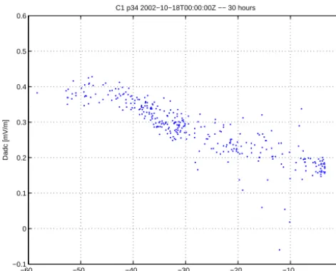
Figure 4.Dependence of the raw data DC offset,∆raw, computed from the spin fits on the
spacecraft potential showing that the offset decreases when the potential is close to zero (char-acteristic of dense plasmas).
19
Figure 4. Dependence of the raw data DC offset,1raw, computed from the spin fits on the spacecraft potential showing that the offset decreases when the potential is close to zero (characteristic of dense plasmas).
Therefore we want a smoothened value and at the same time to track changes in the plasma environment. That is why the DC offset is smoothed, 1raw= hAi, using a weighted
aver-age over seven spins using weights [0.07, 0.15, 0.18, 0.2, 0.18, 0.15, 0.07]. This approach was selected based on an empirical basis after testing several different lengths of the averaging interval.
4.3 ISR2 offsets
Our main assumption in the study of ISR2 offsets is that the offsets depend on the instrument configuration, spacecraft at-titude and that the dependence on surrounding plasma param-eters is weak, i.e., being in the same kind of plasma environ-ment (for example plasma sheet) and having the same instru-ment settings and probe properties for two different time in-tervals, and the difference between ISR2 offsets for the two intervals must be within the uncertainty of the offset deter-mination (fraction of mV m−1). As the offsets still depend on the plasma environment, we decided to split the data set into two groups – “solar wind/magnetosheath” and “magne-tosphere” – which correspond to two situations with “cold and dense” and “hot and rarefied” plasmas. To split every orbit into these two groups, we have used the Shue magne-topause model (Shue et al., 1997) with realistic solar wind parameters measured by the ACE spacecraft. For each of the groups we statistically determine offsets over a period of sev-eral weeks to sevsev-eral months in order to account for changes in the instrument setting, spacecraft attitude, solar UV flux, etc. Then, based on the position along the orbit, observed value of the spacecraft potential and manual inspection, we
determine which of the two offsets is to be applied at each point.
4.3.1 ISR2 offsets in the solar wind and magnetosheath For the solar wind/magnetosheath intervals, we first perform the inter-spacecraft calibration under assumption that all the spacecraft observe the same large-scale electric field, which is the case in the solar wind. As a result for each interval (from outbound magnetopause crossing to the inbound, typ-ically several hours long), we get relative offset between the spacecraft, which are the differences inExandEybetween
the different spacecraft averaged over the entire interval. Fig-ure 5 shows an example of such an interval, and the two upper panels showExandEyfrom all four spacecraft.
Then by using CIS-HIA from C1 and/or C3 as reference data, we find the ISR2 offsets for EFW for each of the space-craft. We get one value for offsets per orbit. The procedure can be controlled visually by using a type of plot presented in Fig. 5. The two upper panels show all the available EFW and CIS-HIA data (ExandEy in ISR2). Then we construct
the reference E-field from CIS-HIA by averaging data from the spacecraft where CIS-HIA data are available. Such av-eraging is possible as the difference between the spacecraft in the solar wind/magnetosheath is typically small. Then we compute the difference between the EFWEx on all
space-craft and the reference E-field; this difference is plotted in the third panel. Average of the difference over the entire in-terval gives the local IRS2 offset. This offset is then applied to the EFW on different spacecraft. The resulted corrected and reference E-fields are plotted in the two bottom panels.
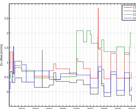
Evolution of ISR2 offsets in the solar wind and magne-tosheath during mission lifetime is shown in Fig. 6. One can see that the offsets are rather steady and slowly decreas-ing with approach of the solar minimum (∼2009). The only striking feature is the sudden increase of the offset in C3 in 2005. This change is not yet understood.
4.3.2 ISR2 offsets in the magnetosphere
The problem of determining the offsets in the magnetosphere is significantly more complicated in comparison to the solar wind/magnetosheath. Data from the other instruments, which could have been used as a reference, are of very low quality in large areas of the magnetosphere due to low counts (the CIS instrument) or low magnetic fields (the EDI instrument). Also the EFW data are subject to frequent problems, such as electrostatic wakes, and the data affected by wakes need to be excluded from the data set used to determine the offsets.
In the ISR2 offset determination procedure, we decided not to use any reference data, but rather to use a condition of zero electric fieldhExi =0, as most of the time the
Y. V. Khotyaintsev et al.: DC electric field calibration 147
Discussion
P
a
per
|
Discu
ssion
P
a
per
|
Discussion
P
a
per
|
Discussion
P
a
per
|
−5
0 5
Ex [mV/m]
SH/SW 2001−02−21T12:00:00.000Z −− 2001−02−23T09:00:00.000Z EFW (−−), CIS HIA (+)
−5
0 5
Ey [mV/m]
0
0.5 1 1.5 2
dEx [mV/m]
−20
−15 −10 −5 0
Sc pot [
−
V]
235 reference points (87% data coverage)
−4
−2 0 2 4
dEx1=0.57, dEx2=1.04, dEx3=0.45, dEx4=0.15
Ex [mV/m]
12:00 16:00 20:00 00:00 04:00 08:00 12:00 16:00 20:00 00:00 04:00 08:00 −4
−2 0 2 4
21−Feb−2001
Ey [mV/m]
Figure
5.
Inter-spacecraft
calibration
and
cross-calibration
with
CIS
in
the
solar
wind/magnetosheath. Panels from top to bottom show
E
x
and
E
y
measured by EFW (solid
lines) on the 4 spacecraft and by CIS-HIA (
+
) on C1 and C3, di
ff
erence in
E
x
between CIS and
EFW (median value from all spacecraft), the spacecraft potential, and the two bottom panels
show the same data as on the top, but with the o
ff
sets applied to the EFW data. Data from the
four Cluster spacecraft shown by black (C1), red (C2), green (C3) and blue (C4).
Figure 5. Inter-spacecraft calibration and cross-calibration with CIS in the solar wind/magnetosheath. Panels from top to bottom showEx andEymeasured by EFW (solid lines) on the four spacecraft and by CIS-HIA (+) on C1 and C3, difference inExbetween CIS and EFW (median value from all spacecraft), the spacecraft potential, and the two bottom panels show the same data as on the top, but with the offsets applied to the EFW data. Data from the four Cluster spacecraft shown by black (C1), red (C2), green (C3) and blue (C4).
estimate for the ISR2Ex offset. The resulting offsets were
verified against the CIS data for a large number of cases, and in particular in the central plasma sheet the agreement is very good.
Results for Cluster 4 for years 2002–2005 are summarized in Fig. 7. One can see that there is a prominent peak around
148 Y. V. Khotyaintsev et al.: DC electric field calibration Discussion P a per | Discu ssion P a per | Discussion P a per | Discussion P a per |
2002 2003 2004 2005 2006 2007 2008 2009 2010 0 0.5 1 1.5 2 2.5
Ex offset [mV/m]
Time [year]
C1 C2 C3 C4
Figure 6.Long-term evolution of the ISR2Ex(sunward) offset in the Solar wind/magnetosheath
from 2001 to 2009.
21
Figure 6. Long-term evolution of the ISR2Ex(sunward) offset in the solar wind/magnetosheath from 2001 to 2009.
Discussion P a per | Discu ssion P a per | Discussion P a per | Discussion P a per |
0 0.5 1 1.5 2 2.5 3 3.5 0 0.02 0.04 0.06 0.08 0.1 0.12 0.14 0.16 0.18
. 1.29 mV/m
. 1.43 mV/m . 1.15 mV/m
. 1.37 mV/m
∆ Ex [mV/m]
Offset PDF
C4
2002 1.29 mV/m 2003 1.43 mV/m 2004 1.15 mV/m 2005 1.37 mV/m
Figure 7.Probability distribution function of ISR2Ex(sunward) offset for Cluster 4 in the
mag-netosphere for 2002–2005.
22
Figure 7. Probability distribution function of ISR2Ex (sunward) offset for Cluster 4 in the magnetosphere for 2002–2005.
Evolution of ISR2 offsets in the magnetosphere during mission lifetime is shown in Fig. 8. The offsets are steady and slowly decreasing with approach of the solar minimum. 4.4 Delta offset
Given the two identical probe pairs, we are able to estimate the electric field at the timescale of the spacecraft spin from each of them, and in principle these estimates should be iden-tical. In reality the probes are not identical, and the estimates of the electric fields differ. Such a difference is described by the delta offset. Figure 9 shows how the delta offsets change over time. The curves show the raw data, i.e., the differ-ence between the electric fields computed from the two probe pairs averaged over 1.5 h long intervals of data. One can see
Discussion P a per | Discu ssion P a per | Discussion P a per | Discussion P a per |
2002 2003 2004 2005 2006 2007 2008 2009 2010 0.5
1 1.5 2 2.5
Ex offset [mV/m]
Time [year]
C1 C2 C3 C4
Figure 8.Long-term evolution of the ISR2 offsets in the magnetosphere from 2001 to 2009.
23
Figure 8. Long-term evolution of the ISR2 offsets in the magneto-sphere from 2001 to 2009.
that the offset varies very slowly, at a typical timescale of sev-eral months, and with some sudden jumps typically related to spacecraft manoeuvres. Therefore for the calibration pur-poses we use a smoothened version of the offset, i.e., median over approximately two orbits. This approach allows us to get rid of the outliers, which can be caused by intervals with non-optimal instrument performance or strong geophysical electric fields.
Figure 10 shows the long-term evolution of the delta off-sets for all four spacecraft. Variations in the offset are caused by a number of factors. First is the solar cycle. One can see that the offset is rather small and steady in the beginning of the mission and starts to grow with approach of the solar min-imum, reaching its maximum in spring 2006. This behavior is caused by non-optimal bias current settings, and the sit-uation became significantly improved by lowering the bias current in June 2006. The second cause is the probe failures, which forced usage of P32 (shorter base and asymmetric with respect to the spacecraft) instead of P12 (see Fig. 1).
5 Discussion and conclusions
Discussion
P
a
per
|
Discu
ssion
P
a
per
|
Discussion
P
a
per
|
Discussion
P
a
per
|
−1 −0.5 0 0.5 1
E C1 [mV/m]
−1 −0.5 0 0.5 1
E C2 [mV/m]
−1 −0.5 0 0.5 1
E C3 [mV/m]
2002 2003 2004 2005 −1.5
−1 −0.5 0 0.5 1
E C4 [mV/m]
XY
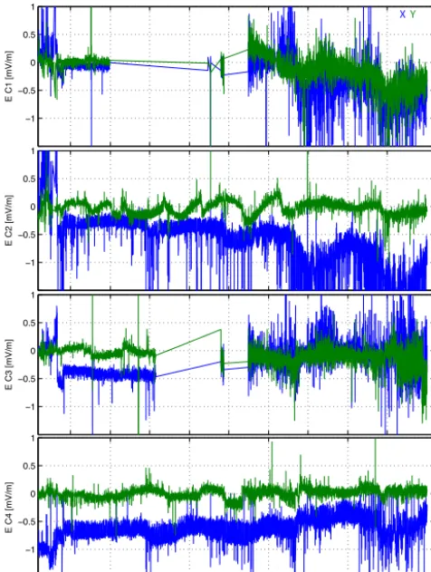
Figure 9.Evolution of the “raw” Delta offsets on Cluster 1–4 from 2001 to 2005. The blue and
green lines showX andY components of the difference between the electric fields computed from the different probe pairs, i.e. the “raw” delta offsets. In order to get rid of the outliers (spikes), we compute the median of this difference, which is then used as the delta offset applied to data during the calibration process.
24
Figure 9. Evolution of the “raw” delta offsets on Cluster 1–4 from 2001 to 2005. The blue and green lines showXandY components of the difference between the electric fields computed from the dif-ferent probe pairs, i.e., the “raw” delta offsets. In order to get rid of the outliers (spikes), we compute the median of this difference, which is then used as the delta offset applied to data during the cal-ibration process.
that most of the offsets have a rather slow variation with time on time–space timescales of weeks and month.
Both the amplitude factor (boom shortening) and the sun-ward offset depend on the Debye length and the spacecraft potential. For the Debye length shorter than the probe-to-puck distance (1.5 m for EFW), there is no boom shortening (i.e., amplitude factor=1); for the longer Debye length the effective boom length is shorter than the physical length, and such a shortening in some way depends on the spacecraft po-tential. We were unable to establish an empirical relation of the shortening factor with the spacecraft potential for EFW and used a constant amplitude factor for the CAA calibration as the measurement is performed in the long Debye length regime most of the time. We note that even determination of the Debye length on a routine basis is a challenging task for Cluster, due to high uncertainties and insufficient time reso-lution of the electron data.
Factors determining the sunward offset are much less un-derstood. Simulations by Cully et al. (2007) suggested that
Figure 10. Long-term evolution of delta offsets from 2001 to 2009 for C1 (black), C2 (red), C3 (green) and C4 (blue).
the offset appears due to an asymmetric photoelectron cloud around the spacecraft. However, analyzing changes in the sunward offset for EFW we found that the offset may be strongly driven by other factors, not only for the photoelec-tron cloud asymmetry. For example the offset in the solar wind depends on the solar wind speed in such a way that it decreases with an increase of the wind speed, and for suf-ficiently fast solar wind the offset turns into anti-sunward. Qualitative and quantitative understanding of the dependence of the amplitude factor and sunward offset on the surround-ing plasma remains an open question, which will be ad-dressed in the future by advanced numerical simulations and possibly by empirical comparison of the electric field mea-surements by the double probes to EDI and particle instru-ments on Magnetospheric Multiscale (MMS) Mission.
Using particle measurements to determine time-dependent offsets and to correct the EFW data on a routine basis showed to be practically impossible for Cluster, as such a correction would typically introduce a large random error into the elec-tric field measurement. However, we do no exclude a possi-bility for such a correction for case studies where one has full control of the quality of the reference data used to determine the offsets. Our choice of the calibration procedure for the CAA which is outlined in this paper is to rely solely on the EFW data for high-time-resolution calibrations, and then to use statistical offsets determined by averaging large amounts of data, and among others by comparison with the particle measurements.
150 Y. V. Khotyaintsev et al.: DC electric field calibration the plasma environment in a very similar way, and the effect
of these changes on offsets is not too drastic. Developing a procedure that would produce reliable results also for such cases during routine data production remains a challenging task.
As a concluding remark, we note that the described cali-bration procedure applies to data acquired when the instru-ment operates close its optimal regime, so that one can re-construct the ambient electric field present in the plasma by applying relatively small corrections. However, a major ef-fort during the CAA production goes into detection of strong deviations from the nominal operations (Khotyaintsev et al., 2010), which can be caused by both changes of the plasma environment surrounding the spacecraft and non-optimal in-strument settings.
Acknowledgements. The authors thank Andris Vaivads and other
colleagues for continuing support and discussion around the coffee breaks.
Edited by: H. Laakso
References
André, M. and Cully, C. M.: Low-energy ions: a previously hid-den solar system particle population, Geophys. Res. Lett., 39, L03101, doi:10.1029/2011GL050242, 2012.
Cully, C. M., Ergun, R. E., and Eriksson, A. I.: Electrostatic struc-ture around spacecraft in tenuous plasmas, J. Geophys. Res., 112, A09211, doi:10.1029/2007JA012269, 2007.
Engwall, E., Eriksson, A. I., André, M., Dandouras, I., Paschmann, G., Quinn, J., and Torkar, K.: Low-energy (or-der 10 eV) ion flow in the magnetotail lobes inferred from spacecraft wake observations, Geophys. Res. Lett., 33, L06110, doi:10.1029/2005GL025179, 2006.
Engwall, E., Eriksson, A. I., Cully, C. M., André, M., Torbert, R., and Vaith, H.: Earth’s ionospheric outflow dominated by hidden cold plasma, Nat. Geosci., 2, 24–27, 2009a.
Engwall, E., Eriksson, A. I., Cully, C. M., André, M., Puhl-Quinn, P. A., Vaith, H., and Torbert, R.: Survey of cold ionospheric outflows in the magnetotail, Ann. Geophys., 27, 3185–3201, doi:10.5194/angeo-27-3185-2009, 2009b.
Eriksson, A. I., André, M., Klecker, B., Laakso, H., Lindqvist, P.-A., Mozer, F., Paschmann, G., Pedersen, A., Quinn, J., Torbert, R., Torkar, K., and Vaith, H.: Electric field measurements on Cluster: comparing the double-probe and electron drift techniques, Ann. Geophys., 24, 275–289, doi:10.5194/angeo-24-275-2006, 2006. Eriksson, A. I., Khotyaintsev, Y., and Lindqvist, P.-A.: Spacecraft
wakes in the solar wind, in: Proceedings of the 10th Space-craft Charging Technology Conference (SCTC-10), available at: http://www.space.irfu.se/aie/publ/Eriksson2007b.pdf (last ac-cess: 30 January 2014), 2007.
Gustafsson, G., Boström, R., Holback, B., Holmgren, G., Lund-gren, A., Stasiewicz, K., Åhlén, L., Mozer, F. S., Pankow, D., Harvey, P., Berg, P., Ulrich, R., Pedersen, A., Schmidt, R., Butler, A., Fransen, A. W. C., Klinge, D., Thomsen, M., Fälthammar, C.-G., Lindqvist, P.-A., Christenson, S., Holtet, J.,
Lybekk, B., Sten, T. A., Tanskanen, P., Lappalainen, K., and Wygant, J.: The Electric Field and Wave Experiment for the Clus-ter Mission, Space Sci. Rev., 79, 137–156, 1997.
Gustafsson, G., André, M., Carozzi, T., Eriksson, A. I., Fältham-mar, C.-G., Grard, R., Holmgren, G., Holtet, J. A., Ivchenko, N., Karlsson, T., Khotyaintsev, Y., Klimov, S., Laakso, H., Lindqvist, P.-A., Lybekk, B., Marklund, G., Mozer, F., Mursula, K., Peder-sen, A., Popielawska, B., Savin, S., Stasiewicz, K., Tanskanen, P., Vaivads, A., and Wahlund, J.-E.: First results of electric field and density observations by Cluster EFW based on initial months of operation, Ann. Geophys., 19, 1219–1240, doi:10.5194/angeo-19-1219-2001, 2001.
Khotyaintsev, Y., Lindqvist, P.-A., Eriksson, A. I., and André, M.: The EFW Data in the CAA, the Cluster Active Archive, Study-ing the Earth’s Space Plasma Environment, in: Astrophysics and Space Science Proceedings, edited by: Laakso, H., Tay-lor, M. G. T. T., and Escoubet, C. P., Springer, Berlin, 97–108, 2010.
Lindqvist, P.-A., Cully, C. M., and Khotyaintsev, Y.: User Guide to the EFW measurements in the Cluster Active Archive (CAA), available at: http://caa.estec.esa.int/caa/ug_cr_icd.xml (last ac-cess: 30 January 2014), 2013.
Paschmann, G., Melzner, F., Frenzel, R., Vaith, H., Parigger, P., Pagel, U., Bauer, O., Haerendel, G., Baumjohann, W., Sck-opke, N., Torbert, R., Briggs, B., Chan, J., Lynch, K., Morey, K., Quinn, J., Simpson, D., Young, C., McIlwain, C., Fillius, W., Kerr, S., Mahieu, R., and Whipple, E.: The electron drift instru-ment for cluster, Space Sci. Rev., 79, 233–269, 1997.
Paschmann, G., Quinn, J. M., Torbert, R. B., Vaith, H., McIlwain, C. E., Haerendel, G., Bauer, O. H., Bauer, T., Baumjohann, W., Fillius, W., Förster, M., Frey, S., Georgescu, E., Kerr, S. S., Kletzing, C. A., Matsui, H., Puhl-Quinn, P., and Whipple, E. C.: The Electron Drift Instrument on Cluster: overview of first results, Ann. Geophys., 19, 1273–1288, doi:10.5194/angeo-19-1273-2001, 2001.
Pedersen, A., Mozer, F., and Gustafsson, G.: Electric field mea-surements in a tenuous plasma with spherical double probes, in: Measurement Techniques in Space Plasmas – Fields: Geophysi-cal Monograph 103, edited by: Pfaff, R. F., Borovsky, J. E., and Young, D. T., published by the American Geophysical Union, Washington, D.C., USA, 1–12, 1998.
magnetosphere with the identical Cluster ion spectrometry (CIS) experiment, Ann. Geophys., 19, 1303–1354, doi:10.5194/angeo-19-1303-2001, 2001.