www.wind-energ-sci.net/2/115/2017/ doi:10.5194/wes-2-115-2017
© Author(s) 2017. CC Attribution 3.0 License.
Optimization of wind plant layouts using an
adjoint approach
Ryan N. King1,2, Katherine Dykes2, Peter Graf2, and Peter E. Hamlington1 1University of Colorado, Boulder, Colorado, USA
2National Renewable Energy Laboratory, Golden, Colorado, USA
Correspondence to:Ryan N. King ([email protected])
Received: 17 July 2016 – Discussion started: 31 August 2016
Revised: 6 December 2016 – Accepted: 6 January 2017 – Published: 10 March 2017
Abstract. Using adjoint optimization and three-dimensional steady-state Reynolds-averaged Navier–Stokes (RANS) simulations, we present a new gradient-based approach for optimally siting wind turbines within utility-scale wind plants. By solving the adjoint equations of the flow model, the gradients needed for optimization are found at a cost that is independent of the number of control variables, thereby permitting optimization of large wind plants with many turbine locations. Moreover, compared to the common approach of superimposing pre-scribed wake deficits onto linearized flow models, the computational efficiency of the adjoint approach allows the use of higher-fidelity RANS flow models which can capture nonlinear turbulent flow physics within a wind plant. The steady-state RANS flow model is implemented in the Python finite-element packageFEniCSand the derivation and solution of the discrete adjoint equations are automated within thedolfin-adjoint frame-work. Gradient-based optimization of wind turbine locations is demonstrated for idealized test cases that reveal new optimization heuristics such as rotational symmetry, local speedups, and nonlinear wake curvature effects. Layout optimization is also demonstrated on more complex wind rose shapes, including a full annual energy production (AEP) layout optimization over 36 inflow directions and 5 wind speed bins.
1 Introduction
Optimizing wind turbine locations within a wind plant is a uniquely challenging problem that combines turbulent flow control with practical engineering challenges concerning the economical development of renewable energy. The prob-lem is further complicated by the strong nonlinear coupling between turbine locations, power production, atmospheric boundary layer turbulence, and mechanical loads on turbine components. Wind plant optimization techniques used in in-dustry often rely on heuristic guidelines and simplified linear flow models that limit computational costs. However, these approaches neglect important turbulent flow physics and can result in the underperformance of wind plants relative to their pre-construction estimates. The reduced power output and increased uncertainty due to optimization with low-fidelity flow models ultimately increases the levelized cost of energy (LCOE) and associated project risk for investors.
provide optimized layouts with arbitrary topological com-plexity at relatively low computational cost, while at the same time more accurately capturing turbulent flow effects present in real wind plants.
This paper is organized as follows: background on wind plant flow modeling, layout optimization, and adjoint opti-mization techniques is provided in Sect. 2; a description of the methods used in WindSE for implementing the wind plant optimization problem, flow model, turbine represen-tation, numerics, and optimization algorithm is given in Sect. 3; a demonstration of the flow model capabilities and optimization results for idealized and real world test cases with increasingly complex wind roses, culminating in a full annual energy production (AEP) optimization, is presented in Sect. 4; and the paper is concluded with a discussion of the results and implications for wind plant design in Sect. 5.
2 Background
2.1 Wind plant flow modeling
Utility-scale wind plants in the United States typically in-volve tens to hundreds of turbines arranged in semi-regular arrays. The layout topology is generally an outcome of opti-mizing the power production or net capacity factor subject to competing influences from site constraints, the local wind re-source, and construction costs. These constraints include the patchwork of viable building areas formed by leases and set-backs due to environmental concerns or physical infrastruc-ture, terrain and soil characteristics like slope or vegetation, turbine manufacturer spacing requirements, and continuity requirements imposed by access roads and electrical connec-tions. This results in a complex design problem, with turbine layouts varying drastically between different geographic lo-cations and exhibiting complex topologies.
The AEP from a wind plant layout has traditionally been, and generally continues to be, assessed using reduced-order linear flow models. Such models estimate the relative wind speed across a site based on the linearized Navier–Stokes equations and treat terrain features as perturbations in bound-ary conditions. The underlying governing equations, intro-duced by Jackson and Hunt (1975) and implemented in packages such as MS3DJH/3R (Walmsley et al., 1986), are based on analytical perturbation solutions to flow over a low hill. This approach decomposes the terrain into sinusoidal hills and calculates relative speedup effects over each hill. Speedup effects from multiple hills are superimposed to ob-tain relative velocities over the entire site. The emphasis on relative velocities is motivated by the need to extrapolate from point measurements at meteorological towers to veloc-ity fields covering the entire plant.
A velocity deficit representing the turbine wake is then su-perimposed on the background wind resource at each turbine location. The PARK model developed by Jensen (1983) and the eddy viscosity model developed by Ainslie (1988) are
commonly used, and a comprehensive review of wake mod-eling can be found in Crespo et al. (1999). Such approaches decouple the wind flow calculation from the wake calculation and use wake models calibrated to a single turbine in iso-lation. As a result, the wake model approach neglects flow curvature, speed-up effects around turbines, and changes to wakes deep in a plant. This results in known inaccura-cies in complex terrain, ad hoc model adjustments for over-lapping wakes from multiple turbines, and systemic under-predictions of wake losses and over-under-predictions of power out-put (Barthelmie et al., 2009). Despite these limitations, linear flow models and prescribed wake models are commonly used in engineering practice because they are computationally in-expensive and reasonably accurate in simple terrain with few turbines.
Recently, higher-fidelity computational fluid dynamics (CFD) models have been increasingly applied to the study of wind plant performance. Several RANS models have been developed for simulating atmospheric flows in wind plants using actuator disk turbine representations, with a particular emphasis on modifiedk−closures (Cabezón et al., 2011; El Kasmi and Masson, 2008; van der Laan et al., 2015a, b). These approaches greatly improve upon linearized flow models and, given an appropriate model for the turbulent eddy viscosity, better capture turbulent transport effects in the shear layer at the edge of the wake. Large eddy simulation (LES) is also increasingly being applied to wind plant mod-eling (Calaf et al., 2010; Porté-Agel et al., 2011; Churchfield et al., 2012), as well as to some aspects of wind plant opti-mization. These simulations are vastly more expensive than RANS approaches, but resolve time-varying turbulent mo-tions up to the filter cutoff scale. This allows for better char-acterization of wake meandering and unsteady loads on tur-bines. Finally, wind plant modeling has also been improved through coupling to numerical weather prediction simula-tions (Fitch et al., 2012; Mirocha et al., 2014). Such simu-lations are able to incorporate synoptic-scale weather forc-ing and interactions between the surface, wind plant, and full atmospheric boundary layer.
2.2 Approaches to wind plant optimization
(Mar-den et al., 2013). An exhaustive review of wind plant opti-mization efforts has been compiled by Herbert-Acero et al. (2014) that surveys the wide variety of objective functions, flow models, and constraints that have been studied. Results from these prior optimizations are, however, heavily influ-enced by the use of analytical wake models which do not fully account for nonlinear and turbulent flow physics. Con-sequently, significant differences in optimal layouts are ex-pected when using higher-fidelity flow models.
Recently, higher-fidelity CFD flow models have been used in a limited range of wind plant optimization applications. The Technical University of Denmark has developed TOP-FARM (Larsen et al., 2011), which employs an improved wake model (the dynamic wake meandering model) as well as a parabolic Navier–Stokes solver. TOPFARM uses a hy-brid optimization approach that combines sequential linear programming (SLP) with gradient-free genetic algorithms. The genetic algorithm is used to find the neighborhood of the global optimum, and then the gradient-based SLP rithm completes the optimization. However, the genetic algo-rithm step penalizes large design spaces, limiting TOPFARM to relatively small wind plants. King et al. (2016) used ad-joints of a 2-D RANS flow model to optimize turbine lo-cations and observed that the 2-D nature of the flow solver resulted in substantial flow curvature. Meyers and Meneveau (2012) studied the effects of spacing and alignment in infi-nite wind plants with turbines arranged in regular gridded tur-bine arrays. In their study, a pseudospectral LES was used to model atmospheric boundary layer turbulence and complex wake interactions, but the optimized layouts were restricted to grids, as opposed to a more general layout topology op-timization where turbines are free to arrange in non-gridded configurations. LES results have also been used to tune lin-ear flow models that were used in optimization of yaw con-trol (Gebraad et al., 2016), turbine layouts (Bokharaie et al., 2016), and coupled layout and yaw optimization (Fleming et al., 2016), or in the tuning of RANS models for wind plant control optimization (Iungo et al., 2016). Wind plant LES has also been used to directly perform adjoint optimiza-tion of wind plant controls by adjusting rotor thrust during operation (Goit and Meyers, 2015; Goit et al., 2016). These approaches benefit from high-fidelity CFD and leverage the power of adjoint optimization but have only been applied for fixed layouts. Finally, Funke et al. (2014) performed an ad-joint optimization of ocean turbine layouts using an analysis based on the shallow water equations, with ocean turbines represented by increased bottom friction.
In the present study, we use adjoint techniques to enable gradient-based optimization of wind turbine locations within a plant, subject to realistic turbulent flow fields. A steady 3-D RANS flow solver is employed as a first-principles model that can predict new turbulent flow physics, rather than pre-scribing fixed wake behaviors as in linear flow models. The RANS model provides an accurate model of a neutral atmo-spheric boundary layer at moderate computational cost and
without requiring calibration using LES. The RANS model is also amenable to automatic differentiation and gradient-based optimization, as explained in the next section. This gradient-based approach permits the use of high-dimensional control spaces, thereby providing optimized layouts of arbi-trary complexity (i.e., optimized layouts are not restricted to grids or any other regular arrangement). We further demon-strate layout optimization for the full plant AEP based on a real site wind rose, going beyond the uniform speed opti-mization considered previously (King et al., 2016). The re-sulting optimization framework thus represents a novel ap-plication of adjoint techniques to the optimization of utility-scale wind plants using a higher-fidelity CFD flow model.
2.3 Adjoint techniques for efficiently calculating gradients
The greater expense of CFD flow models such as RANS and LES compared to linearized flow models requires the use of an efficient optimization technique that minimizes the number of flow model evaluations. Gradient-based opti-mization methods are promising candidates for CFD-driven wind plant optimization since they require orders of mag-nitude fewer function evaluations than gradient-free tech-niques. However, finding these gradients can be challenging when using complex flow models or when there are many control variables. Calculating such gradients with a finite-difference approach requires a function evaluation for each control variable, making this approach prohibitively expen-sive for optimizing utility-scale plants with many turbines.
In the present optimization framework, the necessary gra-dients are obtained relatively inexpensively by using adjoint optimization techniques. A comprehensive review of discrete techniques for calculating gradients of engineering design problems, including the adjoint approach, can be found in Martins and Hwang (2013). The adjoint approach allows one to calculate gradients at a cost that scales with the dimen-sion of the objective function rather than with the number of design variables. For wind plant optimizations with scalar objective functions, this means that gradients can be found at a fixed cost regardless of the number of control variables.
objective function. By reversing the flow of information, the adjoint reveals what is effectively the optimal open-loop con-trol input.
The adjoint operator is defined by the bilinear identity hAu, vi = hu,Bvi, where operatorBis adjoint to operatorA. This holds ifAis a continuous differential operator, in which caseBis found through integration by parts, or ifAis a ma-trix, in which case B=A∗, whereA∗ is the complex con-jugate transpose ofA. This bilinear identity reveals that the adjoint operator is implicitly defined by the forward model, but in order for the adjoint problem to be well posed, ad-ditional constraints are required. Because the adjoint travels backwards in time, these constraints are terminal conditions rather than initial conditions, and they come from the spe-cific objective function under consideration as well as from the states produced by the forward model. The RANS model considered in this study is steady state in time and conse-quently the adjoint system is also steady state, equivalent to solving a single time step in the dynamical systems interpre-tation.
The following general framework illustrates the computa-tional advantages of the adjoint approach. Consider a dynam-ical system with governing equations that can be expressed in residual form asF(u,m)≡0, whereFis a vector-valued differential equation (e.g., the RANS equations),u∈Rn is the system state vector (e.g., the flow field velocities), and
m∈Rm is a vector of control variables (e.g., the wind tur-bine coordinates). Additionally, consider a scalar objective functionalJ(u,m)∈Rthat measures a quantity of interest (e.g., the LCOE). Many engineering problems can be formu-lated as constrained optimization problems that seek optimal states and control parameters to minimizeJ, namely
min
u,m J(u,m)
subject to F(u,m)=0 h(m)=0
g(m)≤0,
(1)
where h andg are additional equality and inequality con-straints on the control parameterm, such as upper and lower bounds on a control input (e.g., wind plant site boundaries). In common engineering problems,Fis a partial differential equation (PDE) that is expensive to evaluate, and the dimen-sions of both the control space and state space are high. Ef-ficiently solving this PDE-constrained optimization problem requires algorithms that scale well to high dimensions and that minimize the number of evaluations ofF.
A common approach to solving a PDE-constrained problem is to minimize a reduced functional Jˆ(m)≡ J[u(m),m]. This formulation takes advantage of the fact that the PDE constraint F(u,m)=0 implicitly defines the state u in terms of the controlm. Minimizing the reduced functional is equivalent to minimizing the original functional if the governing equationsF produce a unique stateufor a
given set of controlsm, and ifF[u(m),m] is assumed to be continuously invertible so thatu(m) is continuously differ-entiable (Hinze et al., 2009).
Gradient-based optimization algorithms can approach second-order convergence to local minima and can minimize the evaluations ofF, but require the gradient of the objective functional with respect to all of the control parameters. This gradient, dJ /dˆ m, is given by the chain rule as
dJˆ dm=
dJ[u(m),m] dm =
∂J ∂m+
∂J ∂u
du
dm. (2)
SinceJ(u,m) is generally a user-defined function,∂J /∂m∈ R1×m and∂J /∂u∈R1×n are straightforward to determine analytically. However, du/dm∈Rn×mis expensive to com-pute for high-dimensional control and state spaces. A finite-difference approach to calculating this gradient would re-quiremevaluations ofF, which is intractable for many en-gineering problems.
In the adjoint approach, du/dmis eliminated from Eq. (2) by taking the derivative of the PDE constraintF(u,m)=0 with respect tom, resulting in the tangent linear system
∂F
∂m+
∂F
∂u
du
dm =0. (3)
Solving for du/dm in Eq. (3) and substituting into Eq. (2) then yields
dJˆ dm=
∂J
∂m−
∂J
∂u ∂F
∂u −1
| {z }
9T
∂F
∂m, (4)
where we have introduced the newadjointvariable9. This variable maps source perturbations inF(u,m)=0 to sensi-tivities ofJ. By definition, it is governed by
∂F ∂u T 9= ∂J ∂u T . (5)
With a solution of the forward modelF and the adjoint9, the derivative of the objective function expressed in Eq. (2) can then be calculated as
dJˆ dm=
∂J ∂m−9
T∂F
∂m. (6)
3 Methodology
In the present study, wind plant layout optimization is ap-proached as a PDE-constrained optimization problem using the adjoint theory developed in the previous section. The wind plant power output is maximized with gradient-based optimization techniques, subject to a PDE constraint corre-sponding to the RANS equations, which are used to predict turbulent flow within the plant.
3.1 Optimization problem definition
We seek to maximize steady-state power output fromN dif-ferent turbines experiencing K different inflow wind states (each state is defined by a wind speed and direction) by controlling the 2-D Cartesian positions of the turbines,x= (x1. . .xN) andy=(y1. . .yN). The Reynolds-averaged veloc-ity fieldui∈R3and pressure fieldp∈Rare taken to be the states (collectively denoted u) and the turbine coordinates are the control variablem=x,yT
∈R2N. This leads to the following optimization problem:
min
u,m J[u(m),m]= −
XK k=1 XN n=1αk 1 2ρAn
cp,n0 βn−1ϕnku(m)· ˆnkk3
subject to uj ∂ui ∂xj
= −1 ρ
∂p ∂xi
+ν∂ 2ui
∂xj2 −∂τij
∂xj
+1 ρ
XN
n=1fAD,nnˆk
∂ui ∂xi =0
fAD,n=1 2ρAnc
0
t,nβn−1ϕnku(m)· ˆnkk2
τij = −2νTSij
νT =`2mix 2SijSij1/2 u1=uin(z) on0in,top,bottom
Lx,lower< xn< Lx,upper
Ly,lower< yn< Ly,upper
xi−xj 2
+ yi−yj 2
> Dmin2
∀ i, j=1. . .N, i6=j,
(7)
where J[u(m),m] is the negative of the total power pro-duction,αk are weights for each inflow state from the wind speed distribution and wind rose describing the site climatol-ogy,Anis the turbine rotor area, andρis the air density. The PDE constraints are the steady 3-D RANS and continuity equations which govern the evolution ofui andp. Bound-ary conditions corresponding to the log law are applied on inflow, top, and bottom boundaries, and outflow boundary conditions are applied on the sides and exit of the domain as further described in Sect. 3.3. The RANS equations have an
additional body force termfAD,nthat represents the force im-parted on the flow by each wind turbine. The Boussinesq hy-pothesis is used to close the deviatoric Reynolds stress term τij by making use of an eddy viscosityνT. The eddy viscos-ity is calculated with a mixing length model (Wilcox, 2006), where the mixing length`mixis taken to be one-eighth the vertical distance from the bottom surface. A mixing length model was chosen because of its simplicity, differentiability, and familiarity to the wind energy community from use in traditional wake models (Ainslie, 1988) and in recent RANS models developed for real-time wind plant controls (Boersma et al., 2016). The power and thrust coefficients for turbinen, denotedc0p,nandc0t,n, respectively, are derived from actuator disk theory and are described in the next section. The vari-ablesϕn andβn are geometric smoothing kernels and nor-malization constants, respectively, and are also described fur-ther in the next section. The site constraints are imposed as lower,Lx,lowerandLy,lower, and upper,Lx,upperandLy,upper, bounds on the turbine x andy locations. An inter-turbine minimum spacing constraint is further enforced with a min-imum spacingDminof 3 times the rotor diameter (RD) used in the AEP simulations. The turbines are assumed to always yaw into the wind and the turbine body force is thus di-rected into the incoming wind by the unit vectornˆk. Note that the subscriptnin the above system of equations represents one of theN different turbines and the subscriptkdenotes one of theKdifferent wind states included in the analysis. As described in the previous section, a reduced functional
ˆ
J(m)=J[u(m),m] is used in the adjoint optimization ap-proach.
We stress that the strength of this approach is not the par-ticular form of the RANS closure model, but rather its em-bedding in an adjoint optimization framework. Different ob-jective functions, turbulence closures, or turbine representa-tions can be easily implemented in this framework and still benefit from the adjoint approach.
3.2 Wind turbine representation
Turbines in the simulations are represented as non-rotating actuator disks using actuator disk theory, as described in stan-dard wind energy texts (Burton et al., 2011). The power,P, and thrust force,T, generated by an actuator disk are given in terms of a power coefficient,cp, a thrust coefficient,ct, and an upstream reference velocity,uref, as
P =1 2ρAcpu
3
ref, T = 1 2ρActu
2
ref, (8)
where power and thrust coefficients are given in terms of an axial induction factoraas
cp=4a(1−a)2, ct=4a(1−a). (9)
the far-field upstream velocity for a turbine in isolation, but as discussed by Sanderse et al. (2011), the determination of ureffor waked turbines or in complex terrain is more diffi-cult. We adopt the same approach used by Calaf et al. (2010) and Meyers and Meneveau (2012) and define modified power and thrust coefficients,c0pandct0, respectively, that are based on the local rotor disk velocityurotorrather thanuref. These modified coefficients are
c0p= cp (1−a)3, c
0 t=
ct
(1−a)2, (10)
resulting in power and thrust given by
P =1 2ρAc
0
pu3rotor, T = 1
2ρAc 0
tu2rotor. (11)
For this study, turbine operating parameters of ct=3/4, cp=0.34, and a=1/4 are used for all turbines, consistent with values used in previous CFD studies (Calaf et al., 2010; Meyers and Meneveau, 2012; Jimenez et al., 2007). This re-sults in modified power and thrust coefficients ofc0p=0.81 andct0=4/3.
Standard actuator disk theory assumes that the rotor disk is uniformly loaded, but this introduces singularities at the rotor edge. To ensure that the thrust force and power produc-tion are continuously differentiable, as well as to avoid nu-merical instabilities, the turbine force and power production are smoothly distributed across the rotor swept area. This dif-ferentiability with respect to position is crucial for gradient-based layout optimization, and smoothly distributing rotor forces is common practice in actuator disk (Wu and Porté-Agel, 2010) and actuator line (Churchfield et al., 2012) im-plementations. This is accomplished here using a geometric smoothing kernelϕ. The following multivariate exponential distribution is used as the smoothing kernel in order to create a rotor with almost compact support that is still continuously differentiable:
ϕn=ϕ(x, y, z;xn, yn, zn)=
exp (
−
x−xn w
γ −
(y−
yn)2+(z−zn)2 r2
γ)
, (12)
where ϕn(x, y, z;xn, yn, zn) is the distribution for the nth turbine centered on (xn, yn, zn),ris the rotor radius,wis the rotor half-width, and γ controls the sharpness of the rotor edge. Finally, we also introduce a constantβngiven by
βn= ∞ Z −∞ ∞ Z −∞ ∞ Z −∞
ϕn(x, y, z;xn, yn, zn) dxdydz , (13)
which is used to normalize the values of the smoothed ac-tuator disk. Both 1-D and 2-D prototypes of this smoothing function are shown in Fig. 1a and b forγ=6 andw=r/4 with r=40 m, and a hub-height slice of the actuator disk representation of a small wind plant is show in Fig. 1c.
3.3 Simulation setup
The 3-D computational domain used in the simulations has horizontal dimensions of 2.4 km×2.4 km and a vertical di-mension of 640 m (equivalent to 30×30×8 RD, with RD= 80 m), as shown in Fig. 2. Dirichlet boundary conditions are used to prescribe the wind speed and direction on inflow, top, and bottom boundaries, corresponding to the planes at x= −1.2 km,z=640 m, and z=z0, respectively. The in-flow velocity profile is specified according to a neutral loga-rithmic velocity profile
uin(z)=u∗ κ ln
z
z0
, (14)
wherezis the vertical coordinate,z0is the roughness height, u∗ is the friction velocity, and κ=0.4 is the von Kármán constant. The roughness height is taken to bez0=0.04 m, corresponding to open and relatively smooth terrain, andu∗ is found by solving for the desired hub-height velocity. A no-slip boundary condition is used on the bottom boundary and the velocity along the top boundary isuin(640 m) from Eq. (14). On outflow boundaries (i.e., the planes atx=1.2, y= −1.2, andy=1.2 km), a standard “do-nothing” finite-element outflow boundary condition (Heywood et al., 1996) is applied. The initial velocities at all locations in the domain are given by the logarithmic profile in Eq. (14), and the initial relative pressure is assumed to be 0 bar everywhere.
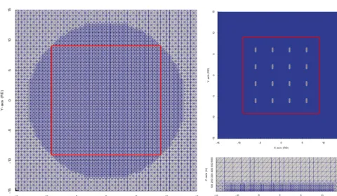
A coarse computational mesh of finite elements is gen-erated for the entire domain and then further refined within a circle that circumscribes the site boundaries, as shown in Fig. 2. For all tests presented here, the site boundary is as-sumed to be a square of side 18 RD centered in the com-putational domain. This area corresponds to a 6 RD spac-ing in streamwise and spanwise directions if 16 turbines are arranged in a regular grid. The resolution of the finite ele-ments used in the simulation can be quantified by the radius of a circle that circumscribes a single tetrahedral element, termed the circumradius. The mesh is refined such that the turbine rotor diameter is at least 4 times larger than the cir-cumradius of the finite elements within the wind plant site boundaries. The mesh is also stretched by a factor of 1.2 in the vertical direction in order to increase resolution near the bottom boundary. This results in a mesh with approximately 200 000 degrees of freedom.
Figure 1.A continuously differentiable modified exponential distribution is used to smoothly distribute the turbine forces and power pro-duction over the rotor swept area. The smoothing function is demonstrated for an 80 m rotor diameter turbine withγ=6 for 1-D and 2-D prototypes in panels(a)and(b)by taking conditional distributions ofϕ(x, y, z) in Eq. (12). The edge of the rotor disk is represented by vertical dashed red lines in panel(a). Panel(c)is a hub-height slice showing how a wind plant is represented as a summation of smoothed actuator disks.
Figure 2.Plan view of the computational mesh at hub height showing additional refinement around the wind turbine area (left), schematic of the computational domain showing the turbine locations used to initialize each optimization (top right), and side view of the mesh showing refinement below 2 rotor diameters (bottom right). The wind plant site constraint is shown as a red square in the plan view, and horizontal dimensions are normalized by the rotor diameter RD=80 m.
Simulations are performed for a range of different inflow directions and inflow speeds, corresponding to both ideal-ized and real-world wind roses and wind speed distributions. Steady-state solutions are found for each of the K wind states. We assume that the turbines are always yawed into the
rota-tion to the turbine coordinates corresponding to the inflow angle when calculating actuator disk forces. This rotation is included in the adjoint calculation and the resulting gradients are with respect to changes in the reference frame turbine co-ordinates. A weighted sum of the power production for each wind state (i.e., speed and direction) is performed based on the site wind speed distribution and wind rose, and the ad-joint gradient is calculated over the total power output, taking into account the layout rotation. Because the boundary con-ditions are part of a well-posed PDE used as an optimization constraint, this approach of rotating the layout is preferred to explicitly changing the inflow direction because the PDE constraint in the optimization is kept constant.
3.4 Gradient-based layout optimization process
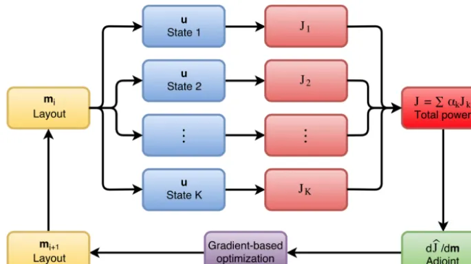
Figure 3 shows a schematic of the multi-state optimization workflow. The layout is optimized over all inflow states si-multaneously in a multilevel optimization process with re-spect to the total power output rather than in a sequential optimization process over each inflow separately. The basic optimization process is the following:
1. Begin with an initial layoutmi, which can be either a gridded or random layout of theNturbines.
2. Perform flow-field simulations for each of theKdesired wind states (corresponding to different wind speeds and directions obtained from either real or idealized wind roses and speed distributions).
3. Calculate the negative of the wind plant power,Jk, for each of theKwind states.
4. Calculate the objective function by taking a weighted sumJ =P
αkJkover allKwind states, whereαkis the relative probability of each wind state obtained from ei-ther a real or idealized wind rose and speed distribution.
5. Compute adjoint simulations for the forward simula-tions, and calculate the gradient of the reduced func-tional dJ /dm.ˆ
6. Use the gradient to perform a gradient-based optimiza-tion of the layout to obtainmi+1and go to step 2 above.
This process is repeated until the change in the objective function or its gradient falls below a user-defined threshold, which typically occurs in 30–50 iterations.
It should be noted that, because the optimization algo-rithm is gradient-based, it finds local rather than global min-ima in the total objective function J. The layout optimiza-tion problem can have many local minima, particularly with just a few inflow wind states. Starting with a regular grid-ded layout slightly smaller than the site constraint was gen-erally observed to produce reasonable results since none of the variables are initially constrained and a gridded layout is
often a “good enough” guess to be in the radius of conver-gence to the global optimum. This initial layout, used for all simulations described in the following, is shown in Fig. 2. However, gradient-based methods are still fundamentally lo-cal searches and cannot provide strong assurances of find-ing a global minima. We note that with many inflow states (i.e., for large K), the optimization problem actually be-comes more convex and convergence is achieved in fewer iterations. Additionally, running the optimization from many different starting configurations generated by random sam-pling or Latin hypercube samples can be used to further char-acterize the robustness of the minima.
3.5 Numerical implementation
The WindSE flow solver is implemented in a software pack-age calledFEniCS(Logg et al., 2012), which automates the solution of PDEs using the finite-element method.FEniCS
is written in Python and can be easily integrated with other Python-based systems engineering tools like WISDEM. The
FEniCSproject is based on theDOLFINproblem-solving environment and connects a number of useful components for the automatic discretization and solution of finite-element problems. These components include a form language that allows users to specify equations in variational form using a syntax that closely resembles their mathematical descrip-tion, automated compilers that generate finite-element forms for a chosen basis, and just-in-time compilation to C++to enhance computational speed.FEniCScan interface to com-mon HPC libraries such as PETSc and Trilinos for numerical linear algebra, ParMETIS and SCOTCH for domain decom-position, and MPI and OpenMP for parallelization.FEniCS
has been extensively tested and validated on a number of computational problems in solid and fluid mechanics, eigen-value problems, and coupled PDEs (Logg et al., 2012).
The description of finite-element problems as vari-ational forms in FEniCS lends itself to highly ab-stracted algorithmic differentiation. The software package
Figure 3.Schematic of the multilevel optimization process for a wind plant withKwind states (i.e., wind speeds and directions).
and automation across a wide range of PDE applications be-cause it avoids differentiating across low-level code where the mathematical and implementation details have been inter-mixed. Moreover,dolfin-adjointcan be implemented on unsteady and nonlinear PDEs, and can also be run in par-allel. It can directly interface to the optimization algorithms in SciPy and also contains routines for checking the correct-ness of adjoint gradients and checkpointing.
The 3-D RANS and continuity equations that form the PDE constraint in Eq. (7) are solved with a nonlinear New-ton solver in a coupled fashion using a mixed finite-element space with piecewise linear elements for both the velocity and pressure fields. To satisfy the Ladyzhenskaya–Babuška– Brezzi (LBB) (or inf-sup) compatibility condition (Brezzi and Fortin, 1991) with equal-order basis functions, we aug-ment the moaug-mentum equation with an additional pressure-stabilized Petrov–Galerkin term that weights the residual of the momentum equation by the gradient of the pressure test function. This pressure-based stabilization alleviates the saddle-point nature of the equal-order finite-element prob-lem (Donéa and Huerta, 2003) but still vanishes for the exact solution to the momentum equation. Each nonlinear solve is initialized with the base logarithmic velocity profile and the relative residual is converged to below 10−7with Newton’s method. The Newton solver uses Jacobians derived automat-ically withinFEniCSand linear systems are solved directly with the sparse, parallel solver MUMPS (Amestoy et al., 2000). The choice of equal-order piecewise linear mixed finite-element spaces differs from previous studies on wind and ocean turbine layout optimization in FEniCS (King et al., 2016; Funke et al., 2014) that used Taylor–Hood mixed finite-element spaces that are piecewise quadratic for the ve-locity field. The lower-order representation in this study was necessary when implementing a 3-D solver to keep the
to-tal degrees of freedom sufficiently low so that a direct linear algebra solver could be used.
The gradients obtained from dolfin-adjoint are used to optimize turbine locations with Python’s SciPy im-plementations of the sequential least-squares programming (SLSQP) or limited-memory Broyden–Fletcher–Goldfarb– Shanno (BFGS) algorithm with bounds (L-BFGS-B) algo-rithms. SLSQP is a gradient-based optimization algorithm that can also handle constraints (Nocedal and Wright, 1999). SLSQP minimizes a quadratic approximation to the objec-tive function at each optimization iteration, with a linear approximation of the constraints. The L-BFGS-B algorithm (Byrd et al., 1995) is a limited-memory version of the popular BFGS algorithm that approximates the inverse Hessian ma-trix used in quasi-Newton methods. We use the L-BFGS-B algorithm for simpler test cases without inter-turbine spacing constraints as in Sect. 4.2 and 4.3. In Sect. 4.4 we consider a real-world AEP optimization over a full wind rose and do enforce inter-turbine spacing constraints, which requires the use of the SLSQP algorithm. Gradients of the objective func-tion are provided bydolfin-adjointand gradients of the minimum turbine spacing constraint are calculated ana-lytically.
The forward and adjoint problems are parallelized with MPI and can be run on a desktop or in a high performance computing environment. The discrete adjoint calculation is automatically parallelized bydolfin-adjointif the for-ward model is run in parallel, which drastically simplifies code development.
4 Results
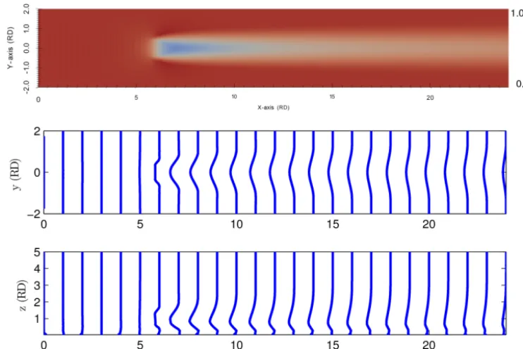
Figure 4.Flow past a single turbine obtained using the 3-D RANS flow solver. The top panel shows the velocity at hub height and the bottom two panels show profiles of the velocity deficit in horizontal and vertical planes passing through the center of the wind turbine rotor. Velocity deficits are relative to the respective profiles 3 RD upstream of the turbine and the velocities are normalized by the incoming hub-height velocity. Axes are in units of rotor diameter RD=80 m.
Figure 5.Hub-height velocity fields from the 3-D RANS solver used inWindSE show good qualitative agreement with time-averaged LES velocity fields of similar wind plants reported in the literature (Wu and Porté-Agel, 2013), even in the case of very deep wind plants. Velocities are normalized by incoming hub-height speed of 8 m s−1and distances are normalized by the 80 m rotor diameter.
very deep wind plant in order to demonstrate that the RANS flow solver accurately captures wind turbine wakes, thereby providing confidence that subsequent layout optimizations are performed according to the correct flow physics. Second, we optimize a 16-turbine wind plant using wind roses with evenly weighted wind directions and a constant wind speed of 8 m s−1in order to demonstrate new layout insights and optimization heuristics when accounting for nonlinear flow effects with a high-fidelity model. Third, we optimize a 16-turbine wind plant using unevenly weighted wind roses that exhibit complex directional preferences, again with a con-stant wind speed of 8 m s−1. Finally, we perform a full AEP optimization using data from the M2 meteorological tower
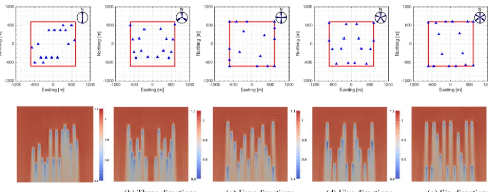
Figure 6.Optimal layouts (top row) and flow fields (bottom row) for five test cases with an increasing number of evenly weighted inflow directions. The wind roses in the upper right corner of each layout plot show the inflow directions used in the optimization. The blue triangles show the optimized turbine locations and the red square indicates the site boundaries. The velocities are normalized by the hub-height inflow velocity, which is 8 m s−1in these simulations. Each of the flow fields are shown for a wind that blows from the north.
Table 1.Relative efficiency of power production from the test cases compared to 16 turbines with no wake effects. Results from a “naïve” case with two parallel turbine rows and no layout optimization are also included to demonstrate the improvements achieved by the layout optimization.
All unwaked Two-dir. naïve Two-dir. opt. Three-dir. opt. Four-dir. opt. Five-dir. opt. Six-dir. opt.
1.0 0.833 0.9854 0.953 0.960 0.948 0.974
4.1 RANS model testing
As a test of the qualitative performance of the RANS flow solver, WindSEwas used to simulate flow fields for both a single turbine and a deep wind plant. Figure 4 shows verti-cal and horizontal velocity profiles in the wake of a single wind turbine. Consistent with theoretical expectations and previous results, a logarithmic velocity profile is observed in the undisturbed flow upstream of the turbine, a Gaussian ve-locity deficit is observed in the turbine wake, and a gradual wake recovery is observed with increasing distance down-stream from the turbine. Moreover, a slight speedup around the edges of the wake is observed near the turbine rotor – such speedups are not captured by traditional linear wake flow models and appear here due to the use of the higher-fidelity RANS flow solver, which more accurately captures nonlinear flow physics. Figure 5 shows the velocity field from a simulation of a wind plant with 10 turbine rows per-pendicular to the incoming wind direction. This flow field qualitatively agrees with time-averaged LES results reported by Wu and Porté-Agel (2013).
The results presented in this section are only intended to demonstrate the qualitative agreement of the RANS solver with prior high-fidelity studies and analytical wake theory. This demonstrates that the present flow solver captures a
rea-sonable level of fidelity to introduce the adjoint optimiza-tion framework. A detailed turbulence model verificaoptimiza-tion and validation is beyond the scope of this study as we are in-stead focused on the integration of the model into a flexible and automated adjoint optimization framework. A compre-hensive study on the implementation of more sophisticated turbulence models within the WindSE framework is left for future research.
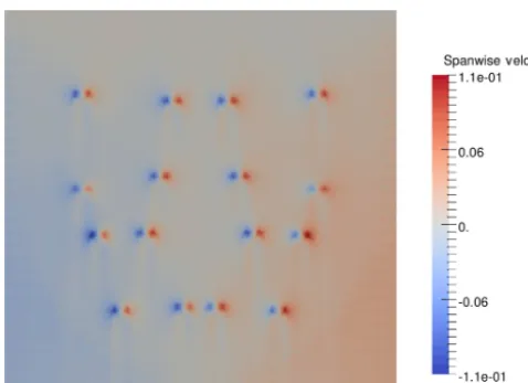
Figure 7. Spanwise velocities produced by the optimized layout found in the five-inflow-direction case shown in Fig. 6d. The span-wise velocity is normalized by the hub-height inflow velocity, indi-cating strong curvature at the rotor and a slight overall deflection of the flow away from the center of the wind plant.
Figure 6 shows that optimal layouts are symmetric about a rotation or reflection when the wind directions are evenly weighted. For the two-direction and six-direction cases shown in Fig. 6a and e, the layout is symmetric about a 180◦ rotation and for the four-direction case shown in Fig. 6c, the layout is symmetric about a 90◦rotation. For odd numbers of inflow directions, Fig. 6b and d show that optimal layouts are symmetric about a horizontal reflection across the north– south axis. The rotational and reflectional symmetries of the layouts for evenly weighted, uniform speed wind roses are useful heuristics for checking the flow solver and optimiza-tion results.
The flow fields shown in Fig. 6 indicate that the RANS solver captures flow curvature due to nonlinear turbulent transport effects and pressure increases upwind of the ro-tor disk. These effects are neglected when superimposing a wake deficit on a flow field obtained from a linear model, as is typically done in many industry-standard optimization frameworks. The flow curvature results in local speedup ef-fects between two turbines, or just outside a wake, that down-wind turbines take advantage of in strongly directional down-wind roses. This effect is further demonstrated in Fig. 7, which shows nonzero spanwise velocities generated by the flow curving around the turbines. This curvature is responsible for the “staggered” appearance of many of the layouts in Fig. 6 where the optimizer takes advantage of these local speedups. Because the power production scales with the cube of the wind speed, these small speedups can have a strong nonlinear effect on the power output. This speedup effect due to flow curvature is particularly enhanced in 2-D, but is still present in the 3-D simulations.
Flow curvature also affects the propagation and interac-tion of the turbine wakes. Wakes near the edge of the plant
are slightly deflected away from the plant center and reflect the overall spreading of the flow streamlines. This curva-ture can be observed near the edges of the plant in the cases shown in Fig. 6. Such curvature is again not captured by en-gineering wake models which prescribe wakes that always travel perpendicular to the rotor. Additionally, the wakes are pinched, curved, or merged when encountering speedups around downwind turbines or other wakes. The RANS flow solver accounts for the effects of other turbines and their wakes on the expansion and dissipation of wakes beyond what is accounted for in prescribed wake models. The de-flection and curvature of wakes likely has important ramifi-cations for yaw control strategies that attempt to steer wakes away from downwind turbines.
It is emphasized that the results in Fig. 6 show that the optimizer does not place turbines in straight rows perpendic-ular to a single predominant wind direction or in a regperpendic-ularly spaced grid for these evenly weighted wind rose cases. In-stead, the turbines are placed closer together and staggered to take advantage of local speedups between laterally placed turbines. This is a different strategy than the maximized spac-ing found when optimizspac-ing with linear flow models and pre-scribed wakes, and is likely sensitive to the number and size of wind direction bins.
We compared the optimized layout for two inflow direc-tions shown in Fig. 6a to a case with two parallel rows of turbines aligned perpendicular to the inflow directions and with maximal spacing between the rows as allowed by the site constraints. This “naïve” strategy is often found when using linear flow models. The optimized layout increases power production by 18.4 % over the “naïve” layout due to the strongly directional speedups in this case. We also exam-ined the power production of the test cases when normalized by the total power available if all turbines were unwaked, shown in Table 1. The optimized layouts substantially re-duce, but do not entirely eliminate, the wake losses.
4.3 Layout optimization with unevenly weighted wind roses
In the previous section, each inflow direction was given an equal weight (i.e.,αk) in creating the total objective function J. However, real-world wind roses are seldom so simple and typically have several preferred wind directions, with many other less dominant directions. Here we demonstrate opti-mization of a 16-turbine layout using the same computational domain and setup as in the previous section, but with un-evenly weighted wind roses that have two and three dominant directions. Once again, in both cases we assume a constant 8 m s−1wind speed and do not enforce inter-turbine spacing constraints.
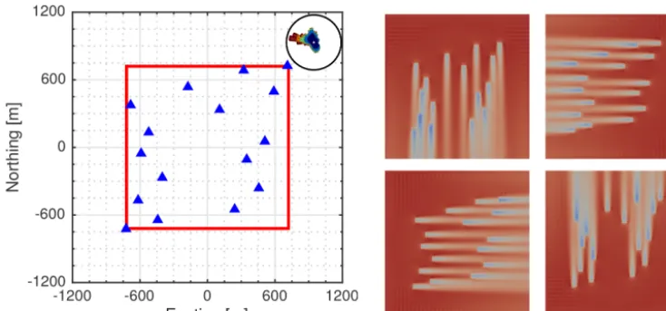
Figure 8.Optimal layout (left) and flow field (right) for the boomerang test case with the wind rose binned into 36 inflow directions and a uniform hub-height velocity of 8 m s−1. The wind rose is shown in the upper right corner of the left panel, and the site boundary is shown by a solid red line. Turbine locations are denoted by blue triangles. The flow field in the right panel is normalized by the incoming hub-height velocity of 8 m s−1and shows results for an inflow wind from the south.
Figure 9.Optimal layout (left) and flow field (right) for the NWTC M2 8 m s−1test case with the wind rose binned into 36 inflow directions. The wind rose is shown in the upper right corner of the left panel, and the site boundary is shown by a solid red line. Turbine locations are denoted by blue triangles. The flow field in the right panel is normalized by the incoming hub-height velocity of 8 m s−1and shows results for an inflow wind from the west.
boomerang, as shown in Fig. 8. Compared to the initial uni-form gridded layout (see Fig. 2), the optimized layout shown in Fig. 8 improves power production by 9.4 %. Despite the uneven weighting of the wind rose, the resulting flow field in the right panel of Fig. 8 once again conforms to many of the heuristics outlined in the previous section, including turbines that take advantage of local speedups between upstream tur-bines and slight flow curvature at the edge of the plant.
The second wind rose considered is given by the direc-tional distribution of 8 m s−1wind speeds from the M2 mast at NWTC (Jager and Andreas, 1996), as shown in Fig. 9. The wind rose is constructed from publicly available data recorded over the 2015 calendar year. For this wind speed, the wind rose has three prominent directions roughly aligned with inflow from the north, south, and west, along with
Figure 10.Optimal layout (top left) and flow fields resulting from a full AEP optimization using data from the M2 mast at NWTC. Differ-ences in both wind speed and wind direction are accounted for in the optimization, and the wind rose used is shown in the top right corner of the layout plot. In the top left panel, the site boundary is shown by a solid red line and turbine locations are denoted by blue triangles. Flow fields are shown for inflow winds from the north (top left), east (top right), south (bottom right), and west (bottom left).
4.4 Layout optimization based on annual energy production
As a final demonstration of the power and flexibility of
WindSE, we optimize a 16-turbine wind plant based on the full AEP from real-world site data. In this case, wind states corresponding to both different wind speeds and wind direc-tions are considered, instead of simply considering a single uniform wind speed as in the tests described in the previous two sections. Data are once again used from the M2 mast at NWTC (Jager and Andreas, 1996), and distributions are formed by binning the data into 36 wind directions and 5 wind speed classes centered on 4, 6, 8, 10, and 12 m s−1, giv-ing a total ofK=180 possible wind states in the analysis. Wind states that occurred less than 0.2 % of the time were neglected in the optimization, reducing the total number of states considered to 99. We further enforce a minimum inter-turbine spacingDminof 3 times the rotor diameter.
As shown in Fig. 10, the wind rose for the M2 mast is predominately distributed along the west-northwest direc-tion, with secondary influences from the north and south. The highest wind speeds are also observed for winds from the west-northwest, and so it can be anticipated that a full AEP optimization will result in a layout that is preferen-tially suited for winds that blow from this direction. This is indeed the case, as shown in the final optimized layout in Fig. 10. The turbines are loosely arranged in two north– south rows that result in relatively large separations between upstream and downstream turbines when the wind is from the west-northwest. As with other tests for evenly and unevenly weighted wind roses with uniform wind speeds, the turbines in the full AEP optimization are staggered with respect to each other in order to take advantage of local speedups be-tween upwind turbines. The resulting optimized layout
im-proves AEP by 8.6 % compared to the initial regular gridded layout shown in Fig. 2.
It should be noted that despite the predominant high-speed winds from the west-northwest, the turbines in the north– south rows shown in Fig. 10 do not each fall perfectly on the site boundaries. That is, if only winds from the west-northwest were included in the analysis, one might naïvely place all turbines along the upstream and downstream site boundaries in order to maximize the separation between tur-bines in the direction of the dominant wind. However, since other wind directions are also included in the analysis, the fi-nal optimal layout is more complicated and ensures some de-gree of turbine staggering in the east–west direction to take advantage of local speedups and minimize wake losses when the wind blows from the north or south. It is also emphasized that simply by accounting for the full AEP in the optimiza-tion, the optimal layout in Fig. 10 is substantially different from the optimal layout shown in Fig. 9, where only a single uniform wind speed was considered.
5 Summary and conclusions
first-principles flow model without running expensive LES for tuning purposes. The results presented in this paper are achieved at a relatively low computational cost as all opti-mization results were obtained on a single workstation with a six-core Intel Xeon processor and 32 GB of memory.
The results presented in this paper show that the nonlinear flow effects leading to wake curvature and local speedups are significant when optimizing over a few prominent wind directions. We find consistent rotational symmetry in the op-timal layouts with evenly weighted inflow directions, sug-gesting that evenly weighted wind roses may be useful di-agnostic tests for wind plant optimization. As the wind rose is refined into more bin directions, the optimizer is able to take advantage of prominent wind directions and increase en-ergy production. As the number of wind direction and inflow speed combinations increases,WindSEis able to perform a full AEP optimization and achieve sizable gains of almost 9 % compared to initial gridded layouts. In the full AEP op-timization, the optimizer emphasizes the high speed winds from the west-northwest, since these winds contain the most energy. However, rather than aligning the turbines into rows perpendicular to the incoming wind, the turbines are offset within the general row structure. This is beneficial when the wind is blowing parallel to the row, which is the most com-mon secondary wind direction. It also allows the turbines to take advantage of slight speedup effects around the edges of the wake from upstream turbines. The gradient-based tech-niques used in this study are inherently constrained to a lo-cal search, however, and further research is needed to assess what types of initial layouts are needed to draw conclusions about global optima.
A number of different future studies utilizing WindSE
can be imagined. Because the adjoint approach is insensi-tive to the number of control variables, coupled optimization of turbine locations, hub height, rotor diameter, control set-tings, etc. can be considered. The flow curvature captured in
WindSEis observed to deflect or modify turbine wakes and will likely have important implications in yaw control opti-mization applications. The high level of abstraction and au-tomation also makesWindSEa useful framework for study-ing the effects of different turbulence closure models on opti-mal layouts. We further intend to compare layouts optimized using WindSEand linear flow models by testing both lay-outs using LES. Additionally, the finite-element method used inWindSEis, in principle, also well suited to examining lay-out optimization in the presence of terrain-induced complex flows. Finally, the integration ofWindSEwithin NREL sys-tems engineering tools will enable economic analysis and a consideration of LCOE alongside AEP in future optimization studies.
Data availability. Simulations were performed using the WindSE code that will be made available through NREL’s WISDEM soft-ware tool (Dykes et al., 2014), and can be accessed at https://nwtc.
nrel.gov/WISDEM. The NWTC wind data used for layout opti-mizations in Sect. 4.3 and 4.4 are available at https://www.nrel.gov/ midc/nwtc_m2/ (Jager and Andreas, 1996).
Competing interests. The authors declare that they have no con-flict of interest.
Acknowledgements. This work was supported by award UGA-0-41026-70 through the Alliance Partner University Program in partnership with the National Renewable Energy Laboratory.
Edited by: J. Peinke
Reviewed by: three anonymous referees
References
Ainslie, J.: Calculating the flowfield in the wake of wind tur-bines, J. Wind Eng. Ind. Aerod., 27, 213–224, doi:10.1016/0167-6105(88)90037-2, 1988.
Amestoy, P. R., Duff, I. S., and L’Excellent, J. Y.: Multifrontal parallel distributed symmetric and unsymmetric solvers, Com-put. Method. Appl. M., 184, 501–520, doi:10.1016/S0045-7825(99)00242-X, 2000.
Barthelmie, R. J., Hansen, K., Frandsen, S. T., Rathmann, O., Schepers, J. G., Schlez, W., Phillips, J., Rados, K., Zervos, A., Politis, E. S., and Chaviaropoulos, P. K.: Modelling and measur-ing flow and wind turbine wakes in large wind farms offshore, Wind Energy, 12, 431–444, doi:10.1002/we.348, 2009. Boersma, S., Gebraad, P., Vali, M., Doekemeijer, B., and
van Wingerden, J.: A control-oriented dynamic wind farm flow model: “WFSim”, J. Phys. Conf. Ser., 753, 032005, doi:10.1088/1742-6596/753/3/032005, 2016.
Bokharaie, V. S., Bauweraerts, P., and Meyers, J.: Wind-farm layout optimisation using a hybrid Jensen-LES approach, Wind Energ. Sci., 1, 311–325, doi:10.5194/wes-1-311-2016, 2016.
Brezzi, F. and Fortin, M. (Eds.): Mixed and Hybrid Finite Ele-ment Methods, Springer Series in Computational Mathematics, Springer New York, New York, NY, 15, ISBN 978-1-4612-7824-5, 1991.
Burton, T., Sharpe, D., Jenkins, N., and Bossanyi, E.: Wind en-ergy handbook, John Wiley & Sons, Chichester, West Sussex, 2nd Edn., 2011.
Byrd, R. H., Lu, P., Nocedal, J., and Zhu, C.: A Limited Memory Algorithm for Bound Constrained Optimization, SIAM J. Sci. Comput., 16, 1190–1208, doi:10.1137/0916069, 1995.
Cabezón, D., Migoya, E., and Crespo, A.: Comparison of turbulence models for the computational fluid dynamics simulation of wind turbine wakes in the atmospheric boundary layer, Wind Energy, 14, 909–921, doi:10.1002/we.516, 2011.
Calaf, M., Meneveau, C., and Meyers, J.: Large eddy simulation study of fully developed wind-turbine array boundary layers, Phys. Fluids, 22, 015110-1–015110-16, doi:10.1063/1.3291077, 2010.
Chowdhury, S., Zhang, J., Messac, A., and Castillo, L.: Unrestricted wind farm layout optimization (UWFLO): Investigating key fac-tors influencing the maximum power generation, Renew. Energ., 38, 16–30, doi:10.1016/j.renene.2011.06.033, 2012.
Churchfield, M. J., Lee, S., Michalakes, J., and Moriarty, P. J.: A numerical study of the effects of atmospheric and wake turbulence on wind turbine dynamics, J. Turbul., 13, 1–32, doi:10.1080/14685248.2012.668191, 2012.
Crespo, A., Hernández, J., and Frandsen, S.: Survey of modelling methods for wind turbine wakes and wind farms, Wind Energy, 2, 1–24, doi:10.1002/(SICI)1099-1824(199901/03)2:1<1::AID-WE16>3.0.CO;2-7, 1999.
Donéa, J. and Huerta, A.: Finite element methods for flow problems, Wiley, Chichester, Hoboken, NJ, 2003.
Du Pont, B. L. and Cagan, J.: An Extended Pattern Search Ap-proach to Wind Farm Layout Optimization, J. Mech. Design, 134, 081002, doi:10.1115/1.4006997, 2012.
Dykes, K., Ning, A., King, R., Graf, P., Scott, G., and Veers, P. S.: Sensitivity Analysis of Wind Plant Performance to Key Turbine Design Parameters: A Systems Engineering Approach, American Institute of Aeronautics and Astronautics, 1087, 1–25 doi:10.2514/6.2014-1087, 2014.
El Kasmi, A. and Masson, C.: An extended model for turbulent flow through horizontal-axis wind turbines, J. Wind Eng. Ind. Aerod., 96, 103–122, doi:10.1016/j.jweia.2007.03.007, 2008.
Farrell, P. E., Ham, D. A., Funke, S. W., and Rognes, M. E.: Au-tomated Derivation of the Adjoint of High-Level Transient Fi-nite Element Programs, SIAM J. Sci. Comput., 35, C369–C393, doi:10.1137/120873558, 2013.
Fitch, A. C., Olson, J. B., Lundquist, J. K., Dudhia, J., Gupta, A. K., Michalakes, J., and Barstad, I.: Local and Mesoscale Impacts of Wind Farms as Parameterized in a Mesoscale NWP Model, Mon. Rev., 140, 3017–3038, doi:10.1175/MWR-D-11-00352.1, 2012. Fleming, P. A., Ning, A., Gebraad, P. M. O., and Dykes, K.: Wind plant system engineering through optimization of layout and yaw control: Wind plant system engineering, Wind Energy, 19, 329– 344, doi:10.1002/we.1836, 2016.
Funke, S., Farrell, P., and Piggott, M.: Tidal turbine array optimi-sation using the adjoint approach, Renew. Energ., 63, 658–673, doi:10.1016/j.renene.2013.09.031, 2014.
Gebraad, P. M. O., Teeuwisse, F. W., van Wingerden, J. W., Flem-ing, P. A., Ruben, S. D., Marden, J. R., and Pao, L. Y.: Wind plant power optimization through yaw control using a parametric model for wake effects-a CFD simulation study: Wind plant op-timization by yaw control using a parametric wake model, Wind Energy, 19, 95–114, doi:10.1002/we.1822, 2016.
Giannakoglou, K. C. and Papadimitriou, D. I.: Adjoint methods for shape optimization, in: Optimization and computational fluid dynamics, Springer, 79–108, http://link.springer.com/chapter/10. 1007/978-3-540-72153-6_4, last access: 8 December 2008. Giles, M. B. and Pierce, N. A.: An introduction to the adjoint
ap-proach to design, Flow Turbul. Combust., 65, 393–415, 2000. Goit, J., Munters, W., and Meyers, J.: Optimal Coordinated
Con-trol of Power Extraction in LES of a Wind Farm with Entrance Effects, Energies, 9, 29, doi:10.3390/en9010029, 2016. Goit, J. P. and Meyers, J.: Optimal control of energy
extrac-tion in wind-farm boundary layers, J. Fluid Mech., 768, 5–50, doi:10.1017/jfm.2015.70, 2015.
González, J. S., Gonzalez Rodriguez, A. G., Mora, J. C., Santos, J. R., and Payan, M. B.: Optimization of wind farm turbines lay-out using an evolutive algorithm, Renew. Energ., 35, 1671–1681, doi:10.1016/j.renene.2010.01.010, 2010.
Herbert-Acero, J., Probst, O., Réthoré, P.-E., Larsen, G., and Castillo-Villar, K.: A Review of Methodological Approaches for the Design and Optimization of Wind Farms, Energies, 7, 6930– 7016, doi:10.3390/en7116930, 2014.
Heywood, J. G., Rannacher, R., and Turek, S.: Artificial boundaries and flux and pressure conditions for the incompressible Navier-Stokes equations, Int. J. Numer. Meth. Fl., 22, 325–352, 1996. Hinze, M., Pinnau, R., Ulbrich, M., and Ulbrich, S.: Optimization
with PDE Constraints, Mathematical Modelling: Theory and Ap-plications, Springer, 2009, 23, 2009.
Iungo, G. V., Viola, F., Ciri, U., Leonardi, S., and Rotea, M.: Re-duced order model for optimization of power production from a wind farm, American Institute of Aeronautics and Astronautics, 2200, 1–9, doi:10.2514/6.2016-2200, 2016.
Jackson, P. S. and Hunt, J. C. R.: Turbulent wind flow over a low hill, Q. J. Roy. Meteor. Soc., 101, 929–955, doi:10.1002/qj.49710143015, 1975.
Jager, D. and Andreas, A.: NREL National Wind Technology Cen-ter (NWTC): M2 Tower; Boulder, Colorado (Data), https://www. nrel.gov/midc/nwtc_m2/ (last access: 12 May 2016), 1996. Jameson, A.: Aerodynamic shape optimization using the adjoint
method, Lectures at the Von Karman Institute, Brussels, http: //aero-comlab.stanford.edu/Papers/jameson.vki03.pdf (last ac-cess: 26 July 2013), 2003.
Jensen, N. O.: A note on wind generator interaction, Risø-M No. 2411 Risø National Laboratory Roskilde, 1–16, http://orbit. dtu.dk/files/55857682/ris_m_2411.pdf (last access: 28 February 2017), 1983.
Jimenez, A., Crespo, A., Migoya, E., and Garcia, J.: Advances in large-eddy simulation of a wind turbine wake, J. Phys. Conf. Ser., 75, 012041, doi:10.1088/1742-6596/75/1/012041, 2007. King, R., Hamlington, P., Dykes, K., and Graf, P.: Adjoint
Opti-mization of wind Farm Layouts for Systems Engineering Anal-ysis, American Institute of Aeronautics and Astronautics, vol. AIAA 2016-2199, doi:10.2514/6.2016-2199, 2016.
Kusiak, A. and Song, Z.: Design of wind farm layout for maximum wind energy capture, Renew. Energ., 35, 685–694, doi:10.1016/j.renene.2009.08.019, 2010.
Kwong, W. Y., Zhang, P. Y., Romero, D., Moran, J., Morgenroth, M., and Amon, C.: Wind farm layout optimization considering energy generation and noise propagation, in: ASME 2012 Inter-national Design Engineering Technical Conferences and Com-puters and Information in Engineering Conference, American Society of Mechanical Engineers, DETC2012-71478, 323–332, doi:10.1115/DETC2012-71478, 2012.
Larsen, G. C., Aagaard Madsen, H., Troldborg, N., Larsen, T. J., Réthoré, P.-E., Fuglsang, P., Ott, S., Mann, J., Buhl, T., Nielsen, M. et al.: TOPFARM-next generation design tool for opti-misation of wind farm topology and operation, Tech. Rep. Risø-R-1805(EN), Risø DTU Naitonal Laboratory for Sustain-able Energy, http://forskningsbasen.deff.dk/Share.external?sp= S14b3124a-fef2-4c0b-8f80-6dae7c10ddd2&sp=Sdtu (last ac-cess: 28 February 2017), 2011.
Lec-ture Notes in Computational Science and Engineering, Springer Berlin Heidelberg, Berlin, Heidelberg, 84, http://link.springer. com/10.1007/978-3-642-23099-8, 2012.
Luchini, P. and Bottaro, A.: Adjoint Equations in Stability Analy-sis, Annu. Rev. Fluid Mech., 46, 493–517, doi:10.1146/annurev-fluid-010313-141253, 2014.
Marden, J. R., Ruben, S. D., and Pao, L. Y.: A Model-Free Approach to Wind Farm Control Using Game The-oretic Methods, IEEE T. Contr. Syst. T., 21, 1207–1214, doi:10.1109/TCST.2013.2257780, 2013.
Martins, J. R. R. A. and Hwang, J. T.: Review and Unifi-cation of Methods for Computing Derivatives of Multidis-ciplinary Computational Models, AIAA J., 51, 2582–2599, doi:10.2514/1.J052184, 2013.
Meyers, J. and Meneveau, C.: Optimal turbine spacing in fully de-veloped wind farm boundary layers, Wind Energy, 15, 305–317, doi:10.1002/we.469, 2012.
Mirocha, J. D., Kosovic, B., Aitken, M. L., and Lundquist, J. K.: Im-plementation of a generalized actuator disk wind turbine model into the weather research and forecasting model for large-eddy simulation applications, Journal of Renewable and Sustainable Energy, 6, 013104, doi:10.1063/1.4861061, 2014.
Nocedal, J. and Wright, S. J.: Numerical optimization, Springer, New York, ISBN: 978-0-387-30303-1, 1999.
Porté-Agel, F., Wu, Y.-T., Lu, H., and Conzemius, R. J.: Large-eddy simulation of atmospheric boundary layer flow through wind tur-bines and wind farms, J. Wind Eng. Ind. Aerod., 99, 154–168, doi:10.1016/j.jweia.2011.01.011, 2011.
Sanderse, B., Pijl, S., and Koren, B.: Review of computational fluid dynamics for wind turbine wake aerodynamics, Wind Energy, 14, 799–819, doi:10.1002/we.458, 2011.
van der Laan, M. P., Sørensen, N. N., Réthoré, P.-E., Mann, J., Kelly, M. C., Troldborg, N., Hansen, K. S., and Murcia, J. P.: The k- -fP model applied to wind farms, Wind Energy, 18, 2065–2084, doi:10.100/we.1804, 2015a.
van der Laan, M. P., Sørensen, N. N., Réthoré, P.-E., Mann, J., Kelly, M. C., Troldborg, N., Schepers, J. G., and Machefaux, E.: An im-proved k-model applied to a wind turbine wake in atmospheric turbulence, Wind Energy, 18, 889–907, doi:10.1002/we.1736, 2015b.
Walmsley, J. L., Taylor, P. A., and Keith, T.: A simple model of neu-trally stratified boundary-layer flow over complex terrain with surface roughness modulations (MS3DJH/3R), Bound.-Lay. Me-teorol., 36, 157–186, doi:10.1007/BF00117466, 1986.
Wilcox, D. C.: Turbulence modeling for CFD, DCW Industries, La Cãnada, Calif, 3rd Edn., 2006.
Wu, Y.-T. and Porté-Agel, F.: Large-Eddy Simulation of Wind-Turbine Wakes: Evaluation of Wind-Turbine Parametrisations, Bound.-Lay. Meteorol., 138, 345–366, doi:10.1007/s10546-010-9569-x, 2010.