Http://www.ijetmr.com©International Journal of Engineering Technologies and Management Research [1]
COMPARATIVE ANALYSIS OF SUPERPIXEL SEGMENTATION
METHODS
SumitKaur *1, Dr. R.K Bansal 2 *1
Research Scholar, Gurukashi University, TalwandiSaboo, India 2
Dean Research, Gurukashi University, TalwandiSaboo, India
Abstract:
Superpixel segmentation showed to be a useful preprocessing step in many computer vision applications. Superpixel’s purpose is to reduce the redundancy in the image and increase efficiency from the point of view of the next processing task. This led to a variety of algorithms to compute superpixel segmentations, each with individual strengths and weaknesses. Many methods for the computation of superpixels were already presented. A drawback of most of these methods is their high computational complexity and hence high computational time consumption. K mean based SLIC method shows better performance as compare to other while evaluating on the bases of under segmentation error and boundary recall, etc parameters.
Keywords: Image segmentation; Morphological Processing; Superpixel.
Cite This Article: SumitKaur, and Dr. R.K Bansal. (2018). “COMPARATIVE ANALYSIS OF SUPERPIXEL SEGMENTATION METHODS.” International Journal of Engineering Technologies and Management Research, 5(3), 1-9. DOI: 10.29121/ijetmr.v5.i3.2018.172.
1. Introduction
Http://www.ijetmr.com©International Journal of Engineering Technologies and Management Research [2] sentence, superpixels are an over-segmentation of an image - or seen the other way around a perceptual grouping of pixels. Instead of finding the few (e.g one to five) foreground segments that correspond to objects, superpixel segmentation algorithms split the image into typically 25 to 2500 segments. The objective of this over-segmentation is a partitioning of the image such that no superpixel is split by an object boundary, while objects may be divided into multiple superpixels. This way, the object outlines can be recovered from the superpixel boundaries at later processing stages. Such segmentations are sometimes also coined multipurpose image segmentations.
There are many approaches to generate superpixels, each with its own advantages and drawbacks that may be better suited to a particular application. For example, if adherence to image boundaries is of paramount importance, the graph-based method of [2] may be an ideal choice. However, if superpixels are to be used to build a graph, a method that produces a more regular lattice, such as [3], is probably a better choice. While it is difficult to define what constitutes an ideal approach for all applications, we believe the following properties are generally desirable:
1) Superpixels should adhere well to image boundaries.
2) When used to reduce computational complexity as a preprocessing step, superpixels should be fast to compute, memory efficient, and simple to use.
3) When used for segmentation purposes, superpixels should both increase the speed and improve the quality of the results.
Downsides of using superpixel segmentation as preprocessing step are the computational effort for the computation of superpixels and more importantly the risk of losing meaningful image edges by placing them inside a superpixel. Depending on the application and the used superpixel algorithm, subsequent processing steps can struggle with a non-lattice arrangement of the superpixels. Therefore, the careful choice of the superpixel algorithm and its parameters for the particular application are crucial.
2. Applications
2.1.Semantic Segmentation
Semantic segmentation aims at assigning pre-defined class labels to every pixel in an image. One of the most successful frameworks for this task models the problem as an energy minimization of a conditional random field (CRF) [6], [7]. By working directly on the superpixel level instead of the pixel level, the number of nodes in the CRF is significantly reduced (typically from 105 to 102 per image [7]). Therefore, the inference algorithm converges drastically faster [7]. Following [8], we use the method of [9] to evaluate superpixel algorithms on the MSRC-21 database [10]. The original annotations of MSRC-21 are quite imprecise and in order to get reliable results, we use an accurate version provided by [11]. All settings of [9] are kept constant for all superpixel methods.
2.2.Saliency Detection
Http://www.ijetmr.com©International Journal of Engineering Technologies and Management Research [3] can be designed in a single-layer (SCA) or multi-layer (MCA) fashion. It’s shown in [12] that MCA improves saliency detection accuracy significantly compared to SCA by fusing multiple saliency detection methods. Here we demonstrate that improvement can also be achieved by fusing multi-scale segmentation. SH shows striking advantages for this task as generating the most accurate saliency maps and reducing computational cost significantly.
2.3.Stereo Matching
To demonstrate the usefulness of tree structure provided by SH, we integrate it with the non-local cost aggregation method [13] for stereo matching. Different from traditional non-local stereo methods, [13] performs cost aggregation over the entire image with a MST in a non-local manner. The method is computationally very efficient, with a complexity comparable to uniform box filtering and also shows edge-preserving and non-local properties. Following [14], we quantitatively evaluate the aggregation accuracy with MST, FH, ERS and our SH on 19 Middlebury data sets. All the methods use the same cost volume and do not employ any post-processing. The subscripts represent relative rank of the methods on each data set. As expected, all segmentation-based structures improve the basic MST. The performance of proposed SH is higher than the other tree structures. It obtains the lowest average error rate and the highest average ranking. SH achieves the most accurate results on 13 (out of 19) datasets.
3. Existing Techniques
A lot of superpixel algorithms have been proposed in the last decade. Therefore, it is difficult to select appropriate approaches for specific applications. In this paper different algorithms available for superpixel segmentation will be reviewed based on their performances. Algorithms for generating superpixels can be broadly categorized as either graph-based or gradient ascent methods.
3.1.Graph Based Algorithms
Http://www.ijetmr.com©International Journal of Engineering Technologies and Management Research [4] of a partition of V into subsets A and B as a fraction of the total edge connections to all the nodes in the graph:
𝑁𝐶(𝐴, 𝐵) = 𝑐𝑢𝑡(𝐴,𝐵)
𝑎𝑠𝑠𝑜𝑐(𝐴,𝑉)+
𝑐𝑢𝑡(𝐴,𝐵)
𝑎𝑠𝑠𝑜𝑐(𝐵,𝑉) (1)
Where
𝑎𝑠𝑠𝑜𝑐(𝐴, 𝑉) = ∑𝑎∈𝐴,𝑣∈𝑉𝑤(𝑎, 𝑣) (2)
is the sum of weights from the subset of nodes A to all nodes in the graph. This definition penalizes small sets of vertices since their cut value “almost certainly” becomes a high fraction of their total sum of connection weights.
Felzenszwalb-Huttenlocher Segmentation (FH): an alternative graph-based approach that has been applied to generate superpixels. It performs an agglomerative clustering of pixels as nodes on a graph, such that each superpixel is the minimum spanning tree of the constituent pixels. FH adheres well to image boundaries in practice, but produces superpixels with very irregular sizes and shapes. They define a predicate for measuring the evidence of a boundary between two regions and present an implementation in a greedy algorithm that also satisfies global properties. Its goal is to preserve details in low variability image regions and ignore details in high-variability image regions.
SL: Moore et al. propose a method to generate superpixels that conform to a grid by finding optimal paths, or seams, that split the image into smaller vertical or horizontal regions [17]. Optimal paths are found using a graph cuts method similar to Seam Carving [18]. While the complexity of SL08 is O (N 3 2 log N) according to the authors, this does not account for the pre-computed boundary maps, which strongly influence the quality and speed of the output.
Vekslersuperpixels (VEK): Veksler et al. [2010] propose another graph cut based approach for superpixel tessellation that focuses on regular partition. They formulate the segmentation problem as an energy minimization problem that explicitly encourages regular superpixels.Superpixels are obtained by stitching together overlapping image patches such that each pixel belongs to only one of the overlapping regions.
3.2.Gradient –Ascent Based
Http://www.ijetmr.com©International Journal of Engineering Technologies and Management Research [5] the algorithm follows the gradient of the density to assign each pixel to a mode. The modes represent the final segments.
Marker-Controlled Watershed Segmentation (WS): The watershed approach [21] performs a gradient ascent starting from local minima to produce watersheds, lines that separate catchment basins. The resulting superpixels are often highly irregular in size and shape, and do not exhibit good boundary adherence. The approach of [21] is relatively fast (O (N log N) complexity), but does not offer control over the amount of superpixels or their compactness.
Mean Shift (MS): In [22], mean shift, an iterative mode-seeking procedure for locating local maxima of a density function, is applied to find modes in the color or intensity feature space of an image. Pixels that converge to the same mode define the superpixels. MS02 is an older approach, producing irregularly shaped superpixels of non-uniform size. It is O (N 2) complex, making it relatively slow and does not offer direct control over the amount, size, or compactness of superpixels.
Turbopixel Segmentation (TP): Turbopixels is an algorithm inspired by active contours [20]. After selecting initial superpixel centers, each superpixel is grown by the means of an evolving contour. TP09 produced some of the most compact and consistently sized superpixels, it fared the worst among all methods in both boundary recall and under-segmentation error. TP09 also suffers from a slow running time, and resulted in poor segmentation performance. Next to NC05, it is the slowest superpixelalgorithm; it is almost 100 times slower than SLIC for a 2048 × 1536 image, taking 800s. On the other hand, TP09 has only 1 parameter to tune and offers direct control over the number of superpixels.
4. DBSCAN SLIC
A new method for generating superpixels which is faster than existing methods, more memory efficient, exhibits state-of-the-art boundary adherence, and improves the performance of segmentation algorithms. Simple linear iterative clustering (SLIC) is an adaptation of k-means for superpixel generation, with two important distinctions:
1) The number of distance calculations in the optimization is dramatically reduced by limiting the search space to a region proportional to the superpixel size. This reduces the complexity to be linear in the number of pixels N – and independent of the number of superpixels k.
2) A weighted distance measure combines color and spatial proximity, while simultaneously providing control over the size and compactness of the superpixels. SLIC is similar to the approach used as a preprocessing step for depth estimation described in [26], which was not fully explored in the context of superpixel generation.
Http://www.ijetmr.com©International Journal of Engineering Technologies and Management Research [6] Table 1.1: Shows the algorithm of SLIC
Algorithm: Superpixel by SLIC
/∗ Initialization ∗/
Initialize cluster centers Ck= [lk, ak, bk, xk, yk]T by sampling pixels at regular grid steps S.
Move cluster centers to the lowest gradient position in a 3 × 3 neighborhood.
Set label l(i) = −1 for each pixel i. Set distance d(i) = ∞ for each pixel i. repeat/∗ Assignment ∗/
for each cluster center Ckdo
for each pixel i in a 2S × 2S region around Ckdo Compute the distance D between Ckand i. if D < d(i) then
set d(i) = D set l(i) = k end if end for end for /∗ Update ∗/
Compute new cluster centers.
Compute residual error E.
until E ≤ threshold
5. Performance Measure
To evaluate the performance of the algorithms for super pixels segmentation there are various performance measures that are being used. Some of them are mentioned below.
5.1.Under-Segmentation Error (UE)
Under-segmentation error (UE) measures the percentage of pixels that leak from the ground truth boundaries [23]. A good superpixel algorithm should try to avoid the undersegmentation areas in the segmentation results. In other words, we need to protect that a superpixel only overlaps with one object. A lower UE indicates that fewer superpixels cross multiple objects
𝑈𝐸𝐺(𝑆) =
∑ ∑𝑖 𝑘:𝑆𝑘∩𝐺𝑖≠∅|𝑆𝑘−𝐺𝑖|
∑ |𝐺𝑖 𝑖| (3)
For each ground truth segment Gi we find the overlapping superpixelsSk’s and compute the size of the pixel leaks |Sk − Gi|’s. We then sum the pixel leaks over all the segments and normalize it by the image size Pi |Gi|.
5.2.Boundary Recall (BR)
Http://www.ijetmr.com©International Journal of Engineering Technologies and Management Research [7] within at least two pixels of a superpixel boundary. A high BR means that very few true boundaries are missed.
𝐵𝑅𝐺(𝑆) =∑𝑝∈𝛿𝑆|𝛿𝐺|‖𝑝−𝑞‖<𝜖 (4)
Which is the ratio of ground truth boundaries that have a nearest superpixel boundary within an -pixel distance. We use δS and δG to denote the union sets of super-pixel boundaries and ground truth boundaries respectively. The indicator function I checks if the nearest pixel is within distance.
5.3.Achievable Segmentation Accuracy (ASA)
Achievable segmentation accuracy (ASA) computes the highest achievable accuracy of labeling each superpixel with the label of ground truth that has the biggest overlap area. ASA is calculated as the fraction of labeled pixels that are not leaking from the ground truth boundaries. A high ASA means that the superpixels comply well with objects in the image. The ASA of each algorithm is calculated by averaging the values of ASA across all of the images in BSD [25]
𝐴𝑆𝐴𝐺(𝑆) =∑ 𝑚𝑎𝑥𝑘 𝑖|𝑆𝑘∩𝐺𝑖|
∑ |𝐺𝑖 𝑖| (5)
6. Comparative Analysis
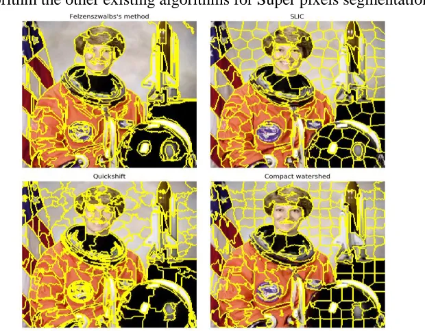
SLIC is better algorithm the other existing algorithms for Super pixels segmentation of an image.
Figure 1.1: Output superpixel images of different algorithms
Http://www.ijetmr.com©International Journal of Engineering Technologies and Management Research [8] Table 1.1: Comparative analysis of superpixel algorithm with SLIC
GS NC SL WS MS TP QS SLIC
Under-segmentation error
0.23 0.22 0.24 0.2 0.19
Boundary recall 0.84 0.68 0.61 0.79 0.82
Segmentation speed
Segmentation accuracy (using on MSRC)
74.60% 75.90% 62.00% 75.10% 76.9%
Control over amount of superpixels
No Yes Yes No NO Yes No Yes
Control over superpixel compactness
No No No No No No No Yes
Supervoxel extension No No No Yes No No No Yes
Complexity O(.)
Where N is number of Pixels
NlogN N3/2 N2logN NlogN N2 N dN2 N
7. Conclusion
Superpixels have become an essential tool to the vision community, and in this paper we provide the reader with an indepth performance analysis of modern superpixel techniques. We performed an empirical comparison of five state-of-theart algorithms, concentrating on their boundary adherence, segmentation speed, and performance. The kmeans clustering, based SLIC, has been shown to outperform existing superpixel methods in nearly every respect. Among the superpixel methods considered here, SLIC is clearly the best overall performer. It is the fastest method, segmenting a 2048×1536 image in 14.94s, and most memory efficient. It boasts excellent boundary adherence, outperforming all other methods in under-segmentation error, and is second only to GS04 in boundary recall by a small margin (by adjusting m, it ranks first). When used for segmentation, SLIC showed the best boost in performance on the MSRC and PASCAL datasets. SLIC is simple to use, its sole parameter being the number of desired superpixels, and it is one of the few methods to produce supervoxels. Finally, among existing methods, SLIC is unique in its ability to control the trade-off between superpixel compactness and boundary adherence if desired, through m.
References
[1] X. Ren and J. Malik, “Learning a classification model for segmentation,” in Proc. IEEE Conf.
International Conference on Computer Vision (ICCV), pp. 10-17, 2003.
[2] Pedro Felzenszwalb and Daniel Huttenlocher.Efficient graph-based image segmentation.
International Journal of Computer Vision (IJCV), 59(2):167–181, September 2004.
[3] Jianbo Shi and Jitendra Malik.Normalized cuts and image segmentation.IEEE Transactions on
Pattern Analysis and Machine Intelligence(PAMI), 22(8):888–905, Aug 2000.
[4] Y. Boykov and M. Jolly.Interactive Graph Cuts for Optimal Boundary & Region Segmentation
of Objects in N-D Images.In International Conference on Computer Vision (ICCV), 2001.
[5] A. Lucchi, K. Smith, R. Achanta, V. Lepetit, and P. Fua. A fully automated approach to
segmentation of irregularly shaped cellular structures in em images. International Conference
Http://www.ijetmr.com©International Journal of Engineering Technologies and Management Research [9]
[6] S. Gould, J. Rodgers, D. Cohen, G. Elidan, and D. Koller, “Multiclass segmentation with
relative location prior,” IJCV, 2008.
[7] J. M. Gonfaus, X. Boix, J. Van de Weijer, A. D. Bagdanov, J. Serrat, and J. Gonzalez,
“Harmony potentials for joint classification and segmentation,” in CVPR, 2010
[8] R. Achanta, A. Shaji, K. Smith, A. Lucchi, P. Fua, and S. Susstrunk, “Slicsuperpixels compared
to state-of-the-art superpixel methods,” TPAMI, 2012.
[9] S. Gould, J. Rodgers, D. Cohen, G. Elidan, and D. Koller, “Multiclass segmentation with
relative location prior,” IJCV, 2008.
[10] J. Shotton, J. Winn, C. Rother, and A. Criminisi, “Textonboost: Joint appearance, shape and
context modeling for multi-class object
recognition and segmentation,” in ECCV, 2006.
[11] T. Malisiewicz and A. A. Efros, “Improving spatial support for objects via multiple
segmentations,” in BMVC, 2007
[12] Y. Qin, H. Lu, Y. Xu, and H. Wang, “Saliency detection via cellular automata,” in CVPR, 2015
[13] Q. Yang, “A non-local cost aggregation method for stereo matching,” in CVPR, 2012
[14] X. Mei, X. Sun, W. Dong, H. Wang, and X. Zhang, “Segment-tree based cost aggregation for
stereo matching,” in CVPR, 201
[15] J. Shi, J. Malik. Normalized cuts and image segmentation. Transactions on Pattern Analysis and
Machine Intelligence, 22(8):888–905, 2000
[16] X. Ren, J. Malik. Learning a classification model for segmentation. International Conference on Computer Vision, pages 10–17, 2003.
[17] Alastair Moore, Simon Prince, Jonathan Warrell, Umar Mohammed, and Graham
Jones.Superpixel Lattices.IEEE Computer Vision and PatternRecognition (CVPR), 2008.
[18] ShaiAvidan and Ariel Shamir. Seam carving for content-aware image resizing. ACM
Transactions on Graphics (SIGGRAPH), 26(3), 2007
[19] A. Vedaldi, S. Soatto. Quick shift and kernel methods for mode seeking. European Conference
on Computer Vision, pages 705–718, 2008.
[20] A. Levinshtein, A. Stere, K. N. Kutulakos, D. J. Fleet, S. J. Dickinson, K. Siddiqi. TurboPixels:
Fast superpixels using geometric flows. Transactions on Pattern Analysis and Machine Intelligence, 31(12):2290–2297, 2009
[21] Luc Vincent and Pierre Soille. Watersheds in digital spaces: An efficient algorithm based on
immersion simulations. IEEE Transactions onPattern Analalysis and Machine Intelligence,
13(6):583–598, 1991.
[22] D. Comaniciu and P. Meer. Mean shift: a robust approach toward feature space analysis. IEEE
Transactions on Pattern Analysis and MachineIntelligence, 24(5):603–619, May 2002
[23] J. Shen, Y. Du, W. Wang, and X. Li, “Lazy random walks for superpixel segmentation,” IEEE
Trans. Image Process., vol. 23, no. 4, pp. 1451–1462, Apr. 2014
[24] O. Veksler, Y. Boykov, and P. Mehrani, “Superpixels and supervoxels in an energy
optimization framework,” in Proc. ECCV, 2010, pp. 211–224.
[25] D. Martin, C. Fowlkes, D. Tal, and J. Malik, “A database of human segmented natural images
and its application to evaluating segmentation algorithms and measuring ecological statistics,” in Proc. IEEE Int. Conf.Comput. Vis., vol. 2. Jul. 2001, pp. 416–423.
[26] Achanta, Radhakrishna, et al. "SLIC superpixels compared to state-of-the-art superpixel methods." IEEE transactions on pattern analysis and machine intelligence 34.11 (2012): 2274-2282.
*Corresponding author.