Simulation of Singular Fourth- Order Partial Differential
Equations Using the Fourier Transform Combined With
Variational Iteration Method
S. S. Nourazar
1*, H. Tamim
2, S. Khalili
3, A. Mohammadzadeh
41- Associate Professor, Department of Mechanical Engineering, Amirkabir University of Technology, Tehran, Iran 2- MSc Student, Department of Mechanical Engineering, Amirkabir University of Technology, Tehran, Iran 3- MSc Student, Department of Mechanical Engineering, Amirkabir University of Technology, Tehran, Iran
4- MSc Student, Tehran university alumnus in mechanical engineering, Tehran, Iran
ABSTRACT
In this paper, we present a comparative study between the modified variational iteration method (MVIM) and a hybrid of Fourier transform and variational iteration method (FTVIM). The study outlines the efficiency and convergence of the two methods. The analysis is illustrated by investigating four singular partial differential equations with variable coefficients. The solution of singular partial differential equations usually needs a coordinate transformation in order to discard the singularity of the partial differential equation. Most often this transformation is not applicable and even does not exist. Therefore in this case the solution for the singular partial differential equation does not exist. In the present study the results of simulation for the singular partial differential equations with variable coefficients using the Fourier transform variational iteration method are compared with the results of simulation using the modified variational iteration method. The comparison shows that the effectiveness and accuracy of Fourier transform variational iteration method is more than that of the modified variational iteration method for the simulation of singular partial differential equations.
KEYWORDS
Fourier Transformation Modified Variational Iteration Method, Hybrid of Fourier Transform, Variational Iteration Method, Singular Partial Differential Equations With Variable Coefficients.
٭Corresponding Author, Email: [email protected] Amirkabir University of Technology
(Tehran Polytechnic) Vol. 45, No.1, Spring 2013, pp. 27- 45
Amirkabir International Journal of Science & Research (Modeling, Identification, Simulation & Control)
1- INTRODUCTION
This paper outlines a reliable comparison between two powerful methods that were recently developed. The first is a hybrid of Fourier transform and variational iteration method (FTVIM) developed by S.S. Nourazar et al in [1]. The second is the modified variational iteration method (MVIM) developed by M. A. Noor et al in [2].
This paper is devoted to the study of the singular fourth - order parabolic partial differential equation with variable coefficient. It is well known in the literature that a wide class of problems arising in mathematics, physics and astrophysics and engineering sciences may be distinctively formulated as singular initial and boundary value problems. Singular fourth order parabolic partial differential equations govern the transverse vibrations of a homogeneous beam. Such types of equation arise in the mathematical modeling of viscoelastic and inelastic flows, deformation of beams and plate deflection theory, see [4 - 10]. The studies of such problems have attracted the attention of many mathematicians and physicists. So finding a method with less amount of computational work in comparison with the previous methods may be useful. The study of fourth - order partial differential equations with variable coefficients are performed by solving the vibration equation of beam and shafts using the second - order finite difference method [4, 5]. However in their results the convergence of the solution with mesh refinement failed and therefore the accuracy of the results was limited to a certain amount of refined mesh. Wazwaz [6, 8, 9] studied the behavior of the fourth - order partial differential equations with variable coefficients. The application of such equations encounters in the study of deformation of beams and plates as well as the flow of viscoelastic and elastic fluids. Wazwaz [6, 8, 9] solved the governing equations using the semi - analytical method such as the Adomian decomposition method. However in the Adomian decomposition method the boundary conditions of the governing equation were totally ignored. This may cause an inaccurate results as well as incorporating enormous amounts of terms in series solution. In the present study we intend to use the FTVIM developed by Nourazar et al [1] to solve the singular fourth - order
partial differential equations with variable coefficients that may arise in the study of the vibration of beams and plates as well as the flow of viscoelastic and elastic (Newtonian) fluid. These equations are solved by using the modified He’s variational iteration method (MVIM) [2]. First, a coordinate transformation is used to resolve the singularity problem and then the MVIM [2] is applied to solve the governing equations. However, the advantage of the FTVIM is that there is no need to find a coordinate transformation to get rid of the singularity problem. We show the effectiveness of the FTVIM by solving four singular fourth - order parabolic differential equations with variable coefficients as case studies. The first case study problem is the vibration of an elastic beam with variable material properties along the axis of beam. In the second case study we solve the vibration of a thin two dimensional elastic plate with variable material properties along the two dimensions (x, y). In the third case study we solve the governing equation of a three dimensional vibrating plate with external sinusoidal forcing function. In the fourth case study we consider the vibration of an elastic beam with a sinusoidal variable property along the beam axis.
2- NUMERICAL APPLICATION
In this section, we apply the FTVIM proposed by S.S. Nourazar et al in [1] for solving the fourth order parabolic partial differential equations. For using FTVIM we construct a correction functional by using the Lagrange multipliers that calculated optimally via variational theory. And finally we can approximate the exact solutions. For the sake of comparison, we take the same examples as used in [2] and the numerical results are very encouraging and conclusive.
●EXAMPLE 1
Consider the following singular fourth parabolic partial differential
2 1 4 4 1
0 1 , 0
2 120 4 2
u x u x t
x
t x
∂ + + ∂ = < < >
∂ ∂ (1)
With initial conditions:
1
( ,0) 0 1
2
u x = < <x (2)
5 1
( ,0) 1 1
120 2
x
u x x
t
∂ = + < <
Amirkabir International Journal of Science& Research (Modeling, Identification, Simulation & Control)
(AIJ-MISC)
Simulation of singular fourth- order partial differential equations using the Fourier transform combined with variational iteration method
First we take Fourier transform from equation (1) and immediately construct a correction functional as is done in reference [3]. Here û denotes the Fourier transform of u. Now for using FTVIM we construct a correction functional as[3]:
4
2 1 4 1 4
� 1( , ) �( , ) ( ) 2 �( , ) 4 4 4
120 0
t un
un t un t un F un F d
x x x
ω ω λ ξ ω ξ ξ
ξ ω
∂ ∂ ∂ ∂
= +∫ + +
+ ∂ ∂ ∂ ∂
ûn ûn ûn
(4) For detailed derivation of constructing the correction functional (Eq. (4)) one may refer to Wazwaz [3]. By using the variational principle and integrating by parts we may obtain the following. Integrating by parts and take first variation, we getλ ξ( )= −ξ t as follows:
4
2 1 4 1 4
� 1( , ) �( , ) ( ) 2�( , ) 4 4 4
120 0
t un
un t un t un F un F d
x x x
δ ω δ ω δ λ ξ ω ξ ξ
ξ ω
∂ ∂ ∂ ∂
⇒ + = + ∫ + +
∂ ∂ ∂ ∂
ûn
ûn ûn ûnûn
(5)
2
� 1( , ) �( , ) ( ) 2 �( , ) 0
t
un t un t un d
δ ω δ ω δ λ ξ ω ξ ξ
ξ
∂
⇒ + = + ∫
∂
ûn ûn ûn (6)
� 1 � ( ) � ( )� ( )�
un un un un u dn
δ δ δ λ ξ λ ξ λ ξ ξ
ξ
∂ ′ ′′
⇒ + = + ∂ − + ∫
ûn ûn ûn ûn ûn (7)
� 1 1 ( ) � ( ) � ( ) �
0 t
un un un u dn
δ λ ξ δ δλ ξ λ ξ δ ξ
ξ
∂
′ ′′
⇒ ûn + = − ûn + ∂ ûn +∫ ûn (8)
1 ( ) 0
( ) 0 ( )
( ) 0
t
t t
t
λ ξ ξ
λ ξ ξ λ ξ ξ
λ ξ ξ
− ′ =
=
⇒ = = ⇒ = −
′′
= =
(9)
Assuming u0(x, t), using the same method as used in [3], and substituting for the value of λ ξ( )= −ξ t, into Eq.(4)
the successive approximation uûn�n+1( , )ωt are obtained as follows: 4
2 1 4 1 4 0
�1( , ) �0( , ) ( ) 2 �0( , ) 4 0 4 4
120 0
t u
u t u t t u F u F d
x x x
ω ω ξ ω ξ ξ
ξ ω
∂ ∂ ∂ ∂
= +∫ − + +
∂ ∂ ∂ ∂
û1 û0 û0
(10)
(11)
(12)
4
2 1 4 1 4
� 1( , ) �( , ) ( ) 2 �( , ) 4 4 4
120 0
t un
un t un t t un F un F d
x x x
ω ω ξ ω ξ ξ
ξ ω
∂ ∂ ∂ ∂
⇒ + = +∫ − + +
∂ ∂ ∂ ∂
ûn ûn ûn
(13) For obtaining u x t1( , ) first we calculate followings:
5 ( , ) 1
0 120x
u x t = + t
(14)
Eq. (14) is obtained by integrating the Neumann initial condition (Eq. (3)) and considering as u x t0( , ).
( )
(
5, 6 120 120 ( ) 6 120 5)
1
�( , )0 6
120
I Dirac Dirac I
u ωt π ω ω π ω ω ω t
ω
− + −
=
û0 (15)
4 5
1 1
4 120
x t t
x x
∂ + =
4 5 1
4 120
x t xt x
∂ + =
∂ (17)
4
1 ( )
0 4
I
F u Dirac t
x x π ω ω
∂
= −
∂
(18)
(19)
(20)
(21)
Using the Maple package the inverse Fourier transform, u x t1( , )is:
5 3
( , ) 1
1 120x t6
u x t = + t−
(22)
Here, we are taking the inverse Fourier transform from equation (21) using the Maple package. After some simple manipulations we get Eq. (22)
For calculating u2(x,t) , we use the correction functional of Eq. (4) using the value of û1(ɷ,t) and taking the inverse Fourier transform as:
û1(ω, ξ) = ( I π Dirac(5, ω) ω6 - 120 + 120 π Dirac (ω) ω6 - ω6
ξ2
2 1
120 120 I ω ×(-ξ)
5
(23)
4 3
1 ( )
1
4 6
I t
F u Dirac t
x x π ω ω
∂
= − −
∂
Amirkabir International Journal of Science& Research (Modeling, Identification, Simulation & Control)
(AIJ-MISC)
Simulation of singular fourth- order partial differential equations using the Fourier transform combined with variational iteration method
8I (π Dirac (4, ω) ω2 + 6π Dirac (3,ω) ω + 6π Dirac (2,ω)) ω3
36I ( π Dirac (3, ω) ω2 + 4π Dirac (2,ω) ω + 2π Dirac (1,ω)) ω4
+
F u1 = I(πDirac(5,ω) ω
2 + 8 πDirac (4,ω) ω -12πDirac(3,ω))
ω2 ω4 4 4 x4
(
)
(
)
(
)
(
)
4 4 1 4 42
2 ) (4, 8 ) (3, 12 ) (4, 8 ) (5,
6 (3, ) 6 (2, ) 2 3 2
2 ) (2, 96 ) (1, 2 ) (2, 4 ) (3, 36
2 (1, ) 12 4 5 I Dirac Dirac Dirac I Dirac Dirac Dirac F u x I Dirac Dirac Dirac I Dirac Dirac π ωω π ωω π ω π ωω π ωω π ω ω ω ω π ωω π ωω π ω π ωω π ωω ω ω + + + + ∂ ∂ = − ∂ ∂ + + + + − +
(
)
2 ) (1, 0 3 6 6 I Dirac It t ωω π
ω + − ×
96I(πDirac(2,ω)ω2 + 2π Dirac (1,ω)ω) 120I(πDirac(1,ω)ω2 + I)
ω5 ω6
+ +
(
) (
)
(
) (
)
4 4 1 4 4 2 2(5, ) 8 (4, ) 12 (3, ) 8 (4, ) 6 (3, ) 6 (2, )
2 3
2 2
36 (3, ) 4 (2, ) 2 (1, ) 96 (2, ) 2 (1, ) 12
4 5
I Dirac Dirac Dirac I Dirac Dirac Dirac
F u
x
I Dirac Dirac Dirac I Dirac Dirac
π ω ω π ω ω π ω π ω ω π ω ω π ω ω ω ω π ω ω π ω ω π ω π ω ω π ω ω ω ω + + + + ∂ ∂ = − ∂ ∂ + + + + − +
(
)
20 (1, ) 3
6 6
I Dirac I t
t π ω ω ω + × −
(
) (
)
(
) (
)
4 4 1 4 4 2 2(5, ) 8 (4, ) 12 (3, ) 8 (4, ) 6 (3, ) 6 (2, )
2 3
2 2
36 (3, ) 4 (2, ) 2 (1, ) 96 (2, ) 2 (1, ) 12
4 5
I Dirac Dirac Dirac I Dirac Dirac Dirac
F u
x
I Dirac Dirac Dirac I Dirac Dirac
π ω ω π ω ω π ω π ω ω π ω ω π ω ω ω ω π ω ω π ω ω π ω π ω ω π ω ω ω ω + + + + ∂ ∂ = − ∂ ∂ + + + + − +
(
)
20 (1, ) 3
6 6
I Dirac I t
t π ω ω ω + × −
(
)
(
)
(
)
(
)
4 4 1 4 42
2 ) (4, 8 ) (3, 12 ) (4, 8 ) (5,
6 (3, ) 6 (2, ) 2 3 2
2 ) (2, 96 ) (1, 2 ) (2, 4 ) (3, 36
2 (1, ) 12 4 5 I Dirac Dirac Dirac I Dirac Dirac Dirac F u x I Dirac Dirac Dirac I Dirac Dirac π ωω π ωω π ω π ωω π ωω π ω ω ω ω π ωω π ωω π ω π ωω π ωω ω ω + + + + ∂ ∂ = − ∂ ∂ + + + + − +
(
)
2 ) (1, 0 3 6 6 I Dirac It t ωω π
ω + − × t - t3 6
× (25)
Using correction functional and the Maple package, the inverse Fourier transform, u x t2( , )is:
5 3 5
( , ) 1
2 120x t6 120t
u x t = + × −t +
(26)
Here, we are using the correction functional of Eq. (4) and taking the inverse Fourier transform one gets Eq. (26). For u x t3( , ):
( )
(
5, 6 120 120 ( ) 6 120 5)
2 1 1 3
�( , )2
2 120 6 6
I Dirac Dirac I
u ωt π ω ω π ω ω ω ξ ξ
ξ ω
− + −
∂ = × − +
∂ û2 (27)
4 3 5
1 ( )
2
4 6 120
I t t
F u Dirac t
x x π ω ω
∂
= − × − +
∂
(28)
(29)
Using correction functional and the Maple package the Fourier transform and inverse Fourier transform, u3(x,t) is:
5 3 5 7
( , ) 1
3 120x t6 120 5040t t u x t = + t− + −
(30)
And so on. The Taylor series expansion for sin (t) is written as:
( )
(
)
0
(2 1) 3 5 7
1 sin( )
2 1 ! 6 120 5040
n
i
it i t t t
t t i = + − = = − + − + +
∑
(31)And:
( , ) lim n
u x t un
→∞
= (32)
By substituting Eq (31) into Eq (30) thus Eq (30) can ultimately be reduced to:
5
( , ) lim 1 sin( )
120 n
x
u x t un t
→∞
= = +
(33)
Which, it is the exact solution.
● EXAMPLE 2
Consider the following singular fourth parabolic partial differential equation in two space variables:
2 1 4 4 1 4 4
2 2 0
2 2 6! 4 2 6! 4
u x u y u
t x x y y
∂ + + ∂ + + ∂ =
With initial conditions:
6 6
( , ,0) 0, ( , ,0) 2
6! 6!
u x y
u x y x y
t
∂
= = + +
∂ (35)
Now using FTVIM we construct a correction functional as:
2� ( , , ) 1 4 4 ( , , ) 1 4 4 ( , , )
� 1( , , ) �( , , ) ( ) 2 2 2 4 2 2 4
6! 6!
0
t un y x u x yn y u x yn
un y t un y t F F d
x x y y
ω ξ ξ ξ
ω ω λ ξ ξ
ξ
∂ ∂ ∂
= +∫ + + + +
+ ∂ ∂ ∂
ûn ûn ûn
(36) Integrating by parts and taking the first variation, we get λ ξ
( )
= −ξ tas follows:2� ( , , ) 1 4 4 ( , , ) 1 4 4 ( , , )
� 1( , , ) �( , , ) ( ) 2 2 2 4 2 2 4
6! 6!
0
t un y x u x yn y u x yn
un y t un y t F F d
x x y y
ω ξ ξ ξ
δ ω δ ω δ λ ξ ξ
ξ
∂ ∂ ∂
⇒ + = + ∫ + + + +
∂ ∂ ∂
ûn ûn ûn (37)
2 �( , , ) � 1( , , ) �( , , ) ( ) 2
0
t un y
un y t un y t ω ξ d
δ ω δ ω δ λ ξ ξ
ξ
∂
⇒ + = + ∫
∂
ûn ûn ûn (38)
�
� 1 � ( ) un ( )� ( )�
un un un u dn
δ δ δ λ ξ λ ξ λ ξ ξ
ξ ∂
′ ′′
⇒ + = + ∂ − + ∫
ûn ûn ûn ûn ûn (39)
�
� 1 1 ( ) � ( ) ( )�
0 t un
un un u dn
δ λ ξ δ δλ ξ λ ξ ξ
ξ
∂
′ ′′
⇒ ûn+ = − ûn + ∂ûn +∫ ûn (40)
1 λ ξ′( )ξ t 0 λ ξ( )ξ t 0 λ ξ′′( )ξ t 0 λ ξ( ) ξ t
⇒ − = = = = = = ⇒ = − (41)
Assuming 0( , , ) 2 6 6 6! 6!
x y
u x y t = + + t
, using the same method as used in [3], and substituting for the value of λ ξ
( )
= −ξ tinto Eq. (36) the successive approximation ûn +1 (ɷ,y,t)are obtained as follows:
(42)
(43)
(44)
(45)
For obtaining u x y t1( , , ), first we calculate followings:
4 6 6 1 2
2
4 6! 6! 2
x y t x t
x
∂ + + =
∂ (46)
4 6 6 1 2
2
4 6! 6! 2
x y t y t y
∂ + + =
∂ (47)
4 4
1 2 2 1 2 1 1 6
2 2
2 6! 720 720
x x
x t x t t tx
x x
× + = + = +
Amirkabir International Journal of Science& Research (Modeling, Identification, Simulation & Control)
(AIJ-MISC)
Simulation of singular fourth- order partial differential equations using the Fourier transform combined with variational iteration method
4 4
1 2 2 1 2 1 1 6
2 2
2 6! 720 720
y y
y t y t t ty
y y
× + = + = +
(49)
6 6 1 1440 ( ) 7 ( ) 7 6 (6, ) 7 720 1440 6 6 6
2 7
6! 6! 720
x y Dirac Dirac y Dirac I I I y
F t π ω ω π ω ω π ω ω ω ω t
ω
+ − + − −
+ + =
(50)
(51)
(
)
1 6 1 ( ) 720 6
720 360
F t + ty = πDirac ω +y t
(52)
(
)
(
)
7
7 7 6 7 6 6 6
1 1440 ( ) ( ) (6, ) 720 1440
�( , , )1 7
720 0 720
7 7 6
(6, ) 720 ( ) 720 720 720 6 ( )
360
t
Dirac Dirac y Dirac I I I y
u y t t t
Dirac Dirac I I y Dirac d
π ω ω π ω ω π ω ω ω ω ξ
ω ξ
ω
π ω ω π ω ω ω ξ π ω ξ
ω
+ − + − −
= +∫ −
− + + − + +
û1(
(
)
(
)
7
7 7 6 7 6 6 6
1 1440 ( ) ( ) (6, ) 720 1440
�( , , )1 7
720 0 720
7 7 6
(6, ) 720 ( ) 720 720 720 6 ( )
360
t
Dirac Dirac y Dirac I I I y
u y t t t
Dirac Dirac I I y Dirac d
π ω ω π ω ω π ω ω ω ω ξ
ω ξ
ω
π ω ω π ω ω ω ξ π ω ξ
ω
+ − + − −
= +∫ −
− + + − + +
(53)
Using the Maple package, the inverse Fourier transform, u x y t1( , , )is:
(
)(
)
3 6 61 2 6 6
( , , ) 6 1440 2
1 4320 t6 x6! y6!
u x y t = − t − +t +x +y =t− + +
(54)
For u x y t2( , , )
(
)
4 4 3 6 6 1 3 2
( , , ) 2
1
4 4 6 6! 6! 2 6
t x y t
u x y t t t x
x x
∂ = ∂ − + + = −
∂ ∂ (55)
(
)
4 4 3 6 6 1 3 2
( , , ) 2
1
4 4 6 6! 6! 2 6
t x y t
u x y t t t y
y y
∂ = ∂ − + + = −
∂ ∂ (56)
(57)
(58) Using correction functional and the Maple package, the Fourier transform and inverse Fourier transform, u2(x, y, t) is:
(59)
For u x y t3( , , )
(60)
(61)
(63)
Using correction functional and the Maple package, the Fourier transform and inverse Fourier transform, u3(x, y, t) is:
(64)
And so on. The Taylor series expansion for sin(t)is written as:
(65)
And
( , , ) lim
u x y t un
n
=
→ ∞ (66)
By substituting Eq. (64) and Eq. (65) into Eq. (66) thus Eq. (64) can ultimately be reduced to:
6 6
( , , ) lim 2 sin( )
6! 6!
x y
u x y t un t
n
= = + + ×
→ ∞ (67)
Which, it is the exact solution of Eq. (34).
● EXAMPLE 3
Considering the following three dimensional non - homogenous singular partial differential equation, we solve this equation with FTVIM.
( )
2 4 4 4
2 4 4 4 5 5 5
1 1 1 1 1 1 cos
4! 4! 4!
u u u u x y z t
t z x x y y z y z x x y z
∂ − ×∂ + ×∂ + ×∂ = − + + + + +
∂ ∂ ∂ ∂ (68)
With initial condition:
( , , ,0) x y z
u x y z
y z x
= + + (69)
Now we construct a correction functional as:
( )
4 4
4 4
4
1 0 4
2
5 5 5 2
1 ( , , , ) 1 ( , , , )
4! 4!
1 ( , , , )
� ( , , , ) �( , , , ) ( )
4!
1 1 1 cos ( , , , )
n n
t n
n n
n
u y z t u y z t
z x x y
u y z t
u y z t u y z t F d
y z
x y z u y z t
y z x x y z
ω ω
ω
ω ω λ ξ ξ
ω ξ
ξ
+
×∂ + ×∂
∂ ∂
−
∂
+ ×
= + × ∂
∂
+ + + + + + +
∂
∫
ûn+1 ûn+1
(70)
Integrating by parts and taking the first variation, we get λ ξ( )= −ξ t as follows:
( )
4 4 4
4 4 4
1 0 2
5 5 5 2
1 1 1
4! 4! 4!
� � ( )
1 1 1 cos
n n n
t
n n
n
u u u
z x x y y z
u u F d
x y z u
y z x x y z
δ δ δ λ ξ ξ
ξ ξ +
− ×∂ + ×∂ + ×∂
∂ ∂ ∂
⇒ = + ×
∂
+ + + + + + +
∂
∫
ûn+1 ûn (71)
( )
4 4 4
4 4 4
2
1 0 2 0
5 5 5
1 1 1
4! 4! 4!
� � ( ) ( )
1 1 1 cos
n n n
t n t
n n
u u u
z x x y y z
u
u u F d F d
x y z
y z x x y z
δ δ δ λ ξ ξ δ λ ξ ξ
ξ
ξ
+
− ×∂ + ×∂ + ×∂
∂ ∂ ∂
∂
⇒ = + × ∂ + ×
+ + + + + +
∫
∫
Amirkabir International Journal of Science& Research (Modeling, Identification, Simulation & Control)
(AIJ-MISC)
Simulation of singular fourth- order partial differential equations using the Fourier transform combined with variational iteration method
2
1 0 2
�
� � t ( ) n
n n u
u u d
δ δ δ λ ξ ξ
ξ
+
∂
⇒ = + ×
∂
∫
ûn+1 ûn
ûn
(73)
1 0
�
� � ( ) n ( )� t ( )�
n n u n n
u u u u d
δ δ δ λ ξ λ ξ λ ξ ξ
ξ
+
∂ ′ ′′
⇒ = + × − +
∂
∫
ûn
ûn
ûn ûn d
ûn+1 (74)
[ ]
1 � 0
� 1 ( ) � ( ) n t ( )�
n n u n
u u u d
δ λ ξ δ δ λ ξ δ λ ξ ξ
ξ
+
∂
′ ′′
⇒ = − + × +
∂
∫
ûn+1 ûn
ûn
ûn d (75)
1 ( ) 0
( ) 0 ( )
( ) 0
t
t
t
t ξ
ξ
ξ
λ ξ
λ ξ λ ξ ξ
λ ξ
= =
=
− ′ =
⇒ = ⇒ = −
′′ =
(76)
Assuming u0 (x, y, z, t) = u (x, y, z, 0), using the same method as used in [3], and substituting for the value of
( ) t
λ ξ = −ξ , and using Eq. (70) the successive approximation ûn+1 (ɷ, y, z, t) are obtained as follows:
(77)
(78)
(79)
(80)
For obtaining û1 (ɷ, y, z, t), first we calculate following terms:
( )
2
0
2u x y z t, , , 0 t
∂ =
∂ ( )
4
0
4 5
24
, , , z
u x y z t
x x
∂ =
∂ ( )
4
0
4 5
24
, , , x
u x y z t
y y
∂ =
∂
( )
4
0
4 5
24
, , , y
u x y z t
z z
∂ =
∂
4
0
4 5
1 ( , , , ) 1
4!z x u ω y z t x
∂
× =
∂ (81)
(82) Using the Maple package, the inverse Fourier Transform, u x y z t1( , , , ) is:
( ) 2 ( ) ( ) 2 2 ( ) ( ) ( ) ( )
1 5 5 5 5 5 5 5 5 5
cos cos cos cos cos cos
1 1 1 1 1 1
, , ,
2 2 2
t x t t t y t z t
t t t
u x y z t
x x x z y y z y z z y x
= − + − + + + + + + − + 1( ) ( ) 2
5 5 5 5 5 5 5 5 5
1 1 1 1 1 1 1 1 1
, , , cos
2
x y z t
u x y z t t
y z x x y z x y z x y z
→ = + + + + + − + + + + +
( ) ( ) 2
1 5 5 5 5 5 5
1 1 1 1 1 1
, , , cos 1
2
x y z t
u x y z t t
y z x x y z x y z
→ = + + + + + − + + −
( ) ( ) 2
1 5 5 5 5 5 5 5 5 5
1 1 1 1 1 1 1 1 1
, , , cos
2
x y z t
u x y z t t
y z x x y z x y z x y z
→ = + + + + + − + + + + +
(83)
(
)
( )
21 5 5 5 5 5 5
1 1 1 1 1 1
, , , cos 1
2
x y z t
u x y z t t
y z x x y z x y z
= + + + + + − + + −
(
)
( )
( )
2 1
2 5 5 5 5 5 5
1 1 1 1 1 1
, , , cos cos x y z
u x y z t t t
t x y z x y z y z x
∂ = + + − + + − + +
∂
(
)
( )
( )
2 1
2 5 5 5 5 5 5
1 1 1 1 1 1
, , , cos cos x y z
u x y z t t t
t x y z x y z y z x
∂ = + + − + + − + +
∂ (84)
(
)
( )
( )
4 2
1
4 5 9 9 9
24 cos 840 1680cos 1680
, , , z t t t
u x y z t
x x x x x
∂
= + + −
∂
(
)
( )
( )
4 2
1
4 5 9 9 9
24 cos 840 1680cos 1680
, , , x t t t
u x y z t
y y y y y
∂ = + + −
∂ (85)
(
)
( )
( )
4 2
1
4 5 9 9 9
24 cos 840 1680cos 1680
, , , y t t t
u x y z t
z z z z z
∂ = + + −
∂
(
)
( )
( )
4 2
1
4 5 9 9 9
cos 70cos
1 , , , 35 70
4!
t t t
u x y z t
z x x zx zx zx
∂ = + + −
∂
(
)
( )
( )
4 2
1
4 5 9 9 9
cos 70cos
1 , , , 35 70
4!
t t t
u x y z t
x y y xy xy xy
∂ = + + −
∂
(
)
( )
( )
4 2
1
4 5 9 9 9
cos 70cos
1 , , , 35 70
4!
t t t
u x y z t
y z z yz yz yz
∂ = + + −
∂ (86)
Using the Maple package, the inverse Fourier Transform, u x y z t2( , , , ) is:
(87) For u x y z t3( , , , )
Amirkabir International Journal of Science& Research (Modeling, Identification, Simulation & Control)
(AIJ-MISC)
Simulation of singular fourth- order partial differential equations using the Fourier transform combined with variational iteration method
(89)
(90)
Using the Maple package, the inverse Fourier Transform, u x y z t3( , , , ) is:
( )
(
)
(
)
(
)
(
)
(
)
(
)
12 8 4 12 8 4 12 8 4
4 12 8 4 12 8 4 12 8 4 2 12 8 4 12 8 4 12 8 4
6 11 13 13 11 11 13 11 13 13 11 11 13
3 13 13 13 2 11 13 13 11 11 13
5040cos 210 2520 3465 2494800 1 1 ( , , , ) 72 1247400
t z x y x y z y z x
t z x y x y z y z x t z x y x y z y z x
t z y z x y x z y z x y x
u x y z t
x y z t z y z x y x
+ + − + + + + + + + − + + = + + + −
(
)
(
)
( )(
)
(
)
( )(
)
4 11 13 13 11 11 13
12 8 4 12 8 4 12 8 4 11 13 13 11 11 13
6 12 8 4 12 8 4 12 8 4 13 12 14 14 13 12 12 14 13
103950
5040 2494800cos
7 72cos
t z y z x y x z x y x y z y z x t z y z x y x t z x y x y z y z x t z y x z y x z y x
+ + − + + + + + + + + + + +
(
)
( )(
)
( ) ( )(
)
2 4 6
12 8 4 12 8 4 12 8 4
2 4 6
11 13 13 11 11 13
3 13 13 13
13 12 14 14 13 12 12 14 13
5040 cos 1
2! 4! 6!
1 1
( , , , ) 2494800 cos 1
72 2! 4! 6!
72cos
t t t z x y x y z y z x t
t t t
u x y z t z y z x y x t
x y z
t z y x z y x z y x
+ + − + − + → = + + + − + − + + + + ( )
3 13 2 13 2 2 13 5 9 5 9 5 9 13 2 13 2 2 13
2 4 6
5 9 5 9 5 9
1 1 1 1 1 1 1 1 1
( , , , ) 34650 70 cos 34650
1 1 1
70 1
2! 4! 6!
x y z
u x y z t t
y z x z y y x z x z yx x zy y xz z y y x z x
t t t
z yx x zy y xz
→ = + + + + + + + + − + + + + + − + − ( )
3 13 2 13 2 2 13 5 9 5 9 5 9 13 2 13 2 2 13
2 4 6
5 9 5 9 5 9
1 1 1 1 1 1 1 1 1
( , , , ) 34650 70 cos 34650
1 1 1
70 1
2! 4! 6!
x y z
u x y z t t
y z x z y y x z x z yx x zy y xz z y y x z x
t t t
z yx x zy y xz
→ = + + + + + + + + − + + + + + − + −
(91)
And so on. The Taylor series expansion for cos(t) is written as:
( ) ( )( )2 2 4 6
0 1
cos 1
2 ! 2! 4! 6!
i i n
i
t t t t
t
i
=
−
=
∑
= − + − + (92)And
( , ) lim ( , )n n
u x t = →∞u x t (93)
By substituting Eq. (91) and Eq. (92) into Eq. (93) thus Eq. (91) can ultimately be reduced to Eq (94):
( )
13 2 13 2 2 13( )
3 13 2 13 2 2 13 5 9 5 9 5 9
5 9 5 9 5 9
1 1 1
34650
1 1 1 1 1 1
( , , , ) 34650 70 cos cos
1 1 1
70
z y y x z x
x y z
u x y z t t t
y z x z y y x z x z yx x zy y xz
z yx x zy y xz
+ + + = + + + + + + + + − + +
( ) 13 2 13 2 2 13 ( )
3 13 2 13 2 2 13 5 9 5 9 5 9
5 9 5 9 5 9
1 1 1
34650
1 1 1 1 1 1
( , , , ) 34650 70 cos cos
1 1 1
70
z y y x z x
x y z
u x y z t t t
y z x z y y x z x z yx x zy y xz
z yx x zy y xz
+ + + = + + + + + + + + − + +
(94)
Therefore, the exact solution is given as:
( )
( , ) lim ( , )n n x y z cos
u x t u x t t
y z x
→∞
= = + +
● EXAMPLE 4
Consider the following singular fourth parabolic partial differential.
2 4
2 sin( ) 1 4 0
u x u
t x x
∂ + − ∂ =
∂ ∂ (96)
With initial conditions:
( ,0) sin( ) 0 1
u x = −x x < <x (97)
[
]
( ,0) sin( ) 0 1
u x x x x
t
∂ = − − < <
∂ (98)
Now using FTVIM we construct a correction functional as:
(99) Integrating by parts and take first variation, we get λ ξ( )= −ξ t as follows:
2 4
1 0 2 4
�
� � ( ) 1
sin( )
t n n
n n u x u
u u F d
x x δ δ δ λ ξ ξ ξ + ∂ ∂ ⇒ = + ×∂ + − ∂
∫
ûn+1 ûn ûn
(100)
2
1 0 2
�
� � t ( ) n
n n u
u u d
δ δ δ λ ξ ξ ξ + ∂ ⇒ = + × ∂
∫
ûn+1 ûn ûn
(101)
1 � 0
� � ( ) n ( ) � t ( ) �
n n u n n
u u u u d
δ δ δ λ ξ λ ξ λ ξ ξ ξ + ∂ ′ ′′ ⇒ = + × − × + × ∂
∫
ûn+1 ûn
ûn û
n ûn d (102)
1 � 0
� � ( ) n ( ) � t ( ) �
n n u n n
u u u u d
δ δ δ λ ξ λ ξ λ ξ ξ ξ + ∂ ′ ′′ ⇒ = + × − × + × ∂
∫
ûn+1 ûn
ûn û
n ûn d
ûn ûn d (103)
1 ( ) 0
( ) 0 ( )
( ) 0
t t t t ξ ξ ξ λ ξ λ ξ λ ξ ξ λ ξ = = = − ′ = ⇒ = ⇒ = − ′′ = (104)
Assuming u0(x,t) = (x - sin (x)) (1-t), using the same method as used in [3], and substituting for the value of
( ) t
λ ξ = −ξ , into Eq. (99) the successive approximations, uû� ( , )nn+1+1ωt , are obtained as follows:
2 4
0 0
1 0 0 �( , )2 4
( , )
�( , ) �( , ) ( ) 1
sin( )
t u x u x
u t u t F d
x x ω ξ ξ ω ω λ ξ ξ ξ ∂ ∂ = + × ∂ + − ∂
∫
û0 ( û0 (
û1 ( (105)
2 4
1 1
2 1 0 2 4
�( , ) ( , )
�( , ) �( , ) ( ) 1
sin( )
t u x u x
u t u t F d
x x ω ξ ξ ω ω λ ξ ξ ξ ∂ ∂ = + × ∂ + − ∂
∫
û2 ( û1 ( û1 (
(106)
2 4
2 2
3 2 0 �( , )2 4
( , )
�( , ) �( , ) ( ) 1
sin( )
t u x u x
u t u t F d
x x ω ξ ξ ω ω λ ξ ξ ξ ∂ ∂ = + × ∂ + − ∂
∫
û3 ( û2 ( û2 ( (107)
2 4
1 0 2 4
�( , ) ( , )
� ( , ) �( , ) ( ) 1
sin( )
t n n
n n u x u x
u t u t F d
x x ω ξ ξ ω ω λ ξ ξ ξ + ∂ ∂ = + × ∂ + − ∂
∫
ûn+1 ûn
ûn
(108)
For obtaining û1 (ɷ, t) , first we calculate followings:
( ) ( )
4 0 4
1 sin( ) 1
sin( )
x u x x t
x x
− ∂ = − × −
∂
(109)
(
)
{
}
(
2 2)
(1, )
1 1 1
sin( ) (1 ) ( 1) ( 1) (1 )
2 2 ( )( 1)
I Dirac I
F x x t I Dirac I Dirac t
z ω π ω π ω π ω ω ω ω + − × − = + − − − − × − + −
Amirkabir International Journal of Science& Research (Modeling, Identification, Simulation & Control)
(AIJ-MISC)
Simulation of singular fourth- order partial differential equations using the Fourier transform combined with variational iteration method
Using Eq. (105) we obtain û1 (ɷ, t) as:
(111) Using the Maple package, the inverse Fourier Transform, u x t1( , ) is:
( ) 2 3
1( , ) sin( ) 1 2 6
t t
u x t = x− x × − + t −
(112)
For u x t2( , )
(
)
4 2 3
1 4
1 sin( ) 1
sin( ) 2 6
x u x x t t t
x x
∂
− = − × − + −
∂
(113)
Using correction functional and the Maple package, the inverse Fourier transform, u x t2( , ) is:
(
)
2 3 4 52( , ) sin( ) 1 2 6 24 120
t t t t
u x t = x − x × − + t − + −
(114)
For u x t3( , )
(
)
4 2 3 4 5
2 4
1 sin( ) 1
sin( ) 2 6 24 120
x u x x t t t t t
x x
− ∂ = − × − + − + −
∂
(115)
Using correction functional and the Maple package, the inverse Fourier transform, u x t3( , ) is:
( ) 2 3 4 5 6 7
3( , ) sin( ) 1 2 6 24 120 720 5040
t t t t t t
u x t = x − x × − + t − + − + −
(116)
And so on. The Taylor series expansion for e−t is written as:
( )
2 3 4 5 6 70
1 1 ...
! 2 6 24 120 720 5040
i i n t
i
t t t t t t t
e t
i
−
=
−
=
∑
= − + − + − + − + (117)And:
( , ) lim ( , )n n
u x t u x t
→∞
= (118)
By substituting Eq. (116) and Eq. (117) into Eq. (118) thus Eq. (116) can ultimately be reduced to:
( )
(
)
( , ) lim ( , ) sin t
n n
u x t u x t x x e−
→∞
= = − × (119)
Which, it is the exact solution of Eq. (96).
RESULTS
In the following tables and figures, we show the trend of convergence of u0 to u3 of the FTVIM and MVIM solution at three different locations and at three different times. The trend of rapid convergence of the FTVIM towards the exact solution is clearly shown. Using the new method, FTVIM, indicates that the amount of computational work is much less than that of the MVIM.
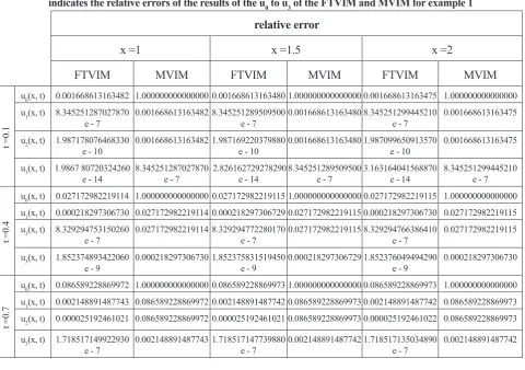
Table 1
indicates the relative errors of the results of the u0 to u3 of the FTVIM and MVIM for example 1 relative error
x =1 x =1.5 x =2
FTVIM MVIM FTVIM MVIM FTVIM MVIM
t =0.1
u0(x, t) 0.001668613163482 1.000000000000000 0.001668613163480 1.000000000000000 0.001668613163475 1.000000000000000 u1(x, t) 8.345251287027870
e - 7 0.001668613163482 8.345251289509500 e - 7 0.001668613163480 8.345251299445210 e - 7 0.001668613163475 u2(x, t) 1.987178076468330
e - 10 0.001668613163482 1.987169220379880 e - 10 0.001668613163480 1.987099650913570 e - 10 0.001668613163475 u3(x, t) 1.9867 80720324260
e - 14 8.345251287027870 e - 7 2.826162729278290 e - 14 8.345251289509500 e - 7 3.163164041568870 e - 14 8.345251299445210 e - 7
t =0.4
u0(x, t) 0.027172982219114 1.000000000000000 0.027172982219115 1.000000000000000 0.027172982219115 1.000000000000000 u1(x, t) 0.000218297306730 0.027172982219114 0.000218297306729 0.027172982219115 0.000218297306730 0.027172982219115 u2(x, t) 8.329294753150260
e - 7 0.027172982219114 8.329294772280170 e - 7 0.027172982219115 8.329294766386410 e - 7 0.027172982219115 u3(x, t) 1.852374893422060
e - 9 0.000218297306730 1.852375831519450 e - 9 0.000218297306729 1.852376049494290 e - 9 0.000218297306730
t =0.7
u0(x, t) 0.086589228869972 1.000000000000000 0.086589228869973 1.000000000000000 0.086589228869973 1.000000000000000 u1(x, t) 0.002148891487743 0.086589228869972 0.002148891487742 0.086589228869973 0.002148891487742 0.086589228869973 u2(x, t) 0.000025192461021 0.086589228869972 0.000025192461021 0.086589228869973 0.000025192461022 0.086589228869973 u3(x, t) 1.718517149922930
e - 7 0.002148891487743 1.718517147739880 e - 7 0.002148891487742 1.718517135034890 e - 7 0.002148891487742
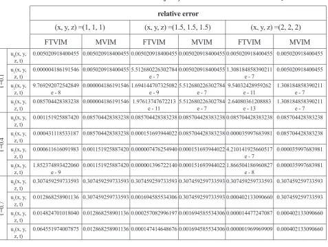
Table 2
indicates the relative errors of the results of the u0 to u3 of the FTVIM and MVIM for example 2 relative error
(x, y) =(1, 1) (x, y) =(1.5, 1.5) (x, y) =(2, 2)
FTVIM MVIM FTVIM MVIM FTVIM MVIM
t =0.1
u0(x, y, t) 0.001668613163476 1.000000000000000 0.001668613163479 1.000000000000000 0.001668613163476 1.000000000000000 u1(x, y, t) 8.345251280689990
e - 7 0.001668613163476 8.345251247541810 e - 7 0.001668613163479 8.345251299445220 e - 7 0.001668613163476 u2(x, y, t) 1.987154929508460
e - 10 0.001668613163476 1.987174944070330 e - 10 0.001668613163479 1.987121438012830 e - 10 0.001668613163476 u3(x, y, t) 3.000838008922480
e - 14 8.345251280689990 e - 7 2.465171745528260 e - 14 8.345251247541810 e - 7 3.219649113739740 e - 14 8.345251299445220 e - 7
t =0.4
u0(x, y, t) 0.027172982219114 1.000000000000000 0.027172982219114 1.000000000000000 0.027172982219114 1.000000000000000 u1(x, y, t) 0.000218297306730 0.027172982219114 0.000218297306730 0.027172982219114 0.000218297306729 0.027172982219114 u2(x, y, t) 8.329294758766400
e - 7 0.027172982219114 8.329294760610980 e - 7 0.027172982219114 8.329294761628440 e - 7 0.027172982219114 u3(x, y, t) 1.852375832984920
e - 9 0.000218297306730 1.852375593306180 e - 9 0.000218297306730 1.852375718504080 e - 9 0.000218297306729
t =0.7
u0(x, y, t) 0.086589228869979 1.000000000000000 0.086589228869971 1.000000000000000 0.086589228869976 1.000000000000000 u1(x, y, t) 0.002148891487736 0.086589228869979 0.002148891487741 0.086589228869971 0.002148891487742 0.086589228869976 u2(x, y, t) 0.000025192461024 0.086589228869979 0.000025192461017 0.086589228869971 0.000025192461023 0.086589228869976 u3(x, y, t) 1.718517101092090
Amirkabir International Journal of Science& Research (Modeling, Identification, Simulation & Control)
(AIJ-MISC)
Simulation of singular fourth- order partial differential equations using the Fourier transform combined with variational iteration method
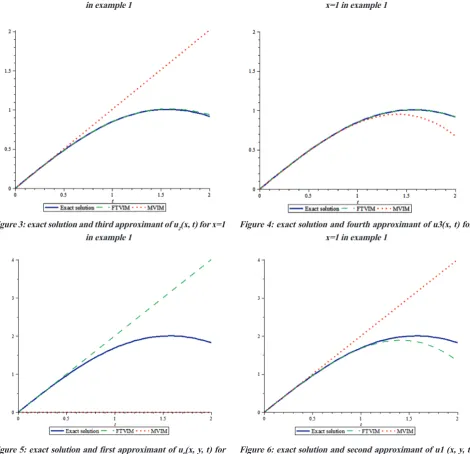
Table 3
indicates the relative errors of the results of the u0 to u3 of the FTVIM and MVIM for example 3 relative error
(x, y, z) =(1, 1, 1) (x, y, z) =(1.5, 1.5, 1.5) (x, y, z) =(2, 2, 2)
FTVIM MVIM FTVIM MVIM FTVIM MVIM
t =0.1
u0(x, y,
z, t) 0.005020918400455 0.005020918400455 0.005020918400455 0.005020918400455 0.005020918400455 0.005020918400455 u1(x, y,
z, t) 0.000004186191546 0.005020918400455 5.512680226302784 e - 7 0.005020918400455 1.308184858390211 e - 7 0.005020918400455 u2(x, y,
z, t) 9.769292072542849 e - 8 0.000004186191546 1.694144707325082 e - 9 5.512680226302784 e - 7 9.54032428959262 e - 11 1.308184858390211 e - 7 u3(x, y,
z, t) 0.085704428383238 0.000004186191546 1.97613747672213 e - 11 5.512680226302784 e - 7 2.64080361208883 e - 13 1.308184858390211 e - 7
t =0.4
u0(x, y,
z, t) 0.001151925887420 0.085704428383238 0.085704428383238 0.085704428383238 0.085704428383238 0.085704428383238 u1(x, y,
z, t) 0.000431118533187 0.085704428383238 0.000151693944022 0.085704428383238 0.000035997683981 0.085704428383238 u2(x, y,
z, t) 0.000611616091983 0.001151925887420 0.000007476254940 0.000151693944022 4.210141925660517 e - 7 0.000035997683981 u3(x, y,
z, t) 1.852374893422060 e - 9 0.001151925887420 0.000001396722140 0.000151693944022 1.866504186960827 e - 8 0.000035997683981
t =0.7
u0(x, y,
z, t) 0.307459259733593 0.307459259733593 0.307459259733593 0.307459259733593 0.307459259733593 0.307459259733593 u1(x, y,
z, t) 0.012868258901136 0.307459259733593 0.001694585534306 0.307459259733593 0.000402133090660 0.307459259733593 u2(x, y,
z, t) 0.014824701018040 0.012868258901136 0.000257082996197 0.001694585534306 0.000014477247087 0.000402133090660 u3(x, y,
z, t) 0.064551974007875 0.012868258901136 0.000147414648676 0.001694585534306 0.000001969969909 0.000402133090660
Table 4
indicates the relative errors obtained by the FTVIM, MVIM and the exact solution for example 4 relative error
x =1 x =1.5 x =2
FTVIM MVIM FTVIM MVIM FTVIM MVIM
t =0.1
u0(x, t) 0.005346173731916 0.105170918075647 0.005346173731918 0.105170918075647 0.005346173731917 0.105170918075647 u1(x, t) 0.000004514294554 0.005346173731916 0.000004514294552 0.005346173731918 0.000004514294551 0.005346173731917 u2(x, t) 1.513305096916960
e - 9 0.000004514294554 1.513301488251290 e - 9 0.000004514294552 1.513302398108410 e - 9 0.000004514294551 u3(x, t) 2.718850284455520
e - 13 1.513305096916960 e - 9 2.705167496830410 e - 13 1.513301488251290 e - 9 2.70541797905007 e - 13 1.513302398108410 e - 9
t =0.4
u0(x, t) 0.104905181415237 0.491824697641270 0.104905181415237 0.491824697641270 0.104905181415237 0.491824697641270 u1(x, t) 0.001472002378775 0.104905181415237 0.001472002378776 0.104905181415237 0.001472002378777 0.104905181415237 u2(x, t) 0.000008025075486 0.001472002378775 0.000008025075489 0.001472002378776 0.000008025075490 0.001472002378777
u3(x, t) 2.321196910569100
e - 8 0.000008025075486 2.321196991935650 e - 8 0.000008025075489 2.321196884804210 e - 8 0.000008025075490
t =0.7
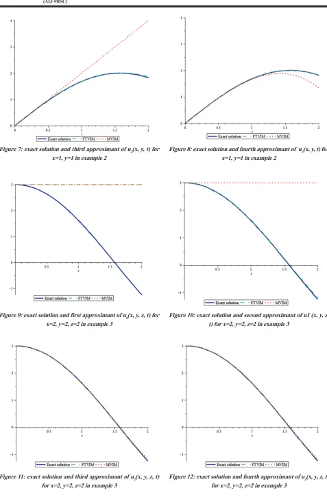
The efficiency and rapid convergence of FTVIM are shown in the following figures:
Figure 1: exact solution and first approximant of u0(x, t) for x=1
in example 1 Figure 2: exact solution and second approximant of u1 (x, t) for x=1 in example 1
Figure 3: exact solution and third approximant of u2(x, t) for x=1 in example 1
Figure 4: exact solution and fourth approximant of u3(x, t) for x=1 in example 1
Figure 5: exact solution and first approximant of u0(x, y, t) for
Amirkabir International Journal of Science& Research (Modeling, Identification, Simulation & Control)
(AIJ-MISC)
Simulation of singular fourth- order partial differential equations using the Fourier transform combined with variational iteration method
Figure 7: exact solution and third approximant of u2(x, y, t) for x=1, y=1 in example 2
Figure 8: exact solution and fourth approximant of u3(x, y, t) for x=1, y=1 in example 2
Figure 9: exact solution and first approximant of u0(x, y, z, t) for
x=2, y=2, z=2 in example 3
Figure 10: exact solution and second approximant of u1 (x, y, z, t) for x=2, y=2, z=2 in example 3
Figure 11: exact solution and third approximant of u2(x, y, z, t)
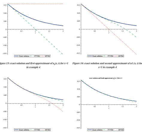
Figure 13: exact solution and first approximant of u0(x, t) for x=1 in example 4
Figure 14: exact solution and second approximant of u1 (x, t) for x=1 in example 4
Figure 15: exact solution and third approximant of u2(x, t) for
x=1 in example 4 Figure 16: exact solution and fourth approximant of u3(x, t) for x=1 in example 4
3- CONCLUSIONS
A new effective modification to the variational iteration method, the Fourier transform variational iteration method (FTVIM), is presented in this paper. The results obtained by FTVIM are compared with MVIM. The validity and effectiveness of the new method, FTVIM is shown by solving four singular differential equations with variable coefficients and the very rapid approach to the exact solutions is shown schematically. The very rapid approach towards the exact solutions of the new method, FTVIM, indicates that the amount of computational work is much less than those required for that of MVIM. Moreover, the deficiency
of the MVIM caused by unsatisfied boundary conditions is overcome by the new method, FTVIM, where, the solution is shown to be valid in the entire range of problem domain. It is concluded that the FTVIM is a powerful and efficient tool in obtaining the accurate solutions as well as other effective numerical methods.
4- REFERENCES