Volume 25 - Article 5 | Pages 173–214

(1)

Max Planck Institute for Demographic Research Konrad-Zuse Str. 1, D-18057 Rostock·GERMANY www.demographic-research.org

DEMOGRAPHIC RESEARCH

VOLUME 25, ARTICLE 5, PAGES 173-214

PUBLISHED 15 JULY 2011

http://www.demographic-research.org/Volumes/Vol25/5/ DOI: 10.4054/DemRes.2011.25.5

Research Article

Point and interval forecasts of mortality rates

and life expectancy: A comparison of

ten principal component methods

Han Lin Shang

Heather Booth

Rob J. Hyndman

c

°2011 Han Lin Shang, Heather Booth & Rob J. Hyndman.

(2)

2 Review of mortality forecasting methods 176

2.1 Lee-Carter (LC) method 176

2.2 Lee-Miller (LM) method 177

2.3 Booth-Maindonald-Smith (BMS) method 178

2.4 Hyndman-Ullah (HU) method 178

2.5 Robust Hyndman-Ullah (HUrob) method 180

2.6 Weighted Hyndman-Ullah (HUw) method 180

3 Data sets 181

4 Forecast evaluation 182

5 Comparisons of the point forecasts 182

5.1 Forecast log mortality rates 183

5.2 Forecast life expectancy 189

6 Review of interval forecast methods 194

6.1 LC methods 195

6.2 HU methods 195

6.3 Evaluating interval forecast accuracy 196

7 Comparisons of the interval forecasts 196

7.1 Forecast log mortality rates 196

7.2 Forecast life expectancy 198

8 Discussion 199

8.1 Point forecasts 199

8.2 Comparison with previous findings 203

8.3 Forecast trends in life expectancy 204

8.4 Interval forecasts 206

8.5 Effect of length of fitting period 206

8.6 Effect of robust estimation 207

8.7 Limitations 208

8.8 Implementation 209

9 Acknowledgments 209

(3)

Point and interval forecasts of mortality rates and life expectancy:

A comparison of ten principal component methods

Han Lin Shang1 Heather Booth2

Rob J. Hyndman3

Abstract

Using the age- and sex-specific data of 14 developed countries, we compare the point and interval forecast accuracy and bias of ten principal component methods for forecast-ing mortality rates and life expectancy. The ten methods are variants and extensions of the Lee-Carter method. Based on one-step forecast errors, the weighted Hyndman-Ullah method provides the most accurate point forecasts of mortality rates and the Lee-Miller method is the least biased. For the accuracy and bias of life expectancy, the weighted Hyndman-Ullah method performs the best for female mortality and the Lee-Miller method for male mortality. While all methods underestimate variability in mor-tality rates, the more complex Hyndman-Ullah methods are more accurate than the sim-pler methods. The weighted Hyndman-Ullah method provides the most accurate interval forecasts for mortality rates, while the robust Hyndman-Ullah method provides the best interval forecast accuracy for life expectancy.

1_{Department of Econometrics and Business Statistics, Monash University, Caulfield East, VIC 3145 Australia.}

E-mail: [email protected].

2_{Australian Demographic & Social Research Institute, Australian National University, ACT 0200 Australia.}

E-mail: [email protected].

(4)

1. Introduction

In recent years, the rapid ageing of the population has been a growing concern for govern-ments and societies. In many developed countries, the concerns are concentrated on the sustainability of pensions and health and aged care systems, especially given increased longevity. This has resulted in a surge of interest among government policy makers and planners in accurately modeling and forecasting age-specific mortality rates. Any im-provements in the forecast accuracy of mortality rates would be beneficial for policy decisions regarding the allocation of current and future resources. In particular, future mortality rates are of great interest to the insurance and pension industries.

Several authors have proposed new approaches for forecasting mortality rates and life expectancy using statistical modeling (see Booth 2006; Booth and Tickle 2008, for reviews). Of these, a significant milestone in demographic forecasting was the work of Lee and Carter (1992). They used a principal component method to extract a single time-varying index of the level of mortality rates, from which the forecasts are obtained using a random walk with drift. Since then, this method has been widely used for forecasting mortality rates in various countries, including Australia (Booth, Maindonald, and Smith 2002; De Jong and Tickle 2006), Austria (Carter and Prskawetz 2001), Belgium (Brouhns, Denuit, and Vermunt 2002), Canada (Lee and Nault 1993), Chile (Lee and Rofman 1994), China (Lin 1995), England & Wales (Cairns et al. 2011), Finland (Alho 1998), Japan (Wilmoth 1996), Norway (Keilman, Pham, and Hetland 2002), Spain (Felipe, Guillén, and Pérez-Marín 2002; Debón, Montes, and Sala 2006), Sweden (Lundström and Qvist 2004; Tuljapurkar 2005), the U.K. (Renshaw and Haberman 2003a), the Nordic countries (Koissi, Shapiro, and Högnäs 2006), the seven most economically developed nations (G-7) (Tuljapurkar, Li, and Boe 2000), and United State (Cairns et al. 2011).

The strengths of the Lee-Carter (LC) method are its simplicity and robustness in sit-uations where age-specific log mortality rates have linear trends (Booth et al. 2006). A weakness of the LC method is that it attempts to capture the patterns of mortality rates using only one principal component and its scores. To address this, Hyndman and Ul-lah (2007) propose a model that utilizes second and higher order principal components to capture additional dimensions of change in mortality rates. Although other methods have been developed (e.g., Renshaw and Haberman 2003a,b,c; Currie, Durban, and Eilers 2004; Bongaarts 2005; Girosi and King 2008; Renshaw and Haberman 2006; Haberman and Renshaw 2008; Ediev 2008), the LC method is often considered as the benchmark method. For example, the LC method is compared with other approaches in Cairns et al. (2011).

(5)

current forecasts (Booth, Maindonald, and Smith 2002). If a long fitting period cannot enhance forecast accuracy, the heavy data demands of the LC method can be somewhat relaxed. The question of whether or how the length of the fitting period affects point forecast accuracy was not evaluated until the works of Booth, Tickle, and Smith (2005) and Booth et al. (2006).

Several authors including Tuljapurkar, Li, and Boe (2000), Lee and Miller (2001) and Booth, Maindonald, and Smith (2002) have proposed variants of the LC method. There have also been several extensions of the LC method. Of these, the extension proposed by Hyndman and Ullah (2007) has been receiving increasing attention in the fields of de-mography and statistics. Their method combines the ideas of nonparametric smoothing, functional principal component regression and functional data analysis, in order to fore-cast mortality and fertility rates. This method has been applied by Erbas, Hyndman, and Gertig (2007) for forecasting breast cancer mortality rates in Australia. Furthermore, this method has been extended by Hyndman and Booth (2008) to improve the estimation of the variance and to include the forecasting of net migration numbers. Recently, Hyndman and Shang (2009) extended it to allow greater weight to be given to more recent data than data from the distant past.

The forecast accuracy of the LC method and its variants was first evaluated by Booth, Tickle, and Smith (2005), and further studied by Booth et al. (2006). In this article, we extend the results of Booth et al. (2006). First, we evaluate and compare the point forecast accuracy of the mortality rates and life expectancy from ten principal component methods, including methods proposed since the earlier comparison. Then, following the suggestion by Booth et al. (2006), we evaluate the forecast uncertainty of mortality rates and life ex-pectancy. Although many authors have considered the estimation of prediction intervals, particularly for medium- to long-term forecasting (e.g., Alho 1997; Tayman, Schafer, and Carter 1998; Lutz and Goldstein 2004; Alho and Spencer 2005; Brouhns, Denuit, and Van Keilegom 2005; Koissi, Shapiro, and Högnäs 2006; Haberman and Renshaw 2008; Renshaw and Haberman 2008) they do not evaluate and compare the accuracy of predic-tion intervals. To our knowledge, with the exceppredic-tion of the limited evaluapredic-tion in Booth, Tickle, and Smith (2005), an empirical comparison of the forecast uncertainty estimates has never been undertaken.

(6)

2. Review of mortality forecasting methods

In this section, we review the ten methods for forecasting mortality rates and life ex-pectancy, namely the LC method, the LC method without adjustment (LCnone), the Tuljapurkar-Li-Boe method (TLB), the Lee-Miller method (LM), the Booth-Maindonald-Smith method (BMS), the Hyndman-Ullah method (HU), the Hyndman-Ullah method using only data from 1950 onward (HU50), the robust Hyndman-Ullah method (HUrob), the robust Hyndman-Ullah method using only data from 1950 onward (HUrob50), and the weighted Hyndman-Ullah method (HUw).

We use the original notation of Lee and Carter (1992) and extend it as necessary for each method. In order to stabilize the high variance associated with high age-specific rates, it is necessary to transform the raw data by taking the natural logarithm. We denote bymx,tthe observed mortality rate at agexin yeartcalculated as the number of deaths at agexin calendar yeart, divided by the corresponding mid-year population agedx. The models and forecasts are all in log scale.

2.1 Lee-Carter (LC) method

The model structure proposed by Lee and Carter (1992) is given by

ln(mx,t) =ax+bxkt+εx,t, (1)

whereaxis the age pattern of the log mortality rates averaged across years;bxis the first principal component reflecting relative change in the log mortality rate at each age;ktis the first set of principal component scores by yeartand measures the general level of the log mortality rates; andεx,tis the residual at agexand yeart.

The LC model in (1) is over-parametrized in the sense that the model structure is invariant under the following transformations:

{ax, bx, kt} 7→ {ax, bx/c, ckt}, {ax, bx, kt} 7→ {ax−cbx, bx, kt+c}.

In order to ensure the model’s identifiability, Lee and Carter (1992) imposed two con-straints, given as:

n X

t=1

kt= 0,

xp

X

x=x1 bx= 1,

(7)

using a log transformation of the mortality rates. The adjustedkt is then extrapolated using ARIMA models. Lee and Carter (1992) used a random walk with drift model, which can be expressed as:

kt=kt−1+d+et,

wheredis known as the drift parameter and measures the average annual change in the series, andetis an uncorrelated error. It is notable that the random walk model with drift provides satisfactory results in many cases (Tuljapurkar, Li, and Boe 2000; Lee and Miller 2001; Lazar and Denuit 2009). From this forecast of the principal component scores, the forecast age-specific log mortality rates are obtained using the estimated age effectsax andbxin (1).

Two other methods are closely related to the original LC method. The first is the LC method without adjustment ofkt, labelled LCnone. The second is the TLB method, which is without adjustment and also restricts the fitting period to 1950 onward.

2.2 Lee-Miller (LM) method

The LM method is a variant of the LC method, and it differs from the LC method in three ways.

1. The fitting period begins in 1950.

2. The adjustment ofktinvolves fitting to the life expectancye(0)in yeart.

3. The jump-off rates are the actual rates in the jump-off year instead of the fitted rates.

In their evaluation of the LC method, Lee and Miller (2001) found a mismatch be-tween fitted rates for the last year of the fitting period and actual rates in that year; this jump-off error amounted to 0.6 years in life expectancy for males and females combined (Lee and Miller 2001, p.539). This jump-off error was eliminated by using actual rates in the jump-off year.

In addition, the pattern of change in mortality rates was not constant over time, which is a strong assumption of the LC method. Consequently, the adjustment of historical principal component scores resulted in a large estimation error. To overcome this, Lee and Miller (2001) adopted 1950 as the commencing year of the fitting period due to different age patterns of change for 1900-1949 and 1950-1995. This fitting period had previously been used in the TLB method.

(8)

2.3 Booth-Maindonald-Smith (BMS) method

As a variant of the LC method, the BMS method differs from the LC method in three ways.

1. The fitting period is determined on the basis of a statistical ‘goodness of fit’ crite-rion, under the assumption that the principal component scorektis linear.

2. The adjustment ofktinvolves fitting to the age distribution of deaths rather than to the total number of deaths.

3. The jump-off rates are the fitted rates under this fitting regime.

A common feature of the LC method is the linearity of the best fitting time series model of the first principal component score, but Booth, Maindonald, and Smith (2002) found the linear time series to be compromised by structural change. By first assuming the linearity of the first principal component score, the BMS method seeks to achieve the optimal ‘goodness of fit’ by selecting the optimal fitting period from all possible fitting periods ending in yearn. The optimal fitting period is determined based on the smallest ratio of the mean deviances of the fit of the underlying LC model to the overall linear fit. Instead of fitting to the total number of deaths, the BMS method fits to the age dis-tribution of deaths using the Poisson disdis-tribution to model deaths, and using deviance statistics to measure the ‘goodness of fit’ (Booth, Maindonald, and Smith 2002). The jump-off rates are taken to be the fitted rates under this adjustment.

2.4 Hyndman-Ullah (HU) method

Using the functional data analysis technique of Ramsay and Silverman (2005), Hyndman and Ullah (2007) proposed a nonparametric method for modeling and forecasting log mortality rates. It extends the LC method in three ways.

1. The log mortality rates are first smoothed using penalized regression splines with a partial monotonic constraint (see Ramsay 1988, for detail). It is assumed that there is an underlying continuous and smooth functionft(x)that is observed with error at discrete ages. To emphasize that age,x, is now considered as a continuous variable and incorporating the log transformation, we usemt(x)rather thanlnmx,t to represent the log mortality rates for agex∈[x1, xp]in yeart. Then, we can write

mt(xi) =ft(xi) +σt(xi)εt,i, i= 1, . . . , p, t= 1, . . . , n (2)

wheremt(xi)denotes the log of the observed mortality rate for age xi in yeart;

(9)

assumption of homoscedastic error in the LC model; andεt,iis an independent and identically distributed standard normal random variable.

2. More than one principal component is used. Higher order terms of the principal component decomposition improve the LC model because these additional compo-nents capture non-random patterns, which are not explained by the first principal component (Booth, Maindonald, and Smith 2002; Renshaw and Haberman 2003b; Koissi, Shapiro, and Högnäs 2006). Using functional principal component anal-ysis (FPCA), a set of curves is decomposed into orthogonal functional principal components and their uncorrelated principal component scores. That is,

ft(x) =a(x) + J X

j=1

bj(x)kt,j+et(x), (3)

wherea(x)is the mean function estimated bya(x) =ˆ 1 n

P_n

t=1ft(x);{b1(x), . . . ,

bJ(x)}is a set of the firstJfunctional principal components;{kt,1, . . . , kt,J}is a set of uncorrelated principal component scores;et(x)is the residual function with mean zero; and J < nis the number of principal components used. Following Hyndman and Booth (2008), we choseJ = 6, which should be larger than any of the components required. The conditions for the existence and uniqueness ofkt,j are discussed by Cardot, Ferraty, and Sarda (2003).

3. A wider range of univariate time series models may be used to forecast the principal component scores. By conditioning on the observed dataI={m1(x), . . . , mn(x)} and the set of functional principal componentsB = {b1(x), . . . , bJ(x)}, theh -step-ahead forecast ofmn+h(x)can be obtained by:

ˆ

mn+h|n(x) =E[mn+h(x)|I,B] = ˆa(x) + J X

j=1

bj(x)ˆkn+h|n,j,

wherekˆn+h|n,jdenotes theh-step-ahead forecast ofkn+h,jusing a univariate time series model, such as the optimal ARIMA model selected by the automatic algo-rithm of Hyndman and Khandakar (2008), or an exponential smoothing state space model (Hyndman et al. 2008). We have tried both methods, finding only a marginal difference in forecast accuracy. In this paper, we use the exponential smoothing state-space models to forecast principal component scores.

(10)

2.5 Robust Hyndman-Ullah (HUrob) method

Since the presence of outliers can seriously affect the performance of modeling and fore-casting, it is important to identify possible outliers and eliminate their effect. The robust HU method utilizes the reflection based principal component analysis (RAPCA) algo-rithm of Hubert, Rousseeuw, and Verboven (2002) to obtain projection-pursuit estimates of principal components and their associated scores. It then calculates the integrated squared error for each year, and this provides a measure of the accuracy of the princi-pal component approximation for each year (Hyndman and Ullah 2007). Outlying years would result in a larger integrated squared error than the critical value obtained by as-suming normality ofet(x)(see Hyndman and Ullah 2007, for details). By assigning zero weight to outliers, we can then apply the HU method to model and forecast mortality rates without possible influence of outliers.

The HUrob50 method is identical to the HUrob method except that the fitting period is restricted to 1950 onward.

2.6 Weighted Hyndman-Ullah (HUw) method

The HUw method adopts the same smoothing technique as the HU method, but it uses geometrically decaying weights in the estimation ofa(x)andbj(x), thus allowing these quantities to be based more on recent data than on data from the distant past.

The HUw method differs from the HU method in three ways.

1. The weighted functional meana∗_(x)_{is estimated using the weighted average}

ˆ a∗_{(x) =}

n X

t=1

wtft(x), (4)

where{wt=λ(1−λ)n−t, t= 1, . . . , n}denotes a set of weights, and0< λ <1 denotes a geometrically decaying weight parameter. Hyndman and Shang (2009) describe how to estimateλfrom data.

2. Using FPCA, a set of weighted curves{wt[ft(x)−ˆa∗(x)];t= 1, . . . , n}is decom-posed into orthogonal weighted functional principal components and their uncorre-lated principal component scores. That is,

ft(x) = ˆa∗(x) + J X

j=1

b∗j(x)kt,j+et(x), (5)

whereaˆ∗_(x)_{is the weighted functional mean, and}_{_b∗

(11)

3. By conditioning on the observed data I = {m1(x), . . . , mn(x)}and the set of weighted functional principal componentsB∗ = {b∗

1(x), . . . , b∗J(x)}, theh -step-ahead forecast ofmn+h(x)can be obtained by:

ˆ

mn+h|n(x) =E[mn+h(x)|I,B∗] = ˆa∗(x) + J X

j=1

b∗

j(x)ˆkn+h|n,j.

3. Data sets

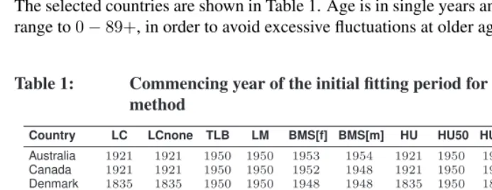
The data sets used in this study were taken from the Human Mortality Database (2009). Fourteen developed countries were selected, and thus 28 sex-specific populations were obtained for all analyses. The fourteen countries selected all have reliable data series commencing before 1950. Note that it was desirable to use only countries that have data prior to 1950, in order to maintain full and consistent comparisons of the ten methods. The selected countries are shown in Table 1. Age is in single years and we restrict the age range to0−89+, in order to avoid excessive fluctuations at older ages.

Table 1: Commencing year of the initial fitting period for each country and method

Country LC LCnone TLB LM BMS[f] BMS[m] HU HU50 HUrob HUrob50 HUw

(12)

4. Forecast evaluation

We divide each data set into a fitting period and a forecasting period. The commencing year of the fitting periods differs by method, as seen in Table 1 and also described in Section 2. We use a rolling origin as follows: The forecasting period is initially set to be the last 30 years, ending in 2004. Using the data in the fitting period, we compute one-step-ahead and ten-step-ahead point forecasts, and determine the forecast errors by comparing the forecasts with the actual out-of-sample data. Then, we increase the fit-ting period by one year, and compute one-step-ahead and ten-step-ahead forecasts, and calculate the forecast errors. This process is repeated until the fitting period extends to 2003.

For the BMS method, the initial optimal fitting period is based on the goodness of fit criterion using data up to 1974; Table 1 shows the resulting commencing years. Com-mencing years differ between the sexes as a result of independently selecting the optimal fitting period. As the fitting period is increased by one year, the optimal fitting period is re-estimated for each increment (commencing years not shown). This may result in substantial changes in the commencing year, which may increase or decrease the length of the fitting period.

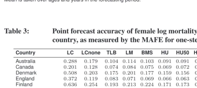
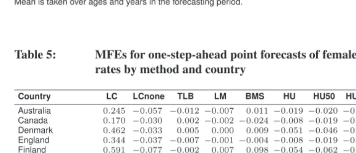
Using thedemographypackage for R (Hyndman 2011), we calculate the point and interval forecasts of each method, and evaluate and compare their forecast accuracy. To measure point forecast accuracy, we utilize the mean absolute forecast error (MAFE) and the mean forecast error (MFE). The MAFE is the average of absolute errors,|actual− forecast|, and measures forecast precision, regardless of sign. The MFE is the average of errors,(actual−forecast), and is a measure of bias. These measures are used to evaluate forecasts of log mortality rates and life expectancy.

5. Comparisons of the point forecasts

(13)

5.1 Forecast log mortality rates

Tables 2 and 3 provide summaries of the point forecast accuracy based on the MAFEs for one-step-ahead forecasts of mortality rates averaged over different ages and years in the forecasting period for males and females respectively. As measured by the simple and weighted averages of MAFE over countries, the HU methods tend to perform better than the LC methods, and the HUw method performs the best in the male and female data. The HUw method also performs at least as well as any other method in 26 of the 28 populations.

Tables 4 and 5 show the corresponding MFEs for one-step-ahead forecasts. For both male and female rates, all HU methods overestimate mortality consistently for all coun-tries. Among these methods, the HU50 method performs best for male rates, according to both the simple and weighted averages, while the HUw method performs best for female rates. Among the LC methods, there is less consistency. The LM method performs best overall, though the BMS method has the lowest simple average for male rates. The LC method underestimates female rates for all 14 countries and male rates for 11 of the 14 countries.

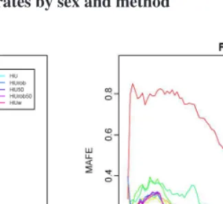
Figures 1a and 1b show the MAFEs for one-step-ahead forecasts for different meth-ods averaged over unweighted countries and years in the forecasting period for male and female mortality rates respectively. Larger errors occur at younger ages (less than 40 at least) for all methods, reflecting the difficulty in capturing both the nadir of the mortality schedule and the accident hump; errors from the LC method are particularly large at these ages. At older ages, errors from the LCnone method are large relative to all other meth-ods. Contributing to their lower average MAFEs in Tables 2 and 3, the HU methods tend to be more accurate than most LC methods at most ages.

(14)

Table 2: Point forecast accuracy of male log mortality rates by method and country, as measured by the MAFE for one-step-ahead forecasts

Country LC LCnone TLB LM BMS HU HU50 HUrob HUrob50 HUw

Australia 0.388 0.183 0.110 0.092 0.093 0.079 0.079 0.105 0.092 0.076 Canada 0.246 0.133 0.088 0.069 0.079 0.060 0.061 0.090 0.077 0.057 Denmark 0.185 0.180 0.152 0.157 0.145 0.127 0.127 0.143 0.136 0.123 England 0.545 0.175 0.085 0.058 0.088 0.062 0.054 0.083 0.063 0.052 Finland 0.445 0.211 0.150 0.156 0.140 0.141 0.133 0.147 0.137 0.131 France 0.450 0.180 0.083 0.054 0.102 0.064 0.050 0.115 0.061 0.050 Iceland 0.328 0.326 0.328 0.407 0.327 0.332 0.350 0.337 0.344 0.335 Italy 0.283 0.168 0.111 0.065 0.111 0.075 0.062 0.113 0.083 0.061 Netherlands 0.148 0.133 0.110 0.093 0.111 0.081 0.078 0.095 0.084 0.078 Norway 0.235 0.171 0.151 0.150 0.140 0.118 0.120 0.133 0.127 0.120 Scotland 0.649 0.215 0.141 0.152 0.131 0.124 0.121 0.130 0.121 0.118 Spain 0.243 0.158 0.112 0.067 0.113 0.065 0.064 0.072 0.075 0.058 Sweden 0.191 0.171 0.142 0.140 0.137 0.118 0.115 0.146 0.123 0.114 Switzerland 0.225 0.183 0.131 0.136 0.131 0.116 0.113 0.132 0.122 0.112

Average 0.326 0.185 0.135 0.128 0.132 0.112 0.109 0.131 0.118 0.106

Weighted average 0.351 0.168 0.103 0.075 0.105 0.074 0.067 0.102 0.080 0.065

Mean is taken over ages and years in the forecasting period.

Table 3: Point forecast accuracy of female log mortality rates by method and country, as measured by the MAFE for one-step-ahead forecasts

Average 0.426 0.192 0.148 0.156 0.170 0.129 0.128 0.151 0.131 0.124

(15)

Table 4: MFEs for one-step-ahead point forecasts of male log mortality rates by method and country

Country LC LCnone TLB LM BMS HU HU50 HUrob HUrob50 HUw

Australia 0.311 −0.076 −0.030 −0.013 −0.008−0.025 −0.016 −0.034 −0.020 −0.024 Canada 0.171 −0.058 −0.035 −0.011 −0.020−0.017 −0.017 −0.026 −0.023 −0.015 Denmark 0.018 0.030 −0.046 −0.008 −0.024−0.034 −0.046 −0.037 −0.060 −0.036 England 0.495 −0.065 −0.011 −0.006 0.028−0.031 −0.014 −0.033 −0.018 −0.021 Finland 0.365 −0.076 −0.024 −0.004 −0.003−0.064 −0.044 −0.058 −0.048 −0.058 France 0.389 −0.082 −0.028 −0.010 0.020−0.036 −0.013 −0.041 −0.017 −0.030 Iceland −0.059 −0.059 −0.061 −0.011 −0.044−0.153 −0.210 −0.164 −0.196 −0.171 Italy 0.210 −0.033 −0.039 −0.007 0.042−0.035 −0.015 −0.037 −0.018 −0.027 Netherlands −0.039 0.018 −0.053 −0.008 −0.028−0.035 −0.019 −0.033 −0.024 −0.031 Norway 0.011 0.004 −0.053 −0.009 −0.035−0.041 −0.036 −0.044 −0.047 −0.039 Scotland 0.584 −0.051 −0.000 −0.004 0.010−0.037 −0.042 −0.039 −0.040 −0.038 Spain 0.192 −0.015 0.003 0.004 0.055−0.007 −0.027 −0.009 −0.025 −0.009 Sweden −0.039 0.015 −0.045 −0.010 0.005−0.055 −0.044 −0.058 −0.050 −0.055 Switzerland 0.151 −0.027 −0.014 −0.009 −0.001−0.041 −0.043 −0.047 −0.049 −0.041

Average 0.197 −0.034 −0.031 −0.007 0.000−0.044 −0.042 −0.047 −0.045 −0.043

Weighted average 0.272 −0.045 −0.025 −0.007 0.019−0.030 −0.020 −0.033 −0.023 −0.025

Table 5: MFEs for one-step-ahead point forecasts of female log mortality rates by method and country

Australia 0.245 −0.057 −0.012 −0.007 0.011−0.019 −0.020 −0.026 −0.023 −0.022 Canada 0.170 −0.030 0.002 −0.002 −0.024−0.008 −0.019 −0.009 −0.018 −0.009 Denmark 0.462 −0.033 0.005 0.000 0.009−0.051 −0.046 −0.055 −0.057 −0.047 England 0.344 −0.037 −0.007 −0.001 −0.004−0.008 −0.019 −0.013 −0.021 −0.007 Finland 0.591 −0.077 −0.002 0.007 0.098−0.054 −0.062 −0.058 −0.059 −0.052 France 0.488 −0.077 −0.006 −0.002 0.085−0.022 −0.013 −0.031 −0.013 −0.016 Iceland 0.100 −0.100 −0.158 0.007 0.082−0.133 −0.161 −0.131 −0.138 −0.123 Italy 0.332 −0.043 −0.015 0.001 0.046−0.017 −0.019 −0.019 −0.020 −0.016 Netherlands 0.339 −0.032 0.012 0.001 0.028−0.019 −0.013 −0.019 −0.016 −0.017 Norway 0.528 −0.037 0.005 0.004 0.103−0.038 −0.053 −0.050 −0.046 −0.038 Scotland 0.485 −0.045 −0.009 0.006 0.015−0.050 −0.067 −0.056 −0.063 −0.046 Spain 0.398 −0.051 −0.019 0.010 0.081−0.004 −0.030 −0.005 −0.032 −0.004 Sweden 0.349 −0.034 0.005 0.001 0.216−0.063 −0.042 −0.087 −0.041 −0.060 Switzerland 0.350 −0.045 0.006 0.002 0.029−0.044 −0.050 −0.048 −0.050 −0.041

Average 0.370 −0.050 −0.014 0.002 0.055−0.038 −0.044 −0.043 −0.043 −0.035

Weighted average 0.364 −0.049 −0.007 0.001 0.045−0.018 −0.023 −0.023 −0.024 −0.016

(16)

Figure 1: MAFEs and MFEs for one-step-ahead point forecasts of log mortality rates by sex and method

(a) MAFEs averaged over years in the forecasting period, and countries

(b) MAFEs averaged over years in the forecasting period, and countries

(c) MFEs averaged over years in the forecasting period, and countries

(17)

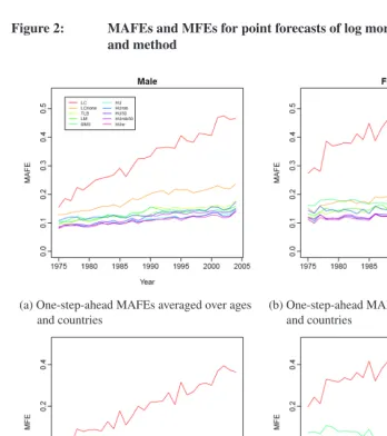
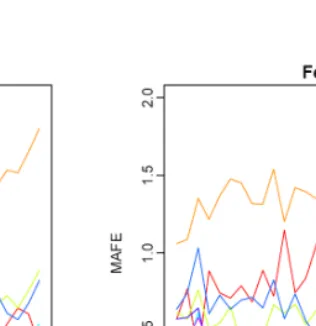
Figures 2a and 2b show the MAFEs for one-step-ahead point forecasts from different methods averaged over countries and ages for male and female mortality respectively. The trend in these measures indicates that it is marginally increasingly difficult to forecast the mortality for later years. Further, differences in the patterns of fluctuation by method in-dicate that the degree of difficulty is not only dependent on the particular annual mortality experience.

Figures 2c and 2d similarly show the MFEs for one-step-ahead forecasts. For most methods, bias is very small though a slight trend towards overestimation in later years occurs for the HU methods and some LC methods. In contrast, the LC method tends strongly towards underestimation in later years. The LM method displays no trend for either sex. In interpreting these one-step-ahead values, it should be borne in mind that they are significantly influenced by jump-off error and by random error in the particular year (seen in the common pattern of fluctuation). The absence of jump-off error in the LM method helps to explain the relative accuracy of this method (see also Section 8.1).

(18)

Figure 2: MAFEs and MFEs for point forecasts of log mortality rates by sex and method

(a) One-step-ahead MAFEs averaged over ages and countries

(b) One-step-ahead MAFEs averaged over ages and countries

(c) One-step-ahead MFEs averaged over ages and countries

(19)

Figure 2: (Continued)

(e) Ten-step-ahead MFEs averaged over ages and countries

(f) Ten-step-ahead MFEs averaged over ages and countries

5.2 Forecast life expectancy

(20)

Table 6: Point forecast accuracy of male life expectancy by method and country, as measured by the MAFE for one-step-ahead forecasts

Average 0.632 1.259 0.625 0.237 0.359 0.474 0.417 0.637 0.468 0.354

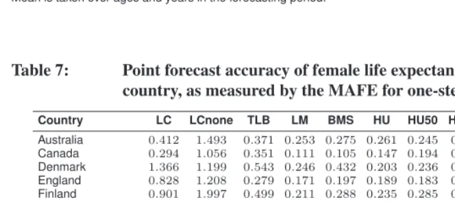
Table 7: Point forecast accuracy of female life expectancy by method and country, as measured by the MAFE for one-step-ahead forecasts

Average 0.818 1.483 0.608 0.242 0.316 0.347 0.379 0.582 0.360 0.272

(21)

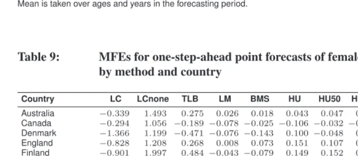
Corresponding MFEs for one-step-ahead point forecasts of life expectancy are shown in Tables 8 and 9. In general, average underestimation in mortality rates does not nec-essarily translate into overestimation in life expectancy and vice versa, because of the implicit weights applied to errors by age. However, there is a clear association between differences in the age patterns in forecast errors and differences in the size and sign of forecast errors in life expectancy. For both sexes, all HU methods and the LCnone (in particular) and TLB methods tend to underestimate life expectancy, both on average and almost consistently across countries, while the LC method overestimates life expectancy on average and for most countries. Based on the simple and weighted averages, the LM method is superior for male life expectancy, while for female life expectancy the HUw method is superior according to the weighted average and the BMS method is superior according to the simple average.

Figures 3a and 3b display the MAFEs for one-step-ahead point forecasts of life ex-pectancy by years in the forecasting period for males and females respectively. For both sexes, all methods except LCnone are roughly equally accurate over years in the forecast-ing period, and LM is the most accurate in most years. For life expectancy, the outlier is LCnone rather than LC. This arises from the relatively large errors at older ages which have a greater effect on life expectancy (at low levels of mortality), whereas the LC ad-justment produces relatively large errors at young ages.

(22)

Table 8: MFEs for one-step-ahead point forecasts of male life expectancy by method and country

Australia −0.570 1.836 0.687 0.171 0.235 0.256 0.124 0.493 0.228 0.210 Canada −0.179 1.326 0.484 0.120 0.251 0.161 0.187 0.394 0.265 0.124 Denmark 0.216 0.036 0.527 0.092 0.360 0.253 0.276 0.518 0.497 0.110 England −0.914 1.837 0.486 0.113 0.151 0.491 0.136 0.633 0.244 0.225 Finland −0.571 1.861 0.569 0.077 0.166 0.540 0.248 0.471 0.361 0.367 France −0.921 2.298 0.282 0.079 0.109 0.522 0.137 1.032 0.145 0.291 Iceland 0.447 0.377 0.918 0.589 0.835 1.494 2.081 1.630 1.921 1.468 Italy −0.047 1.405 0.913 0.123 0.167 0.606 0.177 0.916 0.283 0.257 Netherlands 0.310 −0.213 0.769 0.121 0.555 0.314 0.188 0.212 0.259 0.219 Norway 0.364 0.094 0.895 0.141 0.527 0.309 0.223 0.382 0.361 0.190 Scotland −1.257 1.728 0.429 0.096 0.068 0.412 0.323 0.456 0.288 0.223 Spain −0.381 1.264 0.661−0.008−0.064 0.247 0.349 0.381 0.374 0.062 Sweden 0.291 −0.311 0.573 0.108 0.197 0.409 0.292 0.626 0.385 0.315 Switzerland −0.468 0.921 0.187 0.078 0.058 0.291 0.253 0.433 0.368 0.210

Average −0.263 1.033 0.598 0.136 0.258 0.450 0.357 0.613 0.427 0.305

Weighted average −0.445 1.472 0.578 0.095 0.161 0.414 0.196 0.655 0.269 0.213

Table 9: MFEs for one-step-ahead point forecasts of female life expectancy by method and country

Australia −0.339 1.493 0.275 0.026 0.018 0.043 0.047 0.131 0.081 0.054 Canada −0.294 1.056 −0.189−0.078−0.025 −0.106−0.032−0.145 −0.060 −0.073 Denmark −1.366 1.199 −0.471−0.076−0.143 0.100−0.048 0.436 0.059 0.012 England −0.828 1.208 0.268 0.008 0.073 0.151 0.107 0.464 0.148 0.026 Finland −0.901 1.997 0.484−0.043−0.079 0.149 0.152 0.266 0.124 0.078 France −0.983 2.212 0.177−0.046−0.206 0.181 0.031 0.905 0.040 0.031 Iceland 0.142 1.663 2.289 0.728 0.978 1.724 2.074 1.562 1.732 1.374 Italy −0.419 1.655 0.622−0.008−0.075 0.238 0.110 0.479 0.154 0.094 Netherlands −0.811 1.216 −0.252−0.079−0.167 −0.027−0.071−0.031 −0.123 −0.016 Norway −1.065 1.254 0.314−0.029−0.176 0.236 0.282 0.586 0.204 0.060 Scotland −1.158 1.442 0.517−0.003 0.110 0.331 0.368 0.749 0.314 0.108 Spain −0.587 1.720 1.031−0.051−0.028 0.135 0.168 0.248 0.272 −0.036 Sweden −0.942 0.958 −0.226−0.066−0.248 0.280 0.027 0.948 −0.059 0.176 Switzerland −0.793 1.575 0.040−0.067−0.164 0.091 0.086 0.268 0.012 −0.032

Average −0.739 1.475 0.349 0.015−0.009 0.252 0.236 0.490 0.207 0.133

Weighted average −0.688 1.572 0.324−0.031−0.069 0.136 0.078 0.429 0.100 0.027

(23)

Figure 3: MFEs and MAFEs for point forecasts of life expectancy by sex and method

(a) One-step-ahead MAFEs averaged over countries

(b) One-step-ahead MAFEs averaged over countries

(c) One-step-ahead MFEs averaged over countries

(24)

Figure 3: (Continued)

(e) Ten-step-ahead MFEs averaged over countries

(f) Ten-step-ahead MFEs averaged over countries

6. Review of interval forecast methods

Prediction intervals are a valuable tool for assessing the probabilistic uncertainty associ-ated with point forecasts. As was emphasized by Chatfield (1993, 2000), it is important to provide interval forecasts as well as point forecasts, so as to

1. assess future uncertainty levels;

2. enable different strategies to be planned for the range of possible outcomes indi-cated by the interval forecasts;

3. compare forecasts from different methods more thoroughly; and 4. explore different scenarios based on different assumptions.

(25)

6.1 LC methods

In Lee and Carter (1992), the LC method considers only the uncertainty in the innovations. Although Lee and Carter (1992, p.665) acknowledged that the inclusion of uncertainty in the drift would increase the standard error of their forecasts by 25% after 50 years (based on the period from 1900 to 1989), they did not include it. Booth, Maindonald, and Smith (2002) included the uncertainty in the drift, and compared the variances for the LC, LM and BMS methods with and without this additional uncertainty.

We consider two sources of uncertainty: errors in the parameter estimation of the LC models and forecast errors in the projected time series coefficients. Because of the orthogonality between the first principal component and the error term in (1), the overall forecast variance can be approximated by the sum of the two variances. Conditioning on the observed dataIand the first principal componentbx, we obtained the overall forecast variance oflnmx,t,

Var[lnmx,t]≈b2xun+h|n+vx, whereb2

xis the variance of the first principal component;un+h|n =Var(kn+h|k1, . . . , kn) can be obtained from the time series model; and the model residual variancevxis esti-mated by averaging the residual squares{ε2

x,1, . . . , ε2x,n}for eachxin (1).

6.2 HU methods

The forecast variance follows from (2) and (3). Due to the orthogonality between the prin-cipal components and the error term, the overall forecast variance can be approximated by the sum of four variances. Conditioning on the observed dataI and the set of fixed principal componentsB={b1(x), . . . , bJ(x)}, we obtained the overall forecast variance ofmn+h(x),

Var[mn+h(x)|I,B]≈ˆσa2(x) + J X

j=1

b2j(x)un+h|n,j+v(x) +σn2+h(x),

whereσˆ2

a(x)(the variance of the smooth estimatea(x)ˆ ) can be obtained from the smooth-ing method used in (2);b2

j(x)is the variance of thejthprincipal component;un+h|n,j = Var(kn+h,j|k1,j, . . . , kn,j)can be obtained from the time series model; the model residual variancev(x)is estimated by averaging{e2

1(x), . . . , e2n(x)}for eachx; and the observa-tional error varianceσ2

n+h(x)is estimated by averaging{σˆ12(x), . . . ,σˆ2n(x)}for eachx (Hyndman and Ullah 2007).

(26)

con-6.3 Evaluating interval forecast accuracy

The method of evaluation of interval forecast accuracy for mortality rates is as follows: Variances for the LC methods were calculated as described in Section 6.1, and variances for all HU methods were calculated as described in Section 6.2. For each year in the forecasting period, one-step-ahead prediction intervals were calculated at the 0.8 nominal coverage probability, and were then tested against the actual proportion of out-of-sample data that fell within the calculated prediction intervals (Swanson and Beck 1994; Tayman, Smith, and Lin 2007). The empirical coverage probability is defined as the proportion of observations that fall into the calculated 80% prediction intervals, where the denominator is the total number of observations in the forecasting period (for example, 90 ages×30 years = 2700 observations). We calculated the coverage probability deviance, which is the absolute difference between the nominal coverage probability and the empirical coverage probability, and use this measure to evaluate the interval forecast accuracy of each method. With a nominal coverage probability of 0.8, the maximum coverage probability deviance is 0.8 (i.e., when the empirical coverage probability is 0), while the minimum coverage probability deviance is 0 (i.e., when the empirical coverage probability is 0.8). Results are presented in terms of the coverage probability deviance.

To obtain prediction intervals for future life expectancies, we simulated the forecast log mortality rates as described in Hyndman and Booth (2008). In short, the simulated forecasts of log mortality rates were obtained by adding disturbances to the forecast time series coefficients which were then multiplied by the fixed principal components. Life expectancy was then calculated for each set of simulated log mortality rates. Prediction intervals were constructed from the 80% percentiles of the simulated life expectancies. In this case, the empirical probability coverage and the coverage probability deviance were based on 30 observations (one for each year in the forecasting period).

7. Comparisons of the interval forecasts

7.1 Forecast log mortality rates

(27)

Of the HU methods, the HU50 and HUrob50 methods perform least well. Their com-parison with the HU and HUrob methods indicates that restricting the fitting period to 1950 onward does not provide a more accurate estimate of forecast uncertainty.

Table 10: Coverage probability deviances of forecasted male log mortality rates by method and country

Country LC LCnone TLB LM BMS

Australia 0.710(−) 0.710(−) 0.720(−) 0.509(−) 0.605(−) Canada 0.739(−) 0.667(−) 0.690(−) 0.642(−) 0.710(−) Denmark 0.577(−) 0.594(−) 0.747(−) 0.735(−) 0.756(−) England 0.640(−) 0.467(−) 0.663(−) 0.463(−) 0.597(−) Finland 0.650(−) 0.538(−) 0.602(−) 0.423(−) 0.668(−) France 0.684(−) 0.409(−) 0.673(−) 0.562(−) 0.640(−) Iceland 0.421(−) 0.490(−) 0.590(−) 0.710(−) 0.497(−) Italy 0.465(−) 0.425(−) 0.638(−) 0.427(−) 0.633(−) Netherlands 0.208(−) 0.274(−) 0.625(−) 0.562(−) 0.535(−) Norway 0.584(−) 0.580(−) 0.710(−) 0.706(−) 0.746(−) Scotland 0.642(−) 0.649(−) 0.688(−) 0.642(−) 0.542(−) Spain 0.567(−) 0.441(−) 0.602(−) 0.404(−) 0.629(−) Sweden 0.390(−) 0.364(−) 0.668(−) 0.657(−) 0.706(−) Switzerland 0.591(−) 0.580(−) 0.650(−) 0.678(−) 0.679(−)

Average 0.562(−) 0.514(−) 0.662(−) 0.580(−) 0.639(−)

Weighted average 0.589(−) 0.478(−) 0.658(−) 0.514(−) 0.635(−)

Country HU HU50 HUrob HUrob50 HUw

Australia 0.226(−) 0.306(−) 0.259(−) 0.324(−) 0.134(−) Canada 0.389(−) 0.454(−) 0.445(−) 0.464(−) 0.205(−) Denmark 0.219(−) 0.470(−) 0.236(−) 0.471(−) 0.163(−) England 0.066(−) 0.358(−) 0.013(−) 0.397(−) 0.144(+) Finland 0.226(−) 0.510(−) 0.179(−) 0.512(−) 0.164(−) France 0.116(−) 0.419(−) 0.154(−) 0.381(−) 0.130(+) Iceland 0.287(−) 0.479(−) 0.294(−) 0.470(−) 0.270(−) Italy 0.060(−) 0.328(−) 0.037(−) 0.379(−) 0.165(+) Netherlands 0.167(−) 0.536(−) 0.184(−) 0.516(−) 0.120(−) Norway 0.222(−) 0.405(−) 0.233(−) 0.442(−) 0.205(−) Scotland 0.451(−) 0.590(−) 0.433(−) 0.582(−) 0.352(−) Spain 0.178(−) 0.451(−) 0.133(−) 0.443(−) 0.133(−) Sweden 0.310(−) 0.626(−) 0.402(−) 0.657(−) 0.032(+) Switzerland 0.437(−) 0.554(−) 0.440(−) 0.531(−) 0.283(−)

Average 0.239(−) 0.463(−) 0.246(−) 0.469(−) 0.179(−)

(28)

Table 11: Coverage probability deviances of forecasted female log mortality rates by method and country

Australia 0.572(−) 0.680(−) 0.633(−) 0.448(−) 0.541(−) Canada 0.624(−) 0.669(−) 0.544(−) 0.601(−) 0.628(−) Denmark 0.720(−) 0.572(−) 0.592(−) 0.644(−) 0.668(−) England 0.704(−) 0.404(−) 0.573(−) 0.338(−) 0.452(−) Finland 0.731(−) 0.625(−) 0.656(−) 0.622(−) 0.667(−) France 0.701(−) 0.387(−) 0.583(−) 0.426(−) 0.499(−) Iceland 0.396(−) 0.540(−) 0.558(−) 0.673(−) 0.476(−) Italy 0.574(−) 0.269(−) 0.565(−) 0.403(−) 0.473(−) Netherlands 0.601(−) 0.394(−) 0.439(−) 0.499(−) 0.517(−) Norway 0.739(−) 0.572(−) 0.625(−) 0.639(−) 0.653(−) Scotland 0.722(−) 0.617(−) 0.656(−) 0.589(−) 0.547(−) Spain 0.622(−) 0.437(−) 0.616(−) 0.453(−) 0.639(−) Sweden 0.641(−) 0.349(−) 0.566(−) 0.546(−) 0.644(−) Switzerland 0.670(−) 0.592(−) 0.587(−) 0.651(−) 0.664(−)

Average 0.644(−) 0.508(−) 0.585(−) 0.538(−) 0.576(−)

Australia 0.262(−) 0.307(−) 0.298(−) 0.302(−) 0.046(−) Canada 0.278(−) 0.388(−) 0.246(−) 0.403(−) 0.079(−) Denmark 0.326(−) 0.471(−) 0.359(−) 0.486(−) 0.197(−) England 0.051(−) 0.349(−) 0.120(−) 0.360(−) 0.097(+) Finland 0.445(−) 0.534(−) 0.423(−) 0.503(−) 0.316(−) France 0.080(−) 0.434(−) 0.169(−) 0.416(−) 0.137(+) Iceland 0.307(−) 0.474(−) 0.301(−) 0.460(−) 0.300(−) Italy 0.003(+) 0.376(−) 0.070(−) 0.383(−) 0.144(+) Netherlands 0.194(−) 0.430(−) 0.216(−) 0.388(−) 0.161(−) Norway 0.317(−) 0.429(−) 0.392(−) 0.382(−) 0.129(−) Scotland 0.373(−) 0.452(−) 0.399(−) 0.482(−) 0.310(−) Spain 0.139(−) 0.462(−) 0.122(−) 0.484(−) 0.089(−) Sweden 0.277(−) 0.561(−) 0.283(−) 0.491(−) 0.054(−) Switzerland 0.395(−) 0.518(−) 0.418(−) 0.507(−) 0.379(−)

Average 0.246(−) 0.442(−) 0.272(−) 0.432(−) 0.174(−)

Mean is taken over different ages and years in the forecasting period. Minus sign indicates that the empirical co-verage probability is less than the nominal coco-verage probability. Plus sign indicates that the empirical coco-verage probability is greater than the nominal coverage probability.

7.2 Forecast life expectancy

(29)

relative to the HU methods. The superior performance of the HU methods can be at-tributed to the consideration of four sources of uncertainty. Most HU methods also have negative average coverage probability deviances, but positive country-specific values are much more frequent. The HUw method is unique in producing prediction intervals that are consistently too wide across all populations. It is noted that restriction of the fitting period to 1950 onwards results in a loss of accuracy for male life expectancy (as might be expected from the similar result for log mortality rates) but not for female life expectancy.

8. Discussion

The above comparative analysis of mortality forecasting methods is the most comprehen-sive to date. It constitutes an evaluation of point and interval forecasts for log mortality rates and life expectancy based on ten principal component methods and 28 populations. The methods include the LC method and four LC variants, and the HU method, itself an extension of LC method, and four HU variants. The evaluation of point forecasts is an expansion of Booth et al. (2006). The evaluation of interval forecast accuracy is novel in demographic forecasting, though we acknowledge the early contribution of Booth, Main-donald, and Smith (2002); Booth, Tickle, and Smith (2005) in relation to the LC, LM and BMS methods.

8.1 Point forecasts

Our overall findings regarding point forecasts of mortality rates are that the HUw method is more accurate than any other method for one-step-ahead forecasts (Tables 2 and 3), and that the LM method is the least biased (Tables 4 and 5). The success of the HUw method suggests that attributing greater weight to the recent past leads to generally smaller age-specific errors, given that such errors are cumulated in MAFE.

(30)

Table 12: Coverage probability deviances of forecasted male life expectancy by method and country

Australia 0.400(−) 0.800(−) 0.800(−) 0.067(−) 0.267(−) Canada 0.133(−) 0.800(−) 0.800(−) 0.700(−) 0.700(−) Denmark 0.400(−) 0.167(−) 0.733(−) 0.633(−) 0.733(−) England 0.400(−) 0.700(−) 0.800(−) 0.333(−) 0.400(−) Finland 0.033(−) 0.800(−) 0.800(−) 0.367(−) 0.600(−) France 0.067(+) 0.800(−) 0.800(−) 0.667(−) 0.733(−) Iceland 0.167(−) 0.100(−) 0.433(−) 0.533(−) 0.167(−) Italy 0.067(−) 0.567(−) 0.800(−) 0.167(+) 0.167(+) Netherlands 0.067(−) 0.033(+) 0.800(−) 0.700(−) 0.700(−) Norway 0.433(−) 0.400(−) 0.700(−) 0.667(−) 0.800(−) Scotland 0.700(−) 0.800(−) 0.800(−) 0.600(−) 0.267(−) Spain 0.367(−) 0.800(−) 0.800(−) 0.267(−) 0.600(−) Sweden 0.300(−) 0.067(−) 0.733(−) 0.700(−) 0.733(−) Switzerland 0.033(−) 0.700(−) 0.700(−) 0.667(−) 0.667(−)

Average 0.255(−) 0.538(−) 0.750(−) 0.505(−) 0.538(−)

Australia 0.067(+) 0.067(+) 0.167(+) 0.100(+) 0.200(+) Canada 0.033(−) 0.200(−) 0.333(−) 0.233(−) 0.167(+) Denmark 0.100(−) 0.300(−) 0.067(−) 0.333(−) 0.200(+) England 0.200(+) 0.100(−) 0.100(+) 0.233(−) 0.200(+) Finland 0.067(−) 0.567(−) 0.067(+) 0.567(−) 0.100(+) France 0.200(+) 0.267(−) 0.067(−) 0.067(−) 0.200(+) Iceland 0.200(+) 0.400(−) 0.200(+) 0.400(−) 0.200(+) Italy 0.173(+) 0.167(+) 0.171(+) 0.167(+) 0.200(+) Netherlands 0.067(+) 0.633(−) 0.000(+) 0.600(−) 0.200(+) Norway 0.067(−) 0.233(−) 0.033(+) 0.367(−) 0.200(+) Scotland 0.700(−) 0.800(−) 0.600(−) 0.767(−) 0.200(+) Spain 0.067(−) 0.333(−) 0.000(+) 0.233(−) 0.200(+) Sweden 0.200(+) 0.700(−) 0.000(+) 0.633(−) 0.200(+) Switzerland 0.400(−) 0.533(−) 0.400(−) 0.500(−) 0.200(+)

Average 0.181(−) 0.379(−) 0.157(−) 0.371(−) 0.190(+)

Weighted average 0.152(−) 0.261(−) 0.126(−) 0.236(−) 0.195(+)

(31)

Table 13: Coverage probability deviances of forecasted female life expectancy by method and country

Australia 0.167(−) 0.800(−) 0.667(−) 0.000 0.200(−) Canada 0.067(+) 0.800(−) 0.267(−) 0.133(−) 0.333(−) Denmark 0.600(−) 0.800(−) 0.000 0.267(−) 0.433(−) England 0.467(−) 0.767(−) 0.800(−) 0.000 0.067(−) Finland 0.300(−) 0.800(−) 0.800(−) 0.533(−) 0.433(−) France 0.267(−) 0.800(−) 0.700(−) 0.200(−) 0.133(−) Iceland 0.067(−) 0.200(−) 0.233(−) 0.333(−) 0.133(−) Italy 0.067(−) 0.767(−) 0.800(−) 0.100(−) 0.133(−) Netherlands 0.400(−) 0.800(−) 0.100(−) 0.100(−) 0.200(−) Norway 0.567(−) 0.800(−) 0.767(−) 0.433(−) 0.533(−) Scotland 0.800(−) 0.800(−) 0.800(−) 0.333(−) 0.367(−) Spain 0.500(−) 0.800(−) 0.800(−) 0.400(−) 0.400(−) Sweden 0.133(−) 0.767(−) 0.567(−) 0.367(−) 0.333(−) Switzerland 0.033(−) 0.800(−) 0.500(−) 0.533(−) 0.467(−)

Average 0.317(−) 0.750(−) 0.557(−) 0.267(−) 0.298(−)

Australia 0.033(−) 0.167(−) 0.133(+) 0.033(+) 0.200(+) Canada 0.200(−) 0.400(−) 0.300(−) 0.333(−) 0.133(+) Denmark 0.200(+) 0.100(+) 0.200(+) 0.067(+) 0.200(+) England 0.200(+) 0.200(+) 0.200(+) 0.200(+) 0.200(+) Finland 0.033(+) 0.300(−) 0.033(+) 0.167(−) 0.100(+) France 0.200(+) 0.033(+) 0.133(+) 0.033(+) 0.200(+) Iceland 0.200(+) 0.033(−) 0.200(+) 0.033(−) 0.200(+) Italy 0.200(+) 0.067(+) 0.033(+) 0.133(+) 0.200(+) Netherlands 0.167(+) 0.067(+) 0.167(+) 0.067(+) 0.167(+) Norway 0.200(+) 0.033(−) 0.100(+) 0.133(+) 0.200(+) Scotland 0.033(+) 0.300(−) 0.067(−) 0.333(−) 0.133(+) Spain 0.100(+) 0.000 0.033(+) 0.100(+) 0.200(+) Sweden 0.200(+) 0.233(−) 0.167(+) 0.133(−) 0.200(+) Switzerland 0.133(+) 0.133(+) 0.067(+) 0.133(+) 0.167(+)

Average 0.150(+) 0.148(−) 0.131(+) 0.136(+) 0.179(+)

Weighted average 0.167(+) 0.127(−) 0.127(+) 0.129(+) 0.188(+)

(32)

The success, in terms of bias, of the LM method stems from the cancellation in MFE of errors across age, years in the forecasting period, and country (if applicable). Can-cellation across age (and country) is seen to be advantageous (Figures 2c and 2d), while cancellation across years in the forecasting period (and country) is seen to be even more advantageous (Figures 1c and 1d). However, the cancellation of one-step-ahead errors over years in the forecasting period occurs to a greater degree in the LM method than in any other method because of the simple linear time series model and the absence of jump-off error. Thus the superior performance of the LM method with respect to bias is mainly an artefact of averaging over one-step-ahead errors based on a rolling origin, and may not be true in other circumstances (e.g., longer forecast horizons). Among the nine remaining methods, the BMS method performs best for male mortality and the TLB method for female mortality.

For life expectancy, the cancellation of errors across age occurs in its calculation, thus affecting MAFE as well as MFE, prior to averaging over years in the forecasting period and country. Further, for the LM method, averaging over years in the forecasting period is less directly instrumental in reducing bias (than in the case of rates). On balance, the LM method is ranked first on both MAFE and MFE for male life expectancy, while the HUw method is ranked first on both MAFE and MFE for female life expectancy based on weighted averages.

Regarding the direction of bias, all HU methods show a tendency towards one-step-ahead overestimation of mortality rates (Tables 4 and 5), and a related tendency towards underestimation of life expectancy, particularly for male mortality (Tables 8 and 9). Sim-ilar findings occur for the LCnone and TLB methods. In contrast, the LC method exhibits a strong tendency towards one-step-ahead underestimation of mortality rates, usually pro-ducing the overestimation of life expectancy, especially for female mortality. The small LM biases tend towards overestimation in male mortality and underestimation in female mortality. For ten-step-ahead forecasts of mortality rates, there is a tendency towards greater overestimation in all HU methods, and for male mortality in all LC methods.

These biases are better understood in terms of age patterns of errors (Figures 1c and 1d). For all methods, one-step-ahead errors are smaller at older than younger ages, and overestimation occurs at older ages. No method captures the rapidity of mortality decline at older ages, contributing to the tendency to underestimate life expectancy. The consis-tent overestimation of mortality across countries by all HU methods (Tables 4 and 5) is clearly related to their remarkably similar age patterns. That this pattern differs from those of the LC methods suggests that they are influenced by a common feature not present in the LC methods; this could be the smoothing of the logarithm of rates or the modeling of second (and higher) order principal components. Further research is needed to examine this finding in greater detail.

(33)

fea-tures of these methods. The overall underestimation of mortality by the LC method arises from the very large errors at younger ages, which stem from the fact that the LC adjust-ment gives greater weight to older ages. This adjustadjust-ment compensates for the weighting implicit in the use of logarithms, which produces large errors at older ages for the LC-none method. The TLB method also has no adjustment, but the shorter fitting period leads to smaller errors through a more appropriatebxpattern. A shorter fitting period also contributes to smaller errors for the BMS and LM methods.

8.2 Comparison with previous findings

In broad terms, our analysis supports the main finding of Booth et al. (2006): all nine vari-ants and extensions of the LC method are substantially more accurate (based on MAFE) than the original LC method in forecasting mortality rates, but this is not the case in fore-casting life expectancy. However, comparison of our findings with those of Booth et al. (2006) is complicated by several factors. First, we use a rolling origin, from 1975 to 2003, and examine only one-step-ahead MAFE and one- and ten-step-ahead MFE, rather than a fixed origin (1985) and the average of one- to fifteen-step-ahead measures used by Booth et al. (2006). Second, the number of countries is greater, and includes Iceland, a clear out-lier in terms of accuracy. Third, the fitting periods are often longer. Fourth, we use data for ages 0 to 89+, rather than 0–95+. Fifth, we base our conclusions on weighted averages across countries, though the simple averages are also shown. It should also be noted that Booth et al. (2006) adopted the(forecast−actual)definition of errors, necessitating a change of sign in comparing the MFE.

(34)

8.3 Forecast trends in life expectancy

The least biased methods for forecasting male and female life expectancy (the LM and HUw methods respectively) both produce underestimation. Moreover, underestimation is greater for the ten-step-ahead forecasts than for the one-step-ahead forecasts, indicat-ing deceleration in the rate of increase in life expectancy. Given findindicat-ings of linear life expectancy (White 2002; Oeppen and Vaupel 2002) and debate about its continuation (Bengtsson 2003), it is pertinent to compare the best performing method in terms of both accuracy and bias with the naïve linear extrapolation of life expectancy. The linear ex-trapolation was achieved by applying the random walk with drift (RWD) model:

Yt=c+Yt−1+Zt, t= 1, . . . , n,

whereZtis a normal i.i.d error with E(Zt) = 0. Forecasts are given by

Yn+h=ch+Yn, h= 1,2, . . . .

Computationally, the forecasts are obtained via therwdfunction in theforecastpackage in R.

Tables 14 and 15 provide a comparison of the RWD extrapolation with the best per-forming principal component method for male and female life expectancy in terms of MAFE and MFE for one- and ten-step-ahead forecasts. The linear extrapolation is shown on two bases: the full fitting period for each country (RWD), and from 1950 (RWD50).

For male life expectancy, linear extrapolation is more accurate and less biased than the LM method regardless of fitting period. Greater underestimation by the LM method can be attributed to the curvature in forecast life expectancy arising from fixedbxdespite linear kt. Bias in the linear extrapolations suggests that forecasts based on increases in life expectancy over the longer period will tend to produce overestimation, whereas forecasts based on the shorter period will tend to produce underestimation. The male mortality stagnation of the 1960s, which occurred in many countries, accounts for the underestimation by the RWD50 method.

For female life expectancy, the HUw method outperforms the linear extrapolation on all measures. The linear extrapolation produces overestimation in almost all populations especially when based on the full fitting period. For female mortality, there is a clear advantage in adopting the more sophisticated method.