Hermite wavelets method for the numerical solution of linear and
nonlinear singular initial and boundary value problems
Siddu Channabasappa Shiralashetti∗ Department of Mathematics,
Karnatak University, Dharwad, India.
E-mail: [email protected]
Kumbinarasaiah Srinivasa Department of Mathematics, Karnatak University, Dharwad, India.
E-mail: [email protected]
Abstract In this research article, Modified Hermite wavelets based numerical method is devel-oped for the solution of singular initial and boundary value problems. In the present work we transform the differential equations associated with initial and boundary conditions into system of algebraic equations by expanding the unknown function as a series of Hermite wavelets with unknown coefficients. We solve obtained system of equations using Newton’s iterative method through Matlab. Illustrative exam-ples are considered to demonstrate the applicability and accuracy of the proposed technique. Obtained results are compared favorably with the exact solutions. Also, we proved the theorem reveals that, when exact solution can be obtained by the proposed method and theorems regarding convergence and error analysis.
Keywords. Hermite wavelets, Singular initial and boundary value problems, Collocation method, Limit
points.
2010 Mathematics Subject Classification. 65L05, 34K06, 34K28, 34K10.
1. Introduction
To study the behavior of differential equations we need to find their exact solutions by the classical techniques such as trigonometry, calculus etc. By these solutions one can know the behavior of differential equation under the given different circumstances. The techniques used for calculating the exact solution are known as analytical meth-ods. But this works only for simple equations. That is, differential equations with simple coefficients, for higher order differential equations with complex coefficients becomes very difficult to find exact solution. Therefore, we need numerical methods to solve such equations. Singular initial and boundary value problems for ordinary differential equations arises in many fields such as gas dynamics, atomic structures, chemical reactions and nuclear physics [11]. In many cases, extracting the analytical solutions for singular initial and boundrary value problems from analytical methods is
Received: 19 December 2017 ; Accepted: 12 March 2019.
∗Corresponding author.
not possible, in such cases collocation method is one of the most widely used numer-ical schemes to solve differential equations, though wavelet based collocation method will give high precision numerical solution [18,19, 20, 27].
Wavelets are localized waves or small wave. Instead of oscillating forever, they drop to zero. Wavelets theory is a newly emerging area in mathematical research field. It has been applied in engineering disciplines such as, signal analysis for wave form represen-tation and segmenrepresen-tations, time frequency analysis, harmonic analysis etc. Wavelets permit the accurate representation of a variety of functions and operators. Wavelets are assumed as basis functions ψi,j(x) in continuous time. Basis is a set of
func-tions which are linearly independent and these linearly independent funcfunc-tions can be used to produce all admissible functions sayf(t). It is represented in wavelet space as f(t) =∑i,jai,jψi,j(x).Special feature of the wavelet basis is that all functionsψi,j(x)
are constructed from a single function called mother wavelet ψ(x) which is a small pulse. Usually set of linearly independent functions (basis) created by translation and dilation of mother wavelet.
Different methods were developed for the solution of singular initial and bound-ary value problems. Such as, Hermites wavelets method [2, 25], New ultraspherical wavelet collocation method [5], Differential transformation method [6], Wavelet anal-ysis method [14], An efficient wavelet based spectral method [16], Wavelet Galerkin method [17], Haar wavelet collocation method [19,20], Laguerre wavelet method [22], Legendre wavelet method [26], Adomian decomposition method [27], Lagurre wavelets mathod [30]. There are two different approaches for solving differential equations, one approach is based on converting differential equations into integral equations then eliminate the integral operator by operational matrix of integration [26,29]. Another method is based on the operational matrix of derivative. Here, we solve the differ-ential equations by converting into system of linear or nonlinear algebraic equations through either operational matrix of derivative method [14,16,30]or series approxi-mation method [2,5,8, 9,10,23,25].
In this paper, our effort is to bring the solutions of singular initial and boundary value problems under the Hermite space (The space generated by Hermite wavelet basis). But present method will give exact solutions of all second order linear singular problems, which are in the polynomial form of degreenfor different conditions, hence we are concentrating to solve problems whose solutions are not in polynomial form of finite degree. i.e. we are expressing the solutions of singular initial and boundary value problems in terms of Hermite wavelet basis.
Let (a, b)⊂Rbe an interval andp(x), q(x), r(x, y) : (a, b)→Rbe continuous real val-ued functions. Throughout this paper we consider the singular second order equations given by
y′′(x) +p(x)y′(x) +q(x)y(x) =r(x, y), a < x < b, (1.1)
subjected to following initial and boundary conditions:
T ype I:y(a) =α1, y(b) =β1,
T ype II:y′(a) =α2, y(b) =β2,
T ype IV :a1y(a) +a2y′(a) =α4, b1y(b) +b2y′(b) =β4,
T ype V :y(a) =α5, y′(a) =β5
whereai, bi, i= 1,2. αj, βj, j = 1,2,3, 4,5 are known constants. In the proposed
method, unknown function appearing in the differential equations is replaced by series expansions of polynomial basis of Hermite wavelets. After collocating the equation by suitable collocation points with the given conditions, we obtain a system of linear or nonlinear equations which can be solved using iterative methods to get the unknown coefficients. Hence the required solution is obtained by substituting these unknown coefficients in the unknown function.
The rest of this paper is organized as follows. In section 2 properties of Hermite wavelet is discussed. Section 3 presents function approximation and theorem on ex-act solution. Section 4 reveals that method of solution. In section 5 the numerical examples to test the efficiency of the proposed method. Results discussion and con-clusion is drawn in section 6.
2. Hermite Wavelets
Wavelets constitute a family of functions constructed from dilation and translation of a single function called mother wavelet. When the dilation parameteraand trans-lation parameter b varies continuously, we have the following family of continuous wavelets:
ψa,b(x) =|a| −1
2 ψ(x−b
a ),∀ a, b∈R, a̸= 0.
If we restrict the parametersaandbto discrete values asa=a−0k, b=nb0a−0k, a0>
1, b0>0.We have the following family of discrete wavelets
ψk,n(x) =|a|1/2ψ(a0kx−nb0),∀a, b∈R, a̸= 0,
whereψk,nform a wavelet basis forL2(R). In particular, whena0= 2 andb0= 1,then
ψk,n(x) forms an orthonormal basis. Hermite wavelets are defined as [2]
ψn,m(x) =
{
2√k+12
π Hm(2
kx−2n+ 1) n−1
2k−1 ≤x <
n 2k−1
0, otherwise (2.1)
where m = 0,1, . . . , M−1. Here Hm(x) is Hermite polynomials of degree m with
respect to weight function W(x) = √1−x2 on the real line R and satisfies the
following reccurence formulaH0(x) = 1, H1(x) = 2x,
Hm+2(x) = 2xHm+1(x)−2(m+ 1)Hm(x) (2.2)
wherem= 0,1,2, . . ..
3. Function Approximation and Convergence Analysis
y(x) = ∞
∑
n=1
∞
∑
m=0
Cn,mψn,m(x), (3.1)
whereψn,m(x) is given in Eq. (2.1).
We approximatey(x) by truncating the series represented in Eq. (3.1) as,
y(x)≈
2∑k−1
n=1 M∑−1
m=0
Cn,mψn,m(x) =CTψ(x), (3.2)
whereC andψ(x) are 2k−1M ×1 matrix,
CT = [C1,0, . . . , C1,M−1, C2,0, . . . , C2,M−1, . . . , C2k−1,0, . . . , C2k−1,M−1], (3.3)
ψ(x) = [ψ1,0, . . . , ψ1,M−1, ψ2,0, . . . , ψ2,M−1, . . . , ψ2k−1,0, . . . , ψ2k−1,M−1]T.
(3.4)
Theorem 3.1. LetRn is polynomial space of degreen+1over fieldRandy: [a, b]→
Rn be the solution of arbitrary linear second order linear differential equation then the solution for such differential equation by present method is exact.
Proof. Let Rn is polynomial space of degree n+ 1 over the field R and y(x)
be the solution of arbitrary second order differential equation of degree at mostn. If the y(x) be any polynomial of degree n with real coefficients, then there exist a subset S = {ψi,0, ψi,1, ..., ψi,n}of basis of n+ 1 dimensional Hermite space (space
generated by basis of Hermite wavelets), whereψi,0, ψi,1, ..., ψi,n are polynomials of
degree 0,1,2, ..., nrespectively. Let,
y(x) =∑nj=0ai,jψi,j(x) f or a f ixed i,
which is a linear combination of elements of Hermite wavelet basis. By equating the coefficients of same degreex on both side, we get values ofai,j. Hence y(x) is
ap-proximated exactly as a linear combination of basis elements of Hermite wavelets.
Theorem 3.2. A bounded continuous function y(x) inH2[0,1)defined on[0,1) then the Hermite wavelets expansion of y(x) converges to it[21].
Proof. Let y(x) a bounded real valued function on [0,1) andy(x) is approximated as follows,y(x) =∑Cn,mψn,m(x) where,n, mare defined in section 2. Then Hermite
wavelet coefficients of continuous function y(x) is defined as (<, > represents inner product),
Cn,m=< y(x), ψn,m(x)>,
Cn,m=
∫1
0 y(x)ψn,m(x)dx,
Cn,m=
∫
Iy(x)
2k+12
√π Hm(2kx−2n+ 1)dx,
where,I= [2nk−−11,
n
2k−1] and put 2
kx−2n+ 1 =z.
Cn,m=2
k+1 2
√π ∫−11y(z−1+2n2k )Hm(z)2−kdz,
Cn,m=2 −k+1
2
√π ∫−11y(z−1+2n2k )Hm(z)dz,
Using generalized mean value theorem for integrals,
Cn,m= 2 −k+1
2
√π y(w−1+2n 2k )
∫1
−1Hm(z)dz,
for somew∈(−1,1) andHm(z) is bounded in the given interval hence put
∫ 1
−1
Hm(z)dz=h,
|cn,m|=|2 −k+1
2
√π ||y(w−21+2nk )|h.
Since y is bounded. Therefore ∑∞n,m=0Cn,m is absolutely convergent. Hence the
Hermite series expansion of y(x)convergence uniformly.
Theorem 3.3. Supposey∈Cp[0,1)is an p times continuously differentiable function such that y = ∑2n=1k−1yn(x) and {ψn,m} be a sequence of Hermite wavelets, where
n = 1, ...2k−1 and m = 0, ...M −1, k is any positive integer. Let Y
n = L({ψn,m})
be the linear space spanned by {ψn,m}. If CnTHn(x) is best approximation to yn fromYn thenCTH(x)approximates y with following error bound||y−CTH(x)||2≤
K
√
(2p+1)2(k−1)(p+ 12)
, where K =max yp(ζ) ∀ζ∈[n−1 2k−1,
n 2k−1).
Proof. The Taylor expansion for the functionyn(x) is
¯
yn(x) =yn(2nk−−11) +y
′ n(
n−1 2k−1)
(x−n−1
2k−1)
1! +...+y p−1
n (
n−1 2k−1)
(x−n−1
2k−1)
p−1
(p−1)! .
For which it is known that
|yn(x)−y¯n(x)| ≤ |ypn(ζ)| (x−n−1
2k−1)
p
(p)! .
whereζ∈[2nk−−11,
n
2k−1]. SinceC
T
nHn(x) is the best approximation ofyn fromYn and
¯ yn∈Yn.
||yn−CnTHn(x)||22≤ ||yn−y¯n||22,
||yn−CnTHn(x)||22=
∫ n
2k−1
n−1 2k−1
|yn−y¯n|2dx,
||yn−CnTHn(x)||22≤
∫ n
2k−1
n−1 2k−1
(|ypn(ζ)|(x−
n−1 2k−1)
p
(p)! )
2dx,
||yn−CnTHn(x)||22= (
yp(ζ)
p! )
2 1
(2p+ 1)2(k−1)(2p+1),
put K= ypp!(ζ).
Now,
||y−CTH(x)||22≤
2∑k−1
n−1
||y−CTH(x)||22≤ K
2
(2p+ 1)2(k−1)(2p+1),
||y−CTH(x)||2≤
K √
2p−12(k−1)(p+12) .
4. Method of solution
Solution of Eq. (1.1) can be expanded using basis elements of Hermite wavelets as follows: y(x) = ∞ ∑ n=1 ∞ ∑ m=0
Cn,mψn,m(x),
whereψn,m(x) is given in Eq. (2.1). We approximatey(x) by truncated series as,
y(x)≈
2k−1
∑
n=1 M∑−1
m=0
Cn,mψn,m(x) =CTψ(x),
whereC andψ(x) are 2k−1M ×1 matrix,
CT = [C1,0, . . . , C1,M−1, C2,0, . . . , C2,M−1, . . . , C2k−1,0, . . . , C2k−1,M−1],
ψ(x) = [ψ1,0, . . . , ψ1,M−1, ψ2,0, . . . , ψ2,M−1, . . . , ψ2k−1,0, . . . , ψ2k−1,M−1]T.
Then 2k−1M number of conditions required to determine 2k−1M number of coeffi-cients such as,
C1,0, . . . , C1,M−1, C2,0, . . . , C2,M−1, . . . , C2k−1,0, . . . , C2k−1,M−1.
Since two conditions are furnished by the initial or boundary conditions discussed in the section 1, we see that there should be 2k−1M−2 extra conditions to recover
the unknown coefficientsCn,msubstitute Eq. (3.2) in Eq. (1.1) we get,
d2 dx2
∑2k−1
n=1
∑M−1
m=0Cn,mψn,m(x) +p(x)dxd
∑2k−1
n=1
∑M−1
m=0Cn,mψn,m(x)
+q(x)∑2n=1k−1∑m=0M−1Cn,mψn,m(x) =f(x,
∑2k−1 n=1
∑M−1
m=0Cn,mψn,m(x)).
(4.1)
Now collocate the Eq. (4.1) by limit points of the following sequence to get 2k−1M− 2 number of equations,
xi={
1
2(1 +cos
(i−1)π
2k−1M−1)}where i= 2,3, . . . , (4.2)
we get,
d2 dx2
∑2k−1
n=1
∑M−1
m=0Cn,mψn,m(xi) +p(xi)dxd
∑2k−1
n=1
∑M−1
m=0Cn,mψn,m(xi)
+q(xi)
∑2k−1 n=1
∑M−1
m=0 Cn,mψn,m(xi) =f(xi,
∑2k−1 n=1
∑M−1
m=0Cn,mψn,m(xi)).
From the given initial or boundary conditions and Eq. (4.3), we obtain 2k−1M number of linear or nonlinear system of equations, by solving these equations, we get 2k−1M unknown coefficients values, substituting these unknown coefficients values in Eq. (3.2), we get solution of Eq. (1.1).
5. Numerical Examples
Example 5.1. Lot and Mahdiani [13] used wavelet Galerkin method to solve bound-ary value problem with Dirichlet homogeneous boundbound-ary condition,
y′′(x)−π2y(x) =−2π2sin(πx), 0< x <1, (5.1)
subjected to the boundary conditions y(1) = 0 =y(0), the exact solution isy(x) = sin(πx). We solved Eq. (5.1) by the present method at k= 1 and M = 5. Figure 1 represents graphical interpretation of obtained numerical solution of above equation with exact solution y(x) =sin(πx) and Table 1 represents the comparison between the absolute error (AE) of approximate solution, analytical solution and other existing methods.
Method of implementation for Example 5.1 atk= 1 and M = 5: We approximatey(x) by truncated series as,
y1,5(x)≈ 4
∑
m=0
C1,mψ1,m(x) =CTψ(x), (5.2)
whereC andψ(x) are row vectors with appropriate dimensions, CT = [C
1,0, C1,1, C1,2, C1,3, C1,4] and ψ(x) = [ψ1,0, ψ1,1, ψ1,2, ψ1,3, ψ1,4]T
respec-tively. Then we need five equations to find five unknowns,C1,0, C1,1, C1,2, C1,3, C1,4.
Since two conditions are furnished by the given boundary conditions, we see that, there should be three extra conditions to recover the unknown coefficients Cn,m.
These conditions can be obtained by substituting Eq. (5.2) in Eq. (5.1) we get:
d2
dx2 4
∑
m=0
C1,mψ1,m(x)−π2 4
∑
m=0
C1,mψ1,m(x) + 2π2sin(πx) = 0, (5.3)
Now collocate Eq. (5.3) by limit points of the following sequence to get three equations other than equations obtained by given boundary conditions,
{xi}={
1
2(1 +cos
(i−1)π
4 )}where i= 2,3, . . . , we get,
d2 dx2
4
∑
m=0
C1,mψ1,m(xi)−π2 4
∑
m=0
C1,mψ1,m(xi) + 2π2sin(πxi) = 0, (5.4)
from the given boundary conditions and Eq. (5.4) we obtain a system with five linear equations as follows,
1.1284C1,0+ 2.2568C1,1+ 2.2568C1,2+ 2.2568C1,3+ 2.2568C1,4= 0,
1.1284C1,0−2.2568C1,1+ 2.2568C1,2−2.2568C1,3+ 2.2568C1,4= 0,
Table 1. Comparison of the absolute error (AE) of HWM (present
method at k = 1, M = 10), wavelet Galerkin method by Coiflet [13] and Legendre wavelet Galerkin method (LWGM) [24] with exact solution for the Example 5.1.
x Exact solution AE in [13] AE in [24] AE by HWM 0.1 0.30913725197 1.5199×10⁻⁴ 3.5999×10⁻⁸ 5.1200×10⁻⁸ 0.2 0.58798983215 2.5825×10⁻⁴ 3.9999×10⁻⁸ 1.4719×10⁻⁸
0.3 0.80923991060 2.8099×10⁻⁴ 6.0000×10⁻¹⁰ 2.6366×10⁻⁸ 0.4 0.95121269410 1.9751×10⁻⁴ 1.0999×10⁻⁹ 2.7786×10⁻⁸
0.5 0.99999980013 4.0000×10⁻⁴ 5.8999×10⁻⁸ 2.6863×10⁻⁸
0.6 0.95082179339 2.9448×10⁻⁴ 1.9200×10⁻⁸ 2.7786×10⁻⁸
0.7 0.80849640381 5.4005×10⁻³ 3.7499×10⁻⁸ 2.6366×10⁻⁸
0.8 0.58696655704 1.0297×10⁻³ 3.1899×10⁻⁸ 1.4719×10⁻⁸
0.9 0.30793445381 1.3620×10⁻³ 5.8000×10⁻⁹ 5.1200×10⁻⁸
−11.1367C1,0+ 0C1,1+ 58.3814C1,2+ 0C1,3−166.7058C1,4=−19.7392,
−11.13C1,0+ 15.74C1,1+ 36.10C1,2−168.94C1,3+ 311.13C1,4=−8.7645,
by solving these equations, we get five unknown coefficients values as,C1,0= 0.4191,
C1,1 = 0, C1,2 = −0.2222, C1,3 = 0, C1,4 = 0.0126. substituting these unknown
coefficients values in Eq. (5.2), we get approximate solution of Eq. (5.1) as,
y(x) = 3.6432x4−7.2864x3+ 0.5433x2+ 3.0999x.
Figure 1. Physical interpretation of HWM solution with exact so-lution for Example 5.1 atk= 1 and M = 10.
0 0.1 0.2 0.3 0.4 0.5 0.6 0.7 0.8 0.9 1 0
0.2 0.4 0.6 0.8 1 1.2 1.4
x
Solution
Example 5.2. Consider the singular boundary value problem [14];
y′′(x) +|4x−1|y′−32 = 8|4x−1|(4x−1), 0< x <1,
subjected to the boundary conditions, y(0) = 1, y(1) = 9. the exact solution is y(x) = (4x−1)2, by applying the technique described in section 4 at M = 5 and
k = 1, we have a linear system of five equations. solving this system we obtain c0 = 2.65868077, c1 = 1.77245385, c2 = 8.86226925, c3 = 0, c4 = 0. Thus the
corresponding solution isy(x) =CTψ(x) = (4x−1)2.
Example 5.3. Consider the following nonlinear boundary value problem [17];
y′′(x) + (1 + r x)y
′(x) = 5x3(5x5ey−x−r−4)
4 +x5 , (5.5)
subjected to the boundary conditions,y(1) + 5y′(1) = ln(15)−5, y′(0) = 0,the exact solution isy(x) =ln( 1
4+x5). We solve this equation by the present method withk= 1 andM = 10. Table 2 represents absolute error obtained by the approximate solution with analytical solution for different values ofr. The numerical solution of Eq. (5.5) is presented in the Figure 2 atk= 1 andM = 10 with the exact solution and Figure 3 represents absolute error obtained by present method with exact solution forr=0.25
and0.75. This shows that, as decreasing the values of r we get more accuracy. Method of implementation for k= 1, M = 10and r= 0.25:
We approximatey(x) by truncated series as,
y1,9(x)≈ 9
∑
m=0
C1,mψ1,m(x) =CTψ(x), (5.6)
whereC andψ(x) are 10×1 matrix,
CT = [C1,0, C1,1, C1,2, C1,3, C1,4, C1,5, C1,6, C1,7, C1,8, C1,9],
ψ(x) = [ψ1,0, ψ1,1, ψ1,2, ψ1,3, ψ1,4, ψ1,5, ψ1,6, ψ1,7, ψ1,8, ψ1,9]T,
Then we need ten equations to find ten unknowns,
C1,0, C1,1, C1,2, C1,3, C1,4, C1,5, C1,6, C1,7, C1,8, C1,9.
Since two conditions are furnished by the given boundary conditions, we see that there should be eight extra conditions to recover the unknown coefficients Cn,m. These
conditions can be obtained by substituting Eq. (5.6) in Eq. (5.5), we get,
d2 dx2
∑9
m=0C1,mψ1,m(x) + (1 + rx)dxd
∑9
m=0C1,mψ1,m(x)
= 5x3(5x5e(
∑9
m=0C1,m ψ1,m(x))−x−r−4)
4+x5 .
(5.7)
Now collocate Eq. (5.7) by limit points of the following sequence to get eight equations other than equations obtained by given boundary conditions,
{xi}={
1
2(1 +cos
(i−1)π
we get
d2
dx2
∑9
m=0C1,mψ1,m(xi) + (1 + r xi)
d dx
∑9
m=0C1,mψ1,m(xi)
= 5x3i(5x5ie(
∑9
m=0C1,m ψ1,m(xi))−x
i−r−4)
4+x5
i
,
(5.8)
from the given boundary conditions and Eq. (5.8), we obtain nonlinear system having ten equations as follows,
0C1,0+ 4.5135C1,1−18.0541C1,2+ 40.6217C1,3−72.2163C1,4+ 112.8379C1,5
−162.4866C1,6+ 221.1623C1,7−288.8651C1,8+ 365.5949C1,9= 0,
1.1284C1,0+24.82C1,1+92.52C1,2+205.36C1,3+363.33C1,4+566.44C1,5+814.68C1,6+
1.11×10³C
1,7+ 1.4466×10³C1,8+ 1.8302×10³C1,9=−6.6094,
0C1,0+5.6770C1,1+57.4466C1,2+246.7071C1,3+686.1751C1,4+1.4607×10³C1,5+
2.5770×10³C1,6+3.9253×10³C1,7+5.2665×10³C1,8+6.2507×10³C1,9= 4.0281ea1+
4.9009,
a1= (1.1284C1,0+2.1207C1,1+1.7288C1,2+1.1284C1,3+0.3919C1,4−0.3919C1,5−
1.1284C1,6−1.7288C1,7−2.1207C1,8−2.2568C1,9),
0C1,0+ 5.7914C1,1+ 53.8539C1,2+ 189.3707C1,3+ 376.4325C1,4+ 453.3241C1,5+
211.1524C1,6−427.5014C1,7−1.2514×10³C1,8−1.7697×10³C1,9= 2.0368ea2+ 3.8950,
a2= 1.1284C1,0+ 1.7288C1,1+ 0.3919C1,2−1.1284C1,3−2.1207C1,4+ 453.3241C1,5
+ 211.1524C1,6−427.5014C1,7+ 1.7288C1,8+ 2.2568C1,9,
0C1,0+ 6.0180C1,1+ 48.1442C1,2+ 108.3244C1,3+ 48.1442C1,4−210.6308C1,5
−433.2976C1,6−210.6308C1,7+ 481.4418C1,8+ 974.9196C1,9= 0.5907ea3+ 2.4891,
a3= (1.1284C1,0+ 1.1284C1,1−1.1284C1,2+−2.2568C1,3−1.1284C1,4+ 1.1284C1,5
+ 2.2568C1,6+ 1.1284C1,7−1.1284C1,8−2.2568C1,9),
0C1,0+ 6.4364C1,1+ 40.5788C1,2+ 20.6405C1,3−135.1057C1,4−151.9728C1,5+
210.0267C1,6+ 408.9957C1,7−167.8620C1,8−753.9233C1,9= 0.0864ea4+ 1.2009,
a4= 1.1284C1,0+ 0.3919C1,1−2.1207C1,2−1.1284C1,3+ 1.7288C1,4+ 1.7288C1,5
−1.1284C1,6−2.1207C1,7+ 0.3919C1,8+ 2.2568C1,9,
0C1,0+ 7.2445C1,1+ 31.0762C1,2−56.7328C1,3−99.3874C1,4+ 196.6206C1,5
a5= (1.1284C1,0−0.3919C1,1−2.1207C1,2+1.1284C1,3−99.3874C1,4+196.6206C1,5+
137.8421C1,6−442.2549C1,7−58.4150C1,8−2.2568C1,9,
0C1,0+ 9.0270C1,1+ 18.0541C1,2−108.3244C1,3+ 108.3244C1,4+ 135.4055C1,5
−433.2976C1,6+ 315.9462C1,7+ 361.0813C1,8−974.9196C1,9 = 9.5344×10⁻⁵ea6 +
0.0879,
a6 = 1.1284C1,0−1.1284C1,1−1.1284C1,2+ 2.2568C1,3−1.1284C1,4−1.1284C1,5 +
2.2568C1,6−1.1284C1,7−1.1284C1,8+ 2.2568C1,9,
0C1,0+14.1596C1,1−7.2794C1,2−108.7310C1,3+333.9697C1,4−506.4026C1,5+372.4317C1,6+
213.5346C1,7−1.0917×10³C1,8+ 1.7697×10³C1,9= 2.1913×10⁻⁷ea7+ 0.0087,
a7= (1.1284C1,0−1.7288C1,1+ 0.3919C1,2+ 2.2568C1,3−2.1207C1,4+ 2.1207C1,5
−1.1284C1,6−0.3919C1,7+ 1.7288C1,8−2.2568C1,9),
0C1,0+ 41.9344C1,1−121.5138C1,2+ 114.9620C1,3+ 137.8086C1,4−775.2706C1,5+
1.8536×10³C1,6−3.2989×10³C1,7+ 4.8856×10³C1,8−6.2507×10³C1,9= 4.2717×
10−12ea8+ 1.4669×10⁻⁴,
a8= 1.1284C1,0−2.1207C1,1+ 0.3919C1,2+ 1.7288C1,3+ 0.3919C1,4+ 0.3919C1,5
−1.1284C1,6+ 1.7288C1,7−2.1207C1,8+ 2.2568C1,9,
by solving these equations, we get ten unknown coefficient values as follows,
C=
C1,0=−1.278825133203009162044
C1,1=−0.041537587059376624921
C1,2=−0.023076219790389604586
C1,3=−0.008002296976126222620
C1,4=−0.001333852223188591342
C1,5= 0.000089723734482221866
C1,6= 0.000080988458831700973
C1,7= 0.000012208468751971877
C1,8=−0.000000727530333437623
C1,9=−0.000000747415337829541
,
substituting these unknown coefficients values in the Eq. (5.6), we get approximate solution of Eq. (5.5) as,
y(x) =−0.2211x9+0.9411x8−1.4245x7+1.1208x6−0.7486x5+0.1243x4−0.0158x3+
0.0008x2−3.4976×10−42x−1.3863.
Example 5.4. Consider the following nonlinear Lane-Emden equation [30];
y′′(x) + (6 x)y
′(x) + 14y(x) + 4y(x)ln(y(x)) = 0, (5.9)
subjected to the boundary conditions
Table 2. AE of the HWM solution (k = 1, M = 10) with exact
solution for the Example 5.3.
x Exact solution AE in HWM at r=.25 AE in HWM at r=.75. 0.1 -1.386296861116766 3.9995×10⁻⁵ 3.9936×10⁻⁵
0.2 -1.386374357920061 4.0302×10⁻⁵ 4.0452×10⁻⁵
0.3 -1.386901676666466 3.8897×10⁻⁵ 3.9245×10⁻⁵
0.4 -1.388851089901581 3.9408×10⁻⁵ 4.0067×10⁻⁵
0.5 -1.394076501561946 4.0281×10⁻⁵ 4.1077×10⁻⁵
0.6 -1.405547818041777 3.8905×10⁻⁵ 3.9730×10⁻⁵ 0.7 -1.427453098935757 3.8339×10⁻⁵ 3.9319×10⁻⁵
0.8 -1.465031601657275 3.9700×10⁻⁵ 4.0857×10⁻⁵ 0.9 -1.523986772187307 3.8995×10⁻⁵ 4.0162×10⁻⁵
Figure 2. Graphical representation of HWM solution and exact
so-lution for Example 5.3 atk= 1, M = 10 andr= 0.25.
0 0.1 0.2 0.3 0.4 0.5 0.6 0.7 0.8 0.9 1 −1.65
−1.6 −1.55 −1.5 −1.45 −1.4 −1.35 −1.3
x
Solution
Exact solution HWM solution
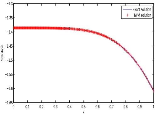
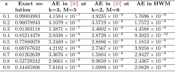
the exact solution isy(x) =e−x2. We solve this equation by the present method with k= 1 andM = 10. The numerical solutions of Eq. (5.9) are presented and compared with the exact solution and other existing method solutions in Table 3. Figure 4 rep-resents the physical interpretation of approximate solution with analytical solution of Eq. (5.9).
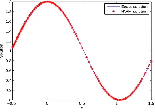
Example 5.5. Consider the scalar problem discussed in [1],
y′′(x) + (2 x)y
′(x) =−n2cos(nx)−2
Figure 3. Graphical representation of absolute error obtained by
HWM solution with exact solution for Example 5.3 atk= 1,M = 10 for different values of r.
0.1 0.2 0.3 0.4 0.5 0.6 0.7 0.8 0.9
3.8 3.9 4 4.1 4.2
4.3x 10
−5
x
Error analysis
Error at k=1, M=10 and r=0.25 Error at k=1, M=10 and r=0.75
Table 3. AE of HWM (at k = 1, M = 10) and Laguerre wavelet
method (LWM) [30] for different values ofkandM with exact solu-tion for the Example 5.4.
x Exact so-lution
AE in [30] at k=3, M=5
AE in [30] at k=2, M=6
AE in HWM
0.1 0.99004983 4.1584×10⁻⁷ 3.9235×10⁻⁸ 5.7696×10⁻⁹ 0.2 0.96078943 4.1079×10⁻⁷ 3.5719×10⁻⁸ 1.7572×10⁻⁸
0.3 0.91393118 1.3871×10⁻⁷ 3.4602×10⁻⁸ 4.4588×10⁻⁸ 0.4 0.85214378 2.0338×10⁻⁸ 2.8729×10⁻⁸ 9.2022×10⁻¹⁰
0.5 0.77880078 5.2489×10⁻⁸ 2.8886×10⁻⁸ 1.1813×10⁻⁸ 0.6 0.69767632 4.2192×10⁻⁸ 2.7567×10⁻⁸ 3.9258×10⁻⁸
0.7 0.61262639 3.3676×10⁻⁸ 1.5804×10⁻⁸ 2.9427×10⁻⁸
0.8 0.52729242 2.0661×10⁻⁸ 9.9659×10⁻⁹ 2.4367×10⁻⁸
0.9 0.44485806 7.6164×10⁻⁹ 1.0989×10⁻⁸ 2.0828×10⁻⁸
subjected to the initial conditions,
y(0) = 2, y′(0) = 0,
Figure 4. Physical interpretation of HWM solution with exact
so-lution for Example 5.4 atk= 1 and M = 10.
0 0.2 0.4 0.6 0.8 1
0.4 0.5 0.6 0.7 0.8 0.9 1 1.1
x
Solution
Exact solution HWM solution
Table 4. AE of the HWM solution with exact solution for the
Ex-ample 5.5.
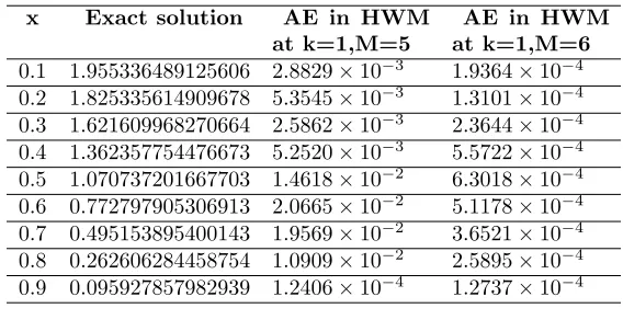
x Exact solution AE in HWM at k=1,M=5
AE in HWM at k=1,M=6 0.1 1.955336489125606 2.8829×10⁻³ 1.9364×10⁻⁴
0.2 1.825335614909678 5.3545×10⁻³ 1.3101×10⁻⁴
0.3 1.621609968270664 2.5862×10⁻³ 2.3644×10⁻⁴
0.4 1.362357754476673 5.2520×10⁻³ 5.5722×10⁻⁴
0.5 1.070737201667703 1.4618×10⁻² 6.3018×10⁻⁴
0.6 0.772797905306913 2.0665×10⁻² 5.1178×10⁻⁴ 0.7 0.495153895400143 1.9569×10⁻² 3.6521×10⁻⁴
0.8 0.262606284458754 1.0909×10⁻² 2.5895×10⁻⁴ 0.9 0.095927857982939 1.2406×10⁻⁴ 1.2737×10⁻⁴
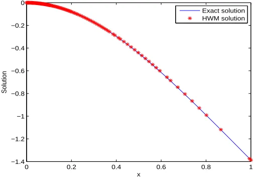
Example 5.6. Consider the following nonlinear Lane-Emden equation [30];
y′′(x) + 2 xy
′(x) + 4(2ey(x)+ey(2x)) = 0, 0< x <1, (5.11)
subjected to the initial conditions
y(0) = 0, y′(0) = 0,
Figure 5. Graphical representation of HWM solution and exact
so-lution for Example 5.5 atk= 1 and M = 10.
−0.50 0 0.5 1 1.5
0.2 0.4 0.6 0.8 1 1.2 1.4 1.6 1.8 2
x
Solution
Exact solution HWM solution
Table 5. AE of HWM, BPOM and Laguerre wavelet method (LWM) for different values of k and M with exact solution for the Example 5.6.
x Exact solu-tion
AE by BPOM at k=1, M=5 [4].
AE by LWM at k=2, M=7 [30].
AE by LWM at k=3,M=7 [30].
AE by HWM at k=1, M=10. 0.1 -0.01990066 2.0×10⁻⁵ 9.0×10⁻⁹ 4.5×10⁻¹² 3.6×10⁻¹¹ 0.2 -0.07844142 2.4×10⁻⁵ 1.6×10⁻⁹ 2.4×10⁻¹¹ 3.4×10⁻¹¹
0.3 -0.17235532 2.4×10⁻⁵ 6.3×10⁻⁹ 5.3×10⁻¹⁰ 3.6×10⁻¹¹
0.4 -0.29684001 1.8×10⁻⁵ 9.3×10⁻⁹ 1.1×10⁻⁹ 3.4×10⁻¹¹ 0.5 -0.44628710 2.4×10⁻⁵ 1.7×10⁻¹⁰ 1.4×10⁻⁹ 3.2×10⁻¹¹
0.6 -0.61496939 2.9×10⁻⁵ 1.7×10⁻⁷ 1.7×10⁻⁹ 3.3×10⁻¹¹
0.7 -0.79755223 2.5×10⁻⁴ 2.9×10⁻⁷ 1.8×10⁻⁹ 3.2×10⁻¹¹ 0.8 -0.98939248 1.4×10⁻⁴ 3.6×10⁻⁷ 1.6×10⁻⁹ 2.9×10⁻¹¹
0.9 -1.18665369 8.6×10⁻³ 4.1×10⁻⁷ 1.3×10⁻⁹ 2.8×10⁻¹¹
Figure 6 represents physical interpretation of approximate and exact solution for the Eq. (5.11).
Example 5.7. Consider the initial value problem [12],
Figure 6. Graphical representation of HWM solution and exact
so-lution for Example 5.6 atk= 1 and M = 10.
0 0.2 0.4 0.6 0.8 1
−1.4 −1.2 −1 −0.8 −0.6 −0.4 −0.2 0
x
Solution
Exact solution HWM solution
subjected to the initial conditions
y(0) = 0, y′(0) = 0,
the exact solution is y(x) = −2 ln(cosx). Here, solving Eq. (5.12) using Hermite wavelets collocation method and comparison between the Numerical solution, exact solution and other existed method solutions can be observed in Table 6. Figure 7 represents the comparison between the approximate solution and analytical solution graphically.
Example 5.8. Consider the oxygen diffusion problem [30],
y′′(x) + 2 xy
′(x) = 0.76129y(x)
y(x) + 0.03119, 0< x <1, (5.13)
subjected to the boundary conditions
y′(0) = 0, 5y(1) +y′(1) = 5,
where exact solution is unknown. Now we solve this equation by present method withk= 1 and different values of M. These solutions are in good agreement with the method in [11] and this results are tabulated in Table 7. As increasingM gives rise to better approximate solution, it can be seen from Table 7. Figure 8 shows absolute error between solution obtained by present method and method in [30].
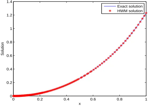
Example 5.9. Consider the initial value problem [7],
Table 6. AE of HWM, PIA and Legendre wavelet method (LWM)
with exact solution for the Example 5.7.
x Exact solution AE in PIA(1,3) algorithm [12]
AE in Legendre wavelet[1]
AE in HWM at k=1,M=10
0.1 0.010016711246471 6.71×10⁻⁶ 9.00×10⁻⁸ 9.88×10⁻⁷ 0.2 0.040269546104817 9.55×10⁻⁶ 1.50×10⁻⁷ 1.41×10⁻⁶
0.3 0.091383311852116 3.11×10⁻⁶ 6.14×10⁻⁷ 3.15×10⁻⁶ 0.4 0.164458038150111 8.04×10⁻⁶ 8.88×10⁻⁶ 3.70×10⁻⁶ 0.5 0.261168480887445 8.48×10⁻⁶ 5.67×10⁻⁵ 3.96×10⁻⁶
0.6 0.383930338838875 2.03×10⁻⁵ 2.55×10⁻⁴ 6.10×10⁻⁶ 0.7 0.536171515135862 7.15×10⁻⁵ 9.24×10⁻⁴ 7.84×10⁻⁶ 0.8 0.722781493622688 2.91×10⁻⁴ 2.90×10⁻³ 8.02×10⁻⁶
0.9 0.950884887171629 1.05×10⁻³ 7.90×10⁻³ 1.10×10⁻⁵
Figure 7. Graphical representation of HWM solution and exact
so-lution for Example 5.7 atk= 1 and M = 10.
0 0.2 0.4 0.6 0.8 1
0 0.2 0.4 0.6 0.8 1 1.2 1.4
x
Solution
Exact solution HWM solution
subjected to the initial condition
y(0) = 0,
Table 7. Numerical comparison between the HWM solution with
the method in [11] for the Example 5.8.
X Method in [30]
Present method at k=1, M=5
Present method at k=1, M=6
Present method at k=1, M=7 0.1 0.8297060924 0.8297056673 0.8297060849 0.8297060920 0.2 0.8333747335 0.8333742707 0.8333747242 0.8333747334 0.3 0.8394899139 0.8394894941 0.8394898940 0.8394899138 0.4 0.8480527849 0.8480524878 0.8480527556 0.8480527850 0.5 0.8590649271 0.8590647777 0.8590648972 0.8590649272 0.6 0.8725283199 0.8725282654 0.8725282986 0.8725283197 0.7 0.8884453056 0.8884452280 0.8884452950 0.8884453055 0.8 0.9068185480 0.9068183182 0.9068185410 0.9068185481 0.9 0.9276509883 0.9276505645 0.9276509744 0.9276509882
Figure 8. Graphical representation of absolute error by HWM
so-lution with soso-lution by [30] for Example 5.8 atk= 1 andM = 5,6,7.
0.1
0.2
0.3
0.4
0.5
0.6
0.7
0.8
0.9
−2
0
2
4
6
x 10
−7
x
Error analysis
Error at k=1, M=5
Error at k=1, M=6
Error at k=1, M=7
be observed in Table 8. Figure 9 represents the comparison between the approxi-mate solutions of HWM, ADM and analytical solution graphically. On solving above equation by ADM we obtain:
y1(x) = −x
2
2 ,
y2(x) = x
4
8,
y3(x) =−x
6
24,
Table 8. AE of HWM and ADM with exact solution for the
Exam-ple 5.9.
x Exact solution AE by ADM Y4
AE by ADM Y5
AE in HWM at k=1, M=10
0.1 -0.004987541511039 6.22×10⁻¹³ 2.69×10⁻¹⁵ 9.56×10⁻¹¹ 0.2 -0.019802627296180 6.29×10⁻¹⁰ 1.04×10⁻¹¹ 1.31×10⁻⁵ 0.3 -0.044016885416774 3.55×10⁻⁸ 1.33×10⁻⁹ 2.17×10⁻⁹ 0.4 -0.076961041136128 6.14×10⁻⁷ 4.08×10⁻⁸ 3.20×10⁻⁹ 0.5 -0.117783035656383 5.52×10⁻⁶ 5.74×10⁻⁷ 1.34×10⁻⁸ 0.6 -0.165514438477573 3.28×10⁻⁵ 4.91×10⁻⁶ 1.17×10⁻⁹ 0.7 -0.219135529916671 1.46×10⁻⁴ 2.98×10⁻⁵ 1.04×10⁻⁹ 0.8 -0.277631736598280 5.30×10⁻⁴ 1.40×10⁻⁴ 3.75×10⁻⁸ 0.9 -0.340037302785709 1.63×10⁻³ 5.46×10⁻⁴ 5.47×10⁻⁸
yn(x) = (−1)n (x2)n
n2n .
Then solution by ADM is,
y(x) =Y3(x) =−x
2
2 +
x4 8 −
x6 24,
y(x) =Y5(x) =−x
2
2 +
x4 8 −
x6 24+
x8 64 −
x10 160.
Figure 9. Graphical comparison between the HWM (atk= 1 and
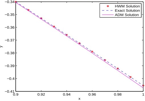
M = 10), ADMY5 with exact solution for Example 5.9.
0.9 0.92 0.94 0.96 0.98 1 −0.41
−0.4 −0.39 −0.38 −0.37 −0.36 −0.35 −0.34
x
y
Figure 10. Graphical representation of AE by HWM (atk= 1 and
M = 10), ADMY3, Y5 with exact solution for Example 5.9.
0 0.2 0.4 0.6 0.8 1
0 0.002 0.004 0.006 0.008 0.01 0.012
x
y
AE by HWM AE by ADM Y3 AE byADM Y5
Table 9. Comparison between the HWM and HM with exact
solu-tion for the Example 5.10.
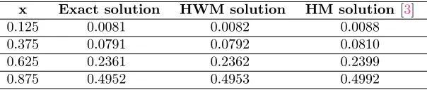
x Exact solution HWM solution HM solution [3] 0.125 0.0081 0.0082 0.0088 0.375 0.0791 0.0792 0.0810 0.625 0.2361 0.2362 0.2399 0.875 0.4952 0.4953 0.4992
Example 5.10. Consider the initial value problem [3],
y′(x) +y(x) =ex, 0< x <1, (5.15)
subjected to the initial condition
y(0) = 0, y′(0) = 0,
the exact solution isy(x) = 12(ex−sinx−cosx). Here, we solved Eq. (5.15) using Hermite wavelets collocation method and Haar wavelet method (HM). Comparison between the numerical, exact and adomian decomposition method solutions can be observed in Table 9.
6. Conclusion
are presented in Tables and Figures in comparison with the exact solutions. HWM solutions are quite satisfactory in comparison with the existing numerical solutions available in the literature [1,3,4,12, 13,24, 30]. This scheme is easy to implement with computer programs and it can be extend for higher order with slight modifica-tion. Proposed Theorem 3.1 reveals that the present method will contribute exact solution for differential equations, whose solutions are in the form of polynomials of finite degree. This is important for the development of new research in the field of numerical analysis and beneficial for new researchers. Also, Theorems 3.2 and 3.3 on uniform convergence and error analysis.
Acknowledgment
It is a pleasure to thank the University Grants Commission (UGC), Govt. of India for the financial support under UGC-SAP DRS-III for 2016-2021:F.510/3/DRS-III/2016(SAP-I) Dated: 29th Feb. 2016.
References
[1] Y. Aksoy and M. Pakdemirli,New perturbation iteration solutions for Bratu type equations, Comput. Math. Appl.,59(8) (2010), 2802–2808.
[2] A. Ali, M. A. Iqbal, and S. T. Mohyud-Din, Hermites wavelets method for Boundary Value problems, International Journal of Modern Applied Physics,3(1) (2013), 38–47.
[3] S. Arora, Y. S. Brar, and S. Kumar, Haar Wavelet Matrices for the Numerical Solutions of Differential Equations, International Journal of Computer Applications,97(2011), 1–4. [4] B. Basirat, and M. A. Shahdadi,Application of the BPOM for numerical solution of the
isother-mal gas spheres equations, International Journal of Research and Reviews in Applied Sciences,
18(1) (2014), 85–94.
[5] E. H. Doha, W. M. Abd-Elhameed, and Y. H. Youssri,New ultraspherical wavelet collocation method for solving 2nth order initial and boundary value problem, Journal of the Egyptian
Mathematical Society,24(2) (2016), 319–327.
[6] V. S. Erturk, Differential transformation method for solving differential equations of Lanr-Emden type, Mathematical and Computational Applications,12(3) (2007), 135–139.
[7] M. Hermann and M. Saravi,Nonlinear ordinary differential equations, Springer, India, 2016. [8] R. Jiwari, A hybrid numerical scheme for the numerical solution of the Burgers’ equation,
Computer Physics Communications,188(2015), 59–69.
[9] R. Jiwari,Haar wavelet quasilinearization approach for numerical simulation of Burgers’ equa-tion, Computer Physics Communications,183(2012), 2413–2423.
[10] R. Jiwari and R. C. Mittal,A Numerical Scheme for singularly perturbed Burger-Huxley Equa-tion, J. Appl. Math.,29(2011), 813–829.
[11] M. Kumar and N. Singh,A collection of computational techniques for solving singular boundary value problems, Adv. Eng. Softw.,40(2009), 288–297.
[12] S. Liao and Y. Tan, A general approach to obtain series solutions of nonlinear differential equations, Stud. Appl. Math.,119(4) (2007), 297–354.
[13] T. Lot and K. Mahdiani, Numerical solution of boundary value problem by using wavelet-galerkin method, Mathematical Science,1(2007), 07–18.
[14] A. K. Nasab, A. Kilicman, E. Babolian, and Z. P. Atabakan,Wavelet analysis method for solving linear and nonlinear singular boundary value problems, Applied Mathematical Modelling,37(8) (2013), 5876–5886.
[16] R. Rajaraman and G. Haiharan,An efficient wavelet based spectral method to singular boundary value problems, Journal of Math Chem,53(9) (2015), 2095–2113.
[17] M. N. Sahlan and E. Hashemizadeh,Wavelet Galerkin method for solving nonlinear singular boundary value problems arising in physiology, Applied Mathematical Computation,250(2015), 260–269.
[18] S. C. Shiralashetti and A. B. Deshi,An efficient Haar wavelet collocation method for the numer-ical solution of multi-term fractional differential equations, Nonlinear Dyn.,83(2016), 293–303. [19] S. C. Shiralashetti, A. B. Deshi, and P. B. Mutalik Desai,Haar wavelet collocation method for the numerical solution of singular initial value problems, Ain. Shams. Engg. J.,7(2) (2016), 663–670.
[20] S. C. Shiralashetti and S. Kumbinarasaiah, Laguerre wavelets collocation method for the nu-merical solution of the Benjamina-Bona-Mohany equations, Journal of Taibah University for Science, 2018. DOI 10.1080/16583655.2018.1515324.
[21] S. C. Shiralashetti and S. Kumbinarasaiah,Hermite wavelets operational matrix of integration for the numerical solution of nonlinear singular initial value problems, Alexandria Engineering Journal, 2017. DOI 10.1016/j.aej.2017.07.014.
[22] S. C. Shiralashetti and S. Kumbinarasaiah,Theoretical study on continuous polynomial wavelet bases through wavelet series collocation method for nonlinear lane-Emden type equations, Ap-plied Mathematics and Computation,315(2017), 591–602.
[23] S. C. Shiralashetti and S. Kumbinarasaiah,Cardinal B-spline wavelet based numerical method for the solution of generalized burgers-huxley equation, International journal of applied and computational mathematics, 2018. DOI 10.1007/s40819-018-0505-y.
[24] S. Upadhyay, S. Singh, S. Yadav, and N. K. Rai,Numerical solution of two point boundary value problems by using wavelet-galerkin method, International Journal of Applied Mathematical Research,4(4) (2015), 496–512.
[25] M. Usman, and S. T. Mohyud-Din,Physicists Hermites wavelets method for singular differential equation, International Journal of Advances in Applied Mathematics and Mechanics,1(2) (2013), 16-29.
[26] S. G. Venkatesh, S. K. Ayyaswamy, and S. R. Balachandar,Legendre wavelet method for solving initial problem of Bratu-type, Computers and Mathematics with Applications, 63(8) (2012), 1287–1295.
[27] A. M. Wazwaz,A new method for solving singular initial value problem in the second order ordinary differential equations. Applied Mathematical and Computation,128(2002), 45–57. [28] C. Yang and J. Hou,Chebyshev wavelets method for solving Bratu’s problem, Boundary Value
Problems,142(2013), 01–09.
[29] S. A. Yousefi,Legendre wavelet method for solving differential equation of Lane-Embden type, Applied Mathematics and Computations,181(2) (2006), 1417–1422.
![Table 1. Comparison of the absolute error (AE) of HWM (presentmethod at k = 1, M = 10), wavelet Galerkin method by Coiflet[13] and Legendre wavelet Galerkin method (LWGM) [24] with exactsolution for the Example 5.1.](https://thumb-us.123doks.com/thumbv2/123dok_us/8943338.1852706/8.612.185.425.470.649/comparison-absolute-presentmethod-galerkin-coiet-legendre-galerkin-exactsolution.webp)
![Table 7. Numerical comparison between the HWM solution withthe method in [11] for the Example 5.8.](https://thumb-us.123doks.com/thumbv2/123dok_us/8943338.1852706/18.612.185.426.354.539/table-numerical-comparison-hwm-solution-withthe-method-example.webp)