in the population sciences published by the Max Planck Institute for Demographic Research Doberaner Strasse 114 · D-18057 Rostock · GERMANY www.demographic-research.org
DEMOGRAPHIC RESEARCH
VOLUME 7, ARTICLE 16, PAGES 537-564
PUBLISHED 29 NOVEMBER 2002
www.demographic-research.org/Volumes/Vol7/16/
DOI: 10.4054/DemRes.2002.7.16
Research Article
Socioeconomic Differentials in Divorce
Risk by Duration of Marriage
Marika Jalovaara
1 Introduction 538
2 Individual time and divorce 539
3 Interactions between spouses’ socioeconomic position and the duration of marriage
540
4 Purpose of the study 542
5 Data and methods 543
5.1 Data set 543
5.2 Duration of marriage 544
5.3 Measurement of socioeconomic position 544
5.4 Control variables 545
5.5 Methods 546
6 Results 548
6.1 Distributions of marriage-years 548
6.2 Duration of marriage and divorce risk 550 6.3 Socioeconomic differentials in divorce risk by
duration of marriage
550
7 Discussion 556
Acknowledgements 559
Notes 560
Research Article
Socioeconomic Differentials in Divorce Risk by Duration of
Marriage
Marika Jalovaara1
Abstract
Using register-based data on Finnish first marriages that were intact at the end of 1990 (about 2.1 million marriage-years) and followed up for divorce in 1991–1993 (n = 21,204), this research explored the possibility that the effect of spouses’ socioeconomic position on divorce risk varies according to duration of marriage. The comparatively high divorce risks for spouses with little formal education and for spouses in manual worker occupations were found to be specific to marriages of relatively short duration. In contrast, such factors as unemployment, wife’s high income, and living in a rented dwelling were found to increase divorce risk at all marital durations.
1
1. Introduction
As divorce has become common in almost all Western countries, many social scientists are attempting to understand the factors that hold marriages together or contribute to divorce. Micro-level research has related divorce to various demographic, socioeconomic, and social-psychological factors (for a review, see White 1990).
Research findings on micro-level determinants of divorce are frequently interpreted using versions of the social exchange theory. Levinger’s (1976) framework distinguishes three categories of factors that individuals presumably assess when considering divorce: the attraction to the ongoing marriage, barriers to breaking up the marriage, and alternatives to the current marriage. The economic theory of marital instability (Becker, Landes, and Michael 1977) provides a similar but more formal rational choice framework.
The other influential theoretical approach guiding research on antecedents of divorce is the life course perspective (Aldous 1990, Bengtson and Allen 1993). With its attention to the timing and sequencing of events in the lives of individuals and families, the life course perspective has increased the awareness of the potential time-dependency of divorce determinants, that is, the possibility that the antecedents of divorce vary with individual (and historical) time (White 1990, p. 909). The possibility that divorce determinants interact with individual time is highly plausible: The significance of marriage as well as the consequences of divorce for the individuals involved presumably vary over the various stages of marital lives, and antecedents of divorce can be expected to vary accordingly (South and Spitze 1986). In order to gain a better understanding of divorce, it is essential to know whether the empirical research and the exchange-based theoretical models concerning the determinants of divorce need specification in order to take the variation of divorce determinants over life course into account.
socioeconomic determinants of divorce in midlife and later life. (If these interactions are ignored, the understanding of the effects of socioeconomic factors on the risk of divorce remains overwhelmingly restricted to relatively short durations of marriage, where the incidence of divorce is highest.) In analyses of socioeconomic determinants of divorce and separation, the duration of marriage and the ages of spouses are standard control variables, but their interactions with socioeconomic factors have been examined in relatively few recent studies (Booth, Johnson, White, and Edwards 1986, Morgan and Rindfuss 1985, South 2001, South and Spitze 1986, White and Booth 1991. All of these use survey material from the United States). This research extends previous knowledge by using data from Finland, a Northern European country; by using a data set that is very extensive in size; by including a comparatively wide range of marital durations (up to 39 years); and by using several indicators of the socioeconomic position of both partners.
2. Individual time and divorce
The major challenge in analyses concerning temporal determinants of divorce is that the various dimensions of historical time and individual time are highly related and therefore, it is difficult to disentangle the independent effect of each of them in a meaningful way (see Thornton and Rodgers 1987). The main trends and differences are, however, clear. From the end of the 19th century, the Western world has experienced a rise in divorce, accelerating since the 1960s. Successive cohorts and new periods have presented higher rates of divorce than their predecessors (Haskey 1993, Lutz, Wils, and Nieminen 1991, Phillips 1991, pp. 185−223, Pitkänen 1986, Thornton and Rodgers 1987). In some countries, including the United States, divorce rates during the recent decades have leveled off at their historical highs or have even declined (Goldstein 1999). On the other hand, individual time has been reported to be inversely related to the likelihood of divorce and separation. Divorce and separation are less likely when the spouses are older, when the spouses have married at a higher age, and when the marriages have lasted a longer time (Morgan and Rindfuss 1985, South and Spitze 1986, Thornton and Rodgers 1987).
stability may be partly specific to the generation rather than the duration of marriage or the ages of spouses (White and Booth 1991, p. 6).
Moreover, there are theoretical reasons to expect that the actual propensity to divorce declines as spouses age and marriages last longer. Social-psychological explanations suggest that older people are socially and emotionally more mature and personally stable and therefore more able to avoid or solve serious marital conflicts than younger people; that older spouses are less likely undergo rapid individual changes and this limits the chances that the expectations and views of the two spouses will diverge (Morgan and Rindfuss 1985, Thornton and Rodgers 1987); and that older people put a higher value on stability than young people (Booth et al. 1986). The social exchange theory posits that older spouses have fewer alternatives to their current relationship, and because they have less time to enjoy any benefits that might follow from divorce, the expected future benefits compare less favorably with the costs of divorce (Ross and Sawhill 1975, p. 40). Also, the costs of divorce should be higher for couples that have been together for a longer time, because over time they tend to have made many tangible as well as intangible marital-specific investments (Becker et al. 1977) that act as barriers to divorce. A higher attraction to the current marriage is usually not considered a cause for the lower divorce risk at high marital durations. Indeed, recent research from the United States suggests that self-reported marital happiness tends to decline over the marital life course. (Whether there is a slight upturn in later years is under debate; see VanLaningham, Johnson, and Amato 2001).
3.
Interactions between spouses’ socioeconomic position and the
duration of marriage
socioeconomic status of spouses (such as occupational class, income, and home-ownership) should become more indicative of the spouses’ lifetime economic success (Booth et al. 1986, South and Spitze 1986). Also, at higher ages and marital durations, it may be more difficult for the spouses to accept economic insecurity and any accompanying difficulties as just a temporary state of affairs.
On the other hand, there are reasons to expect that socioeconomic differentials in the risk of divorce diminish with time in the marriage. Firstly, it could be expected that having few economic resources is less predictive of divorce at longer durations of marriage, because the couples tend to have built up various kinds of barriers to leaving the relationship. For instance, they have a long shared history, and they often have shared children and social networks, and such barriers may help maintain the marital bond through times of economic difficulties. Secondly, the fact that the spouses have, for instance, stable employment, high occupational status, and some material assets early in marriage may be taken to indicate that they are well-prepared for assuming responsibility for a family. The proper preparation is presumed to strengthen the conjugal relationship especially at its early stages, since in later years, current developments within the marriage should play an increasingly important role (see South and Spitze 1986). Thirdly, especially at later stages of individual and marital life courses, greater social and economic resources might also widen the array of attractive alternatives to remaining married, should the marriage turn out unsatisfying. For instance, it has been suggested that especially later in marriage, highly educated women are more likely to find alternative partners and to be economically independent, and therefore, they might later in marriage be equally (or even more) divorce-prone than less educated women (South and Spitze 1986).
4. Purpose of the study
The present study aims at contributing to the understanding of socioeconomic differentials in divorce risk by exploring the possibility that the effect of the socioeconomic position of the spouses varies with the duration of marriage (that is, time elapsed in marriage). The study uses register-based data concerning Finnish first marriages that were intact at the end of 1990 and were followed up for divorce between 1991 and 1993. The analysis uses several indicators of the socioeconomic position of both the wife and the husband. Because of its differential distributions in the various birth cohorts, the level of spouses’ formal education may be a problematic measure of socioeconomic position. Consequently, a fuller picture of the interactions between socioeconomic and temporal factors can be gained when other measures of the socioeconomic position of the spouses are also used. The very extensive size of the data is an advantage when examining divorce determinants at longer marital durations where the incidence of divorce is low. In the present analysis, the highest observed marital duration is limited to (the comparably high figure of) 39 years.
Studies on marital dissolution are best conducted by observing successive marriage cohorts from the time they are initiated. The cohort approach is particularly advantageous when the analysis focuses on the effects of historical and individual time on marital stability. However, the present analysis is based on a left-truncated study population, meaning that the marriages were of varying durations at the beginning of the 3-year follow-up. In such data, the effects of the duration of marriage are confounded with the effects of membership in various birth and marriage cohorts, and it is not possible to unconfound the effects. In principle, any interaction between a socioeconomic factor and the duration of marriage could just as well be related to cohort as to the duration of marriage. The changes in socioeconomic differentials in divorce risk over the marital life course (which in the present analysis are represented synthetically) may be the interactions of greater theoretical importance. However, when interpreting the results of the present analysis, the possibility that the patterns are related to cohort also needs to be considered.
from 41 in 1990 to 51 in 1999; the TDR was 43 in 1991, 1992, and 1993, which are the follow-up years of this study (Statistics Finland 1992a, Statistics Finland 2001, p. 146).
5. Data and methods
5.1 Data set
The study uses tabulated data that are based on a census-linked divorce data file compiled at Statistics Finland (permission number TK-53-1016-98). The records of wives and husbands from the register-based 1990 census were linked to each other and with divorce records (as well as other annual records) for the years 1991–1993. Dates of divorce refer to the dates on which divorce is granted, information concerning which are transmitted to the Population Register Centre by district courts.
Neither the dissolution of consensual unions nor the time spent in premarital consensual unions are considered owing to data limitations. Finnäs (1995, 1996) has shown that by the beginning of the study period, living in a consensual union had become the typical way to begin a union in Finland. However, consensual unions tended to end in either judicial marriage or separation, meaning that cohabitation as a long-term alternative to formal marriage had not yet become common (Finnäs 1995, 1996). Still, it is obvious that the exclusion of consensual unions and their dissolution lead to a partial picture of union dissolution in Finland in the early 1990s.
The study includes judicial marriages that were intact on 31 December 1990, that were the first for both spouses, where both spouses were Finnish citizens, where the wife’s age was below 65, and where the spouses were registered as domiciled in the same dwelling at the beginning of the follow-up. This analysis is further restricted to marriages that had lasted for less than 40 years. Among couples that have been married for 40 years or longer, the incidence of divorce is very low and therefore, the results would be neither reliable nor very interesting. Also, the measurement of the socioeconomic position of the oldest spouses would be somewhat problematic because the oldest spouses tend to have retired from work.
The same data have been used in two previous studies concerning the effects of the socioeconomic position of spouses on the risk of divorce (Jalovaara 2001, in press). The only difference between the study populations followed up in these studies is that in the two previous studies, marriages that had lasted for 40 years or longer were also included.
were dropped and ceased to contribute marriage-years on the dates of divorce, wife’s or husband’s death, wife’s emigration, the 40th anniversary of the wedding, or at the end of the follow-up period, whichever came first. After all restrictions, the data included about 2.10 million marriage-years at risk, and during the follow-up period 21,204 marriages were dissolved through divorce.
5.2 Duration of marriage
Marital duration, that is, time elapsed since the day of marriage, was used as the life course measure. The value of the variable changed at the anniversary of the wedding if the marriage reached the subsequent category of marital duration. In order to examine whether – and how – the effects of socioeconomic factors varied with the duration of marriage, the couples were divided into five categories of marital duration. These categories are less than 5 years, 5 to 9 years, 10 to 19 years, 20 to 29 years, and 30 to 39 years. Note that the first two categories are five-year categories, whereas the rest are 10-year categories. In preliminary analyses, 5-10-year categories were used also at higher marital durations, but this more detailed classification did not prove informative.
5.3 Measurement of socioeconomic position
The socioeconomic position of the spouses was depicted with respect to each spouse’s level of education, occupational class, economic activity, and income, as well as the couple’s housing tenure and housing density. Each variable describes the circumstances of the spouses at the beginning of the study period, that is, at the end of 1990.
Wives’ and husbands’ education refers to the highest educational qualification the person had achieved by the end of 1990. The data were obtained from the Statistics Finland’s register of completed degrees. Here, four educational levels were distinguished: (a) Basic (about 9 years or less; persons for whom no data on post-basic education is registered); (b) Lower secondary (persons with an occupational training of less than 3 years); (c) Upper secondary (persons with an occupational training of 3 years, as well as persons who have a completed matriculation examination), and (d) Tertiary (persons with an occupational training of 4–5 years, or a university-level certificate or degree).
pensioners, persons performing domestic work etc.) were classified as far as possible on the basis of their occupation in 1985 or 1980. Husbands and wives for whom neither current nor previous occupation was found, were classified whenever possible under the same occupational class as the head of the household. The exception consists of students, for whom neither earlier occupation nor occupation of head of household were searched; all students are in the group “other”.
The variables concerning wives’ and husbands’ economic activity were based on Statistics Finland’s classification of the “main type of activity”. This, in turn, was based on data obtained from various registers on a person’s economic activity during the 1990 census week from December 25th to 31st. The categories are as follows: employed (comprising wage earners and entrepreneurs), unemployed (persons registered as actively seeking work), students (here including conscripts and conscientious objectors), pensioners, and the residual category of others outside the labor force. This last category (“others”) comprises persons performing domestic work full-time (who usually are women).
The data on wife’s and husband’s income originate from the tax files of the national taxation registers, and the income variables describe the level of the person’s income subject to state taxation in 1990. Five income categories are distinguished (see Table 2).
Housing tenure was measured in three classes: home-owner, rented, and unknown.
Statistics Finland’s housing density classification divides household-dwelling units into spacious, normal, and overcrowded (as well as unknown) by comparing the number of persons in the unit and the number of rooms in the dwelling (kitchen excluded). If there was more than one person per room, the dwelling was classified as overcrowded. The dwelling was classified as spacious if there were at least five rooms for two persons, at least six rooms for three persons, at least seven rooms for four persons, or at least eight rooms for five persons (Statistics Finland 1992b, pp. 15–16.).
5.4 Control variables
Four control variables were included in all models because they were likely to affect both the socioeconomic position of spouses (at the end of 1990) and the risk of divorce (in 1991−93). The wife’s age at marriage was calculated exactly on the basis of the date of birth and the date of entry into marriage, and then grouped into 5-year categories.
Wife’s age was measured at the beginning of the follow-up (at the end of 1990), and was
residing in the same household as the married couple at the end of 1990. The last control variable was the degree of urbanization of the municipality of the couple’s residence at the end of 1990. This last variable was based on Statistics Finland’s classification. Here, the capital city region (here including Helsinki, Espoo, Vantaa, and Kauniainen) was treated as a separate category.
5.5 Methods
The data were cross-tabulated according to the variables included in the analysis. Each cell of the cross-tabulation includes information on the number of divorces granted and the marriage-years lived in 1991−1993. The table was analyzed by means of Poisson regression. All explanatory variables were treated as categorical. In the model it is assumed that the expected divorce rate (the ratio of divorce events to exposure time) in a certain combination i of the explanatory variables can be described by the equation:
E(d
i)/(Vi) = exp(a + b1x1i + b2x2i + …+bpxpi),
where
E
(di) is the expected number of divorces in the i
th cell, V
i is the number of
marriage-years lived in the ith cell, x
1i …xpi are the explanatory variables, and a, b1 …bp are the parameters to be estimated. The models were fitted with GLIM (Francis, Green, and Payne 1993). The results are presented as ‘relative divorce risks’ (rate ratios). The statistical significance of an added term was measured by means of scaled deviance, which is asymptotically
χ
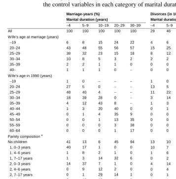
2-distributed. After testing the statistical significance of interactions between the duration of marriage and each socioeconomic variable, separate models describing the associations between the socioeconomic variables and the risk of divorce were fitted for each category of marital duration. 95% confidence intervals were calculated for the relative risks.Table 1: Marriage-years (%) and divorces (in 100s) in 1991−93 according to the control variables in each category of marital duration
Marriage-years (%) Divorces (in 100s) Marital duration (years) Marital duration (years)
−4 5−9 10−19 20−29 30−39 −4 5−9 10−19 20−29 30−39
All 100 100 100 100 100 29 46 77 50 10
Wife’s age at marriage (years)
−19 6 8 15 24 22 4 6 18 17 3
20−24 43 48 55 56 57 15 25 43 28 6
25−29 38 32 23 15 18 8 12 13 4 1
30−34 10 8 5 3 2 2 2 2 0 0
35−39 2 2 1 1 0 0 0 0 0 0
40− 1 1 1 0 − 0 0 0 0 −
Wife’s age in 1990 (years)
−19 1 0 − − − 1 0 − − −
20−24 27 5 0 − − 13 5 0 − −
25−29 48 40 4 − − 11 22 6 − −
30−34 18 39 28 0 − 3 14 28 0 −
35−39 4 12 43 8 − 1 3 31 8 −
40−44 1 3 20 40 0 0 1 10 25 0
45−49 0 1 4 35 9 0 0 1 14 2
50−54 0 0 1 13 35 0 0 0 3 5
55−59 0 0 0 3 38 0 0 0 0 2
60−64 0 0 0 1 17 0 0 0 0 1
Family composition a
No children 41 13 6 45 94 13 10 5 18 9
1, 0−3 years 40 17 1 0 0 10 7 1 0 0
1, 4−6 years 1 8 2 1 0 1 6 2 1 0
1, 7−17 years 1 3 14 32 6 0 2 14 18 1
2, 0−3 years 14 37 7 1 0 4 14 5 0 0
2, 4−6 years 0 9 12 2 0 0 4 11 1 0
2, 7−17 years 0 1 29 14 1 0 1 23 8 0
3+, 0−3 years 2 12 13 1 0 0 3 6 0 0
3+, 4−6 years 0 1 8 2 0 0 1 5 1 0
3+, 7−17 years 0 0 7 3 0 0 0 5 2 0
Degree of urbanization
Helsinki region 20 16 14 14 13 7 9 13 8 1
Other urban 43 40 39 41 40 14 21 34 23 5
Other densely populated 15 17 18 18 17 4 7 12 9 2
Rural 22 27 29 27 31 4 9 17 10 3
Total number of
marriage-years (in 1000s) 177 269 592 624 442
Divorces/1000 marriage-years 16.2 17.0 13.0 8.0 2.4
a
6. Results
6.1 Distributions of marriage-years
Table 1 shows the distributions of marriage-years (%) and divorces (in 100s) according to the control variables, separately for each of the five marital duration categories. It shows that the proportions of marriage-years contributed by couples wed at a young age were higher among marriages at longer durations. The wife’s age at the beginning of the follow-up is, of course, strongly and positively associated with the duration of marriage. The distributions of marriage-years by family composition indicate that couples in their first decade of marriage were typically at the childbearing stage, whereas couples in the third and fourth decade in marriage tended to have reached the post-parental stage. Finally, marriage-years contributed by couples living in rural areas increased with increasing duration of marriage.
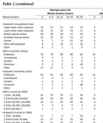
Table 2: Marriage-years (%) and divorces in 1991−93 (in 100s) according to the
indicators of socioeconomic position in each category of marital duration
Marriage-years (%) Divorces (in 100s) Marital duration (years) Marital duration (years)
−4 5−9 10−19 20−29 30−39 −4 5−9 10−19 20−29 30−39
All 100 100 100 100 100 29 46 77 50 10
Wife’s education
Basic or unknown 13 15 24 45 67 8 10 21 21 7
Lower secondary 25 31 34 30 20 8 15 27 16 2
Upper secondary 44 36 25 14 6 10 16 19 8 1
Tertiary 17 18 17 12 7 2 5 11 6 1
Husband’s education
Basic or unknown 18 20 28 45 64 9 11 24 21 6
Lower secondary 37 39 35 26 16 11 20 29 14 2
Upper secondary 27 22 18 13 9 7 10 13 7 1
Tertiary 17 19 19 16 11 2 5 11 8 1
Wife’s occupational class
Upper white collar employee 15 17 15 12 9 3 5 10 6 1
Lower white collar employee 46 45 47 44 34 12 21 38 24 4
Skilled manual worker 12 12 10 10 11 4 6 8 5 1
Unskilled manual worker 10 10 11 16 23 5 6 10 9 2
Farmer 4 6 7 10 14 0 1 2 2 1
Other self-employed 3 4 6 6 6 1 2 5 4 1
Table 2 (continued)
Marriage-years (%) Divorces (in 100s) Marital duration (years) Marital duration (years)
Marital duration −4 5−9 10−19 20−29 30−39 −4 5−9 10−19 20−29 30−39 Husband’s occupational class
Upper white collar employee 19 21 21 19 14 3 7 13 10 1
Lower white collar employee 22 21 19 19 17 6 9 15 10 2
Skilled manual worker 28 28 28 27 26 9 15 24 14 3
Unskilled manual worker 15 13 12 13 14 6 8 12 6 2
Farmer 5 7 8 10 14 0 1 2 2 1
Other self-employed 6 8 10 11 10 2 5 10 7 1
Other 6 2 1 1 6 2 2 1 1 0
Wife’s economic activity
Employed 75 76 85 88 65 20 35 66 44 8
Unemployed 3 3 2 2 3 1 2 3 2 0
Student 8 4 3 1 0 3 3 3 1 0
Pensioner 0 1 1 4 26 0 0 1 2 2
Other 14 17 9 4 6 4 6 4 2 0
Husband’s economic activity
Employed 90 94 94 89 58 24 41 69 44 7
Unemployed 4 3 3 2 2 2 3 4 2 0
Student 4 2 1 0 0 2 1 1 0 0
Pensioner 1 1 2 7 39 0 1 2 3 3
Other 1 1 1 1 1 1 1 1 1 0
Wife's income (in 1990)
1 (FIM −49,999) 24 25 20 17 34 9 12 13 7 3
2 (FIM 50,000−99,999) 58 54 50 49 46 16 25 41 25 5
3 (FIM 100,000−149,999) 15 17 23 26 16 3 7 18 13 2
4 (FIM 150,000−199 999) 2 3 4 5 3 0 1 3 3 0
5 (FIM 200,000−) 1 1 2 2 1 0 0 2 1 0
Husband's income (in 1990)
1 (FIM −49,999) 11 7 6 7 15 4 5 7 4 1
2 (FIM 50,000−99,999) 33 27 21 21 36 11 14 18 10 3
3 (FIM 100,000−149,999) 39 41 40 37 27 10 19 30 18 3
4 (FIM 150,000−199 999) 12 16 18 18 11 2 6 13 10 1
5 (FIM 200,000−) 6 9 15 17 10 1 3 9 8 1
Housing tenure
Home owner 63 79 88 91 92 14 30 61 43 9
Rented 35 20 11 8 8 15 15 15 7 1
Unknown 2 1 1 0 0 0 1 1 0 0
Housing density
Spacious 20 15 12 32 62 4 7 9 14 6
Normal 65 67 73 60 32 20 30 55 31 4
Overcrowded 13 17 13 7 4 5 8 11 4 0
Table 2 shows the distribution of marriage-years (%) and divorces (in 100s) by each socioeconomic variable, separately for each category of marital duration. Reflecting the increase in education over birth cohorts, women and men at shorter marital durations tended to have reached higher levels of education than women and men at higher marital durations. As for occupational class, the most significant difference in distributions between the categories of marital duration is that the proportion of marriage-years contributed by farmers increased towards spouses at higher marital duration, who tended to be members of earlier birth and marriage cohorts.
Table 2 also shows that the proportion of marriage-years contributed by couples with employed wives is highest among couples in their second and third decade of marriage. A number of young spouses were still in education. Moreover, during the early years in marriage, some women leave the labor force because they have young children. Note, however, that in later stages of family careers, married women tended to belong to the labor force in equal proportions with their husbands. The proportion of marriage-years contributed by pensioners was highest at high marital durations. Further, women and men tended to have highest incomes at medium durations of marriage. Finally, home-ownership became more prevalent towards higher marital durations and couples that had been married for a long time were likeliest to live in spacious dwellings.
6.2 Duration of marriage and divorce risk
The usual empirical pattern of divorce by the duration of marriage in Finland is that the divorce rate increases sharply during the first years in marriage and then, after having peaked, declines towards long marital durations (Lindgren and Ritamies 1994, Pitkänen 1986). The pattern was found also in these data (see bottom of Table 1). The risk of divorce was highest for marriages that had lasted 5–9 years and decreased thereafter, reaching a very low level at long marital durations. Note that in this study design, the marriages of shorter durations represented more recent marriage cohorts. Therefore, the higher divorce risk for marriages at shorter durations of marriage during the period studied partly reflects the increase in divorce risk over marriage cohorts.
6.3 Socioeconomic differentials in divorce risk by duration of marriage
socioeconomic position was tested in a model including the main effects of marital duration, the four control variables, and all indicators of the socioeconomic position of spouses, as well as the interactions between each socioeconomic indicator and marital duration. In this model, all but one first order interactions between the socioeconomic indicators and marital duration were statistically significant at one per cent risk level. The one interaction that was not statistically significant was the interaction between husband’s occupational class and marital duration (p = .132). Note, however, that some of the interactions may be statistically significant because of the large number of observations in the data, and therefore, it is possible that the statistical significance of interactions is not a very useful tool in this case when singling out the interactions that are sizable enough to be important.
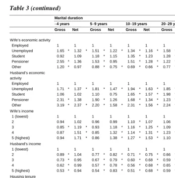
Table 3: Grossa and netb effects of socioeconomic factors in each category of
marital duration; relative divorce risks (rate ratios)
Marital duration
−4 years 5−9 years 10−19 years 20−29 years 30−39 years Gross Net Gross Net Gross Net Gross Net Gross Net
Wife’s education
Basic or unknown 1 1 1 1 1 1 1 1 1 1
Lower secondary 0.59 * 0.66 * 0.78 * 0.84 * 0.93 * 0.96 1.11 * 1.11 * 1.18 * 1.15 Upper secondary 0.39 * 0.50 * 0.65 * 0.74 * 0.88 * 0.93 1.16 * 1.14 * 1.21 1.17 Tertiary 0.29 * 0.40 * 0.45 * 0.54 * 0.82 * 0.83 * 1.10 1.01 1.08 0.99
Husband’s education
Basic or unknown 1 1 1 1 1 1 1 1 1 1
Lower secondary 0.67 * 0.78 * 0.90 * 0.97 0.95 1.00 1.06 1.06 1.12 1.13 Upper secondary 0.51 * 0.64 * 0.74 * 0.85 * 0.89 * 0.94 1.07 1.01 1.30 * 1.34 * Tertiary 0.30 * 0.41 * 0.48 * 0.59 * 0.71 * 0.79 * 1.04 0.98 0.95 1.01
Wife’s occupational class
Upper white collar emp. 1 1 1 1 1 1 1 1 1 1
Lower white collar emp. 1.37 * 0.96 1.35 * 0.96 1.06 0.91 * 0.94 0.92 0.91 0.78 Skilled manual worker 1.77 * 1.09 1.52 * 1.04 1.09 0.94 0.90 0.90 0.92 0.84 Unskilled manual worker 2.05 * 1.09 1.73 * 1.05 1.15 * 0.90 0.98 0.95 0.93 0.83 Farmer 0.52 * 0.59 * 0.46 * 0.45 * 0.43 * 0.44 * 0.40 * 0.51 * 0.54 * 0.50 * Other self-employed 2.30 * 1.40 * 1.78 * 1.18 1.18 * 1.02 1.05 0.99 1.36 * 1.15
Other 1.39 * 0.95 1.63 * 1.04 1.46 * 1.06 1.19 1.04 1.40 1.18
Husband’s occupational class
Upper white collar emp. 1 1 1 1 1 1 1 1 1 1
Lower white collar emp. 1.44 * 0.94 1.30 * 0.92 1.21 * 1.04 0.98 0.94 1.08 1.02 Skilled manual worker 1.70 * 0.87 1.53 * 0.92 1.21 * 0.96 0.96 0.91 1.00 1.02 Unskilled manual worker 2.16 * 0.99 1.74 * 1.00 1.46 * 1.12 0.98 0.92 1.21 1.25 Farmer 0.63 * 0.50 * 0.61 * 0.64 * 0.65 * 0.82 * 0.51 * 0.71 * 0.78 1.13 Other self-employed 2.05 * 1.08 1.92 * 1.18 * 1.48 * 1.18 * 1.19 * 1.09 1.46 * 1.40 *
Table 3 (continued)
Marital duration
−4 years 5−9 years 10−19 years 20−29 years 30−39 years Gross Net Gross Net Gross Net Gross Net Gross Net
Wife’s economic activity
Employed 1 1 1 1 1 1 1 1 1 1
Unemployed 1.65 * 1.32 * 1.51 * 1.22 * 1.34 * 1.16 * 1.58 * 1.43 * 1.13 1.11
Student 0.92 1.09 1.18 * 1.15 1.35 * 1.23 1.28 * 1.12 2.41 * 1.72
Pensioner 2.55 * 1.36 1.53 * 0.95 1.51 * 1.28 * 1.22 * 1.19 1.12 1.12 Other 1.20 * 0.97 0.88 * 0.75 * 0.69 * 0.66 * 0.77 * 0.75 * 0.79 0.79
Husband’s economic activity
Employed 1 1 1 1 1 1 1 1 1 1
Unemployed 1.71 * 1.37 * 1.81 * 1.47 * 1.94 * 1.63 * 1.85 * 1.65 * 1.64 * 1.62 *
Student 1.06 1.02 1.10 0.75 1.65 * 1.57 * 1.98 * 2.12 * − −
Pensioner 2.31 * 1.38 1.90 * 1.26 1.68 * 1.34 * 1.23 * 1.16 * 1.07 1.07 Other 3.19 * 2.37 * 2.20 * 1.58 * 2.31 * 1.56 * 2.24 * 1.57 * 1.84 * 1.64
Wife's income
1 (lowest) 1 1 1 1 1 1 1 1 1 1
2 0.94 1.02 0.96 0.99 1.10 * 1.07 1.06 1.06 1.07 1.13
3 0.85 * 1.19 * 0.93 1.18 * 1.16 * 1.25 * 1.09 1.11 1.18 1.23
4 0.87 1.51 * 0.85 1.32 * 1.14 * 1.31 * 1.23 * 1.23 * 1.08 1.07
5 (highest) 0.94 1.71 * 0.86 1.38 * 1.27 * 1.53 * 1.10 1.10 1.11 1.08
Husband's income
1 (lowest) 1 1 1 1 1 1 1 1 1 1
2 0.89 * 1.04 0.77 * 0.82 * 0.71 * 0.75 * 0.66 * 0.71 * 0.84 0.89
3 0.73 * 0.95 0.67 * 0.79 * 0.60 * 0.68 * 0.59 * 0.65 * 0.81 * 0.88
4 0.62 * 0.99 0.57 * 0.78 * 0.56 * 0.68 * 0.65 * 0.70 * 0.89 0.95
5 (highest) 0.53 * 0.94 0.54 * 0.83 * 0.51 * 0.68 * 0.59 * 0.63 * 0.73 * 0.78
Housing tenure
Home owner 1 1 1 1 1 1 1 1 1 1
Rented 1.54 * 1.35 * 1.54 * 1.37 * 1.69 * 1.52 * 1.46 * 1.41 * 1.19 1.18
Unknown 1.11 1.04 1.21 1.02 1.36 * 1.32 1.13 1.05 0.70 0.66
Housing density
Spacious 1 1 1 1 1 1 1 1 1 1
Normal 1.23 * 1.05 1.14 * 0.99 1.13 * 1.00 0.97 0.95 1.01 1.02
Overcrowded 1.35 * 1.09 1.36 * 1.07 1.40 * 1.12 * 1.01 0.93 0.85 0.85 Unknown 1.07 0.90 1.57 * 1.33 * 1.13 0.94 1.03 0.96 0.98 1.00
a
Gross effect = Only the control variables (wife’s age at marriage, wife's age, family composition, and degree of urbanization) are controlled for.
b
Net effect = The control variables as well as all other indicators of socioeconomic position are controlled for. – No divorces; result not shown.
In order to see how the effects of socioeconomic factors on the risk of divorce varied with the duration of marriage in these data, separate models describing the associations between the socioeconomic variables and the risk of divorce were fitted for each category of marital duration. Table 3 shows the gross and net effects of each socioeconomic factor by the duration of marriage. The gross effects are from models including the four control variables as well as one of the indicators of the socioeconomic position of spouses. The net effects are from models including the four control variables as well as all 10 indicators of the socioeconomic position of spouses. Separately for each category of marital duration, the first category of each explanatory factor was taken as the reference category with a relative divorce risk of one.
In the interpretation of the findings, an underlying assumption is that the socioeconomic factors constitute a “causal chain” running from the level of education through occupational class, economic activity, and income to housing tenure and housing density, and that each socioeconomic factor may influence divorce risk “directly” or through more proximate socioeconomic factors. The net effect models are assumed to show the direct effect of each socioeconomic factor.
The spouses’ levels of formal education showed a very different pattern in the first years of marriage than after several decades of marriage. In marriages of short duration, wife’s and husband’s levels of education had very strong and negative net effects on the risk of divorce. In contrast, among wives and husbands in their third or fourth decade in marriage, divorce risk was highest for the wives and husbands who had completed secondary education. The gross and net effects of spouses’ education differed from each other only slightly, implying that the other socioeconomic factors mediated only a small part of the effect of spouses’ education on the risk of divorce.
The gross effect models for wife’s and husband’s occupational class showed that there were consistent and substantial differences in divorce risk between white-collar employee and manual worker groups, but only in marriages of shortest durations. Especially among couples in their first decade of marriage, the divorce risks for the two manual worker groups were higher than for the two white-collar employee groups. Further, the divorce risk for unskilled manual workers was higher than for skilled manual workers, and the divorce risk for lower white-collar employees was higher than for upper white-collar employees. In contrast, among couples in their third or fourth decade of marriage, there were no consistent differences in divorce risk between white-collar employee and manual worker groups.
Nevertheless, in almost all duration segments, farmers differed from other occupational groups with their notably low divorce risk – also when the other socioeconomic factors were considered. (The relative divorce risk for farmer husbands was higher than for farmer wives. However, farmer husbands tend to have farmer wives, and therefore, the result for farmer husbands, controlling for the wife’s farmer status, is probably not interesting.) Further, the gross effect models showed that the divorce risk for self-employed spouses (other than farmers) was comparatively high in almost all categories of marital duration.
The gross and net effects of spouses’ economic activity differed from each other to some extent. This could be taken to signify that the preceding socioeconomic factors (that is, socioeconomic factors that came first in the causal chain, namely education and occupational class) partly explain the differences in divorce risk by spouses’ economic activities, and the more proximate socioeconomic variables (especially income) mediate some of the effect of spouses’ economic activities on the risk of divorce. Still, wife’s and husband’s economic activities also had substantial net effects on the risk of divorce.
Overall, the net effects of spouses’ economic activity were similar at all marital durations. For instance, a spouse, and especially the husband being unemployed (or the husband being on the group “other”) increased divorce risk as compared to employed spouses at all marital durations. Further, as compared to employed women, the wife being in the category “other” (including women performing domestic work full-time) lowered the risk of divorce in all but the very first duration segment.
However, the gross effect models for wife’s and husband’s economic activity showed that the divorce risks for students at high marital durations as well as for pensioners at relatively early marital durations were comparatively high, whereas the divorce risks for students at early durations and for pensioners at late marital durations were not particularly high.
The gross effect models for wife’s income show rather small and inconsistent differences in the risk of divorce. The association between wife’s income and divorce risk became more consistently positive when the other components of spouses’ socioeconomic position were considered. The net effect models show that wife’s income was rather consistently and positively related to the risk of divorce at early as well as longer marital durations. (The only exception to the consistent pattern concerned wives who were at high marital durations and had very high incomes. These groups were, however, very small.)
models. This may be taken to signify that the preceding socioeconomic factors partly explain the differences in divorce risk by husband’s income, and the more proximate socioeconomic variables (that is, those related to housing) partly mediate its effect. Nevertheless, the net effect models also show that the husband having a low income increased the risk of divorce, most clearly, however, in marriages at medium durations.
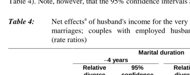
In the very shortest and the very longest marriages, the net effect of husband’s income was somewhat less clear. To see whether this was attributable to the comparatively low proportions of employed husbands in the shortest and the longest marriages, the same models were fitted to data including only the couples with employed husbands. As for marriages that had lasted for less than 5 years, the restriction to couples with employed husbands changed the result very little, and, as for the longest marriages, the restriction made the effect somewhat more consistently negative (see Table 4). Note, however, that the 95% confidence intervals are wide.
Table 4: Net effectsa of husband's income for the very shortest and the very longest
marriages; couples with employed husbands; relative divorce risks (rate ratios)
Marital duration
−4 years 30−39 years
Relative 95% Relative 95%
divorce confidence divorce confidence
risk interval risk interval
Husband’s income
1 (lowest) 1 1
2 0.98 (0.83−1.16) 0.80 (0.56−1.12)
3 0.93 (0.78−1.10) 0.84 (0.60−1.19)
4 0.99 (0.80−1.21) 0.82 (0.57−1.18)
5 (highest) 0.93 (0.71−1.22) 0.63 (0.43−0.95)
a
Net effect = the control variables as well as all other indicators of socioeconomic position are controlled for.
The sub-sample of couples with employed husbands includes ca. 160 thousand marriage-years of duration 0−4 years and ca. 255 thousand marriage-years of duration 30−39 years.
The gross effect models for housing density indicate that divorce risk increased with increasing housing density, but only among couples in their first or second decade in marriage. However, the differentials in divorce risk by housing density are explained by preceding socioeconomic factors, and the net effects of housing density show no direct effect of housing density on the risk of divorce in any of the duration segments.
7. Discussion
Using register-based data on Finnish women and men in their first marriages intact at the end of 1990 followed up for divorce between 1991 and 1993, this study explored the possibility that the effect of the socioeconomic position of spouses on the risk of divorce varies in marriages of various marital durations (up to the 40th anniversary of the wedding). Many socioeconomic factors, including spouses’ unemployment, wife’s income and employment, home-ownership, and the fact that the spouses were farmers were found to have similar effects on the risk of divorce in marriages of various durations. In contrast, the previously reported consistent differences in divorce risk between educational groups on one hand and between white-collar employee and manual worker groups on the other (Finnäs 2000, Jalovaara 2001) were found to be specific to marriages of relatively short duration. The findings are generally in line with those from the United States indicating that (wife’s) education is a more important predictor of marital disruption at early marital durations (Morgan and Rindfuss 1985, South 2001, South and Spitze 1986), whereas the effects of such factors as spouses’ employment, income, and material assets remain similar over marital careers (Booth et al. 1986, South and Spitze 1986, White and Booth 1991).
Prior research has reported that in Finland, the wife being a homemaker decreases the risk of divorce as compared to the wife being employed, but at the same time, both wife’s and husband’s unemployment increases the risk of divorce as compared to the spouses being employed (Jalovaara 2001, in press). The present study shows that the effects of spouses’ employment and unemployment are similar in marriages of various durations.
marriages that had lasted for less than 5 years, there were only 20 divorces to wives and 29 divorces to husbands who were pensioners.
The results indicate that overall, wife’s high income increases the risk of divorce irrespective of the duration of marriage. Husband’s high income was found to decrease the risk of divorce especially in marriages of medium durations. Particularly in the very shortest marriages, the net effect of husband’s income was weak and inconsistent, and this was not attributable to the comparatively low proportions of employed husbands at this marital duration. It is possible that income is a comparably poor indicator of a young husband’s personal characteristics and efforts, even if the husband is employed.
As compared to home-owners, the fact that the couple lived in a rented dwelling increased the risk of divorce irrespective of the duration of marriage. The lack of interaction with the duration of marriage is an unexpected finding, in that at longer marital durations, where home-ownership is highly prevalent, renters could be expected to be more strongly selected than in shorter marital durations in terms of factors predictive of divorce (such as a lowered expectation for the continuity of the marriage).
At the same time as the other socioeconomic factors exerted similar effects on the risk of divorce in almost all marital duration segments, wife’s and husband’s education and occupational class showed different patterns in shorter and longer marriages. Among marriages of short duration, the risk of divorce was strongly and negatively associated with the wife’s and husband’s level of formal education, whereas among marriages of comparatively long duration, divorce risk was highest for spouses having attained a secondary level education, even when such factors as spouses’ economic activity and income were considered. Further, the high divorce risk for manual workers as compared to white-collar employees was specific to marriages of shortest durations.
There are several potential explanations for these interactions. Firstly, the low divorce risk for spouses with high education and occupational position may be partly specific to the recent (birth and marriage) cohorts. During the increase in divorce in the early 20th century, divorce became an option not just for the wealthiest people, but for members of all social strata (Phillips 1991). However, even in 1946−47 in Finland, the divorce rate was much higher among men in professional occupations than among urban workers and lower white-collar employees (Allardt 1952, pp. 165−166). To the extent that the turn of the socio-structural divorce risk gradient from positive to negative is recent and it occurs at least partly over cohorts, it is one potential explanation for the failure to find negative educational and occupational divorce risk gradients for the longest marriages intact at the end of 1990.
marriage. Further, within a given birth cohort, spouses in marriages of short duration tend to be more highly educated, because the highly educated tend to marry at a later age. Therefore, it could be argued that the significance of having reached a certain educational level varies between spouses at various marital durations (see Hoem 19971). Among spouses in the longest marriages, those having no education beyond the basic level are the majority, whereas among spouses in the shortest marriages, they are much fewer and perhaps more strongly selected in terms of factors predictive of high marital instability.
However, the differences in divorce risk between white-collar employees and manual workers also declined with duration, although the differences between marital duration segments in distributions into these occupational classes were relatively modest. This suggests that explanations based on differential distributions may not be important.
Thirdly, the interactions between marital duration and education on one hand and between marital duration and occupational class on the other may also reflect genuine change across the phases of marital lives. Perhaps supporting this possibility, research from the United States that has followed successive cohorts of marriages as they are initiated reports that the negative impact of wife’s education on the risk of marital disruption disappears or turns positive with increasing marital duration (South 2001). Note that in longer marriages, the risk of divorce was highest for both husbands and wives with a secondary level education, and controlling for economic activity and income had little effect on the pattern. This finding lends little support to the hypothesis that in long marriages, highly educated women were likely to divorce because they have better chances of finding employment and having a high income.
The fourth and final potential explanation for the interactions is selective attrition, whereby differentials in divorce risk by a given permanent divorce-promoting characteristic decline or even reverse with the duration of marriage because marriages susceptible to that characteristics are selected out of the total pool of marriages at a higher rate than other marriages (see South and Spitze 1986, FN 6, Vaupel and Yashin 1985/1993). Given high rates of divorce during the first decades of marriage and the very strong effects of education and occupational class in marriages of short durations, selective attrition may be an important explanation for the differential divorce risk gradients for education and occupational class in shorter and longer marriages.
women among whom economic difficulties and the lack of material assets are commonplace and often temporary, as well as among men and women who have been together for decades and who are thought to be tied together by many kinds of tangible and intangible bonds that make a divorce costly. The pervasive nature of the effects of these factors highlights their importance as antecedents of divorce.
However, when measured in terms of wife’s and husband’s level of formal education and occupational class, an inverse association between the socioeconomic position of spouses and the risk of divorce was found only in the marriages of relatively short duration. These findings suggest that empirical research and the exchange-based theories concerning antecedents of divorce may need specification according to marital duration. The finding for occupational class suggests that the presence of differential educational distributions in the various birth cohorts is not a very likely explanation for the differential effects of education in shorter and longer marriages. It is likely that the interactions are partly related to developmental changes in marriages over the individual and marital life courses, and partly to differences between cohorts. A marked disadvantage of the present analysis was that it was based on a left-truncated study population and therefore, the effects of marital duration were confounded with the effects of cohort membership. A data set covering cohorts of marriages from the time they are initiated would allow patterns related to duration and cohort to be disentangled, and this in turn would greatly facilitate the interpretation of the interactions between temporal and socioeconomic determinants of divorce. Finally, the results of this study suggested that selective attrition may be an important factor in explaining the interactions between the duration of marriage and the socioeconomic factors. The cohort approach would also allow the importance of selective attrition to be estimated.
Acknowledgements
Notes
References
Aldous, J. (1990). “Family development and the life course: Two perspectives on family change”. Journal of Marriage and the Family, 52, 571−583.
Allardt, E. (1952). Miljöbetingade differenser i skilsmässofrekvensen: Olika normsystems och andra sociala faktorers inverkan på skilsmässofrekvenserna i Finland 1891−1950 [Environmentally conditioned differences in divorce rates: The effects of various norm systems and other social factors on divorce rates in Finland 1891−1950]. Helsingfors, Finland: Finska Vetenskapssocieteten.
Becker, G. S., Landes, E. M., and Michael, R. T. (1977). “An economic analysis of marital instability”. Journal of Political Economy, 85: 1141−1187.
Bengtson, V. L. and Allen, K. R. (1993). The life course perspective applied to families over time. In P. G. Boss, W. J. Doherty, R. LaRossa, W. R. Schumm, and S. K. Steinmetz (Eds.), Sourcebook of family theories and methods: A contextual approach, pp. 469−499. New York: Plenum Press.
Booth, A., Johnson, D. R., White, L. K., and Edwards, J. N. (1986). “Divorce and marital instability over the life course”. Journal of Family Issues, 7, 421−442. Finnäs, F. (1995). “Entry into consensual unions and marriages among Finnish women
born between 1938 and 1967”. Population Studies, 49, 57−70.
Finnäs, F. (1996). “Separations among Finnish women born between 1938
−
1967”.Yearbook of Population Research in Finland, 33, 21−33.
Finnäs, F. (1997). “Social integration, heterogeneity, and divorce: The case of the Swedish-speaking population in Finland”. Acta Sociologica 40, 263−277. Finnäs, F. (2000). “Ekonomiska faktorer och äktenskaplig stabilitet i Finland”
[Economic factors and marital stability in Finland]. Ekonomiska Samfundets
Tidskrift 53, 121−131.
Francis, B., Green, M., and Payne C., eds. (1993). The GLIM System. Release 4 Manual. Oxford, England: Clarendon Press.
Goldstein, J. R. (1999). “The leveling of divorce in the United States”. Demography,
Haskey, J. C. (1993). Formation and dissolution of unions in the different countries of Europe. In Blum, A. and Rallu J.-L. (Eds.), European Population, Vol. 2: Demographic Dynamics (pp. 211−229). Paris, France: Éditions John Libbey Eurotext.
Hoem, J. M. (1997). “Educational gradients in divorce risks in Sweden in recent decades”. Population Studies 51, 19−27.
Jalovaara, M. (2001). “Socio-economic status and divorce in first marriages in Finland 1991−93”. Population Studies, 55, 119
−
133.Jalovaara M. (in press). “The joint effects of marriage partners’ socio-economic positions on divorce risk”. Accepted for publication, Demography.
Kravdal, Ø. (1994). Sociodemographic Studies of Fertility and Divorce in Norway with Emphasis on the Importance of Economic Factors. Social and Economic Studies 90. Oslo-Kongsvinger, Norway: Statistics Norway.
Levinger, G. (1976). “A social psychological perspective on marital dissolution”.
Journal of Social Issues, 32, 21−47.
Lindgren, J. and Ritamies, M. (1994). Parisuhteet ja perhe [Unions and the family]. In Koskinen S., Martelin T., Notola I-L., Notkola V. and Pitkänen K. (Eds.), Suomen väestö (pp. 107−149). Helsinki, Finland: Gaudeamus.
Lutz, W., Wils, A. B. and Nieminen M. (1991). “The demographic dimensions of divorce: The case of Finland”. Population Studies 45, 437−453.
Morgan, S. P. and Rindfuss, R. R. (1985). “Marital disruption: Structural and temporal dimensions”. American Journal of Sociology, 90, 1055−1077.
Pensola, T. (2000). The Classification of Social Class After 1975: Differentiating Skilled Manual From Unskilled Manual Workers. Retrieved May 20, 2002, from http://www.valt.helsinki.fi/sosio/pru/ses.htm
Phillips, R. (1991). Untying the Knot: A Short History of Divorce. Cambridge, England: Cambridge University Press.
Pitkänen, K. (1986). “Marital dissolution in Finland: Towards a long-term perspective”.
Yearbook of Population Research in Finland, 24, 60−71.
Ross, H. L. and Sawhill I. V. (1975). Time of Transition: The Growth of Families Headed by Women. Washington, D.C., WA: The Urban Institute.
South, S. J. and Spitze G. (1986). “Determinants of divorce over the marital life course”. American Sociological Review 51, 583−590.
Statistics Finland (1992a) Vital Statistics 1989. SVT Population 1992:3. Helsinki, Finland: Statistics Finland.
Statistics Finland (1992b). Väestölaskenta 1990 opas [Census 1990 guide]. Handbooks 26. Helsinki, Finland: Statistics Finland.
Statistics Finland (2001). Vital Statistics 2000. SVT Population 2001:13. Helsinki, Finland: Statistics Finland.
Thornton, A. and Rodgers W. L. (1987). “The influence of individual and historical time on marital dissolution”. Demography, 24, 1−22.
VanLaningham, J., Johnson, D. R. and Amato P. (2001). “Marital happiness, marital duration, and the U-shaped curve: Evidence from a five-wave panel study”.
Social Forces, 79, 1313−1283.
Vaupel, J. W. and Yashin, A. I. (1993). Heterogeneity’s ruses: Some surprising effects of selection on population dynamics. In Bogue D. J., Arriaga E. E., and Anderton D. L. (Eds.), Readings in Population Research Methodology, Volume 6, Chapter 21, pp. 70−79. New York: The United Nations Fund for Population Activities. (Reprinted from The American Statistician, 39, 176−185, 1985.)
White, L. K. (1990). “Determinants of divorce: A review of research in the eighties”.
Journal of Marriage and the Family, 52, 904−912.
White, L. K. and Booth A. (1991). “Divorce over the life course. The role of marital happiness”. Journal of Family Issues, 12, 5−21.