Patron: Her Majesty The Queen Rothamsted Research Harpenden, Herts, AL5 2JQ Telephone: +44 (0)1582 763133 Web: http://www.rothamsted.ac.uk/
Rothamsted Research is a Company Limited by Guarantee Registered Office: as above. Registered in England No. 2393175. Registered Charity No. 802038. VAT No. 197 4201 51. Founded in 1843 by John Bennet Lawes.
Rothamsted Repository Download
A - Papers appearing in refereed journals
Leslie, P. H. and Gower, J. C. 1960. The properties of a stochastic model
for the predator-prey type of interaction between two species. Biometrika.
47 (3-4), pp. 219-234.
The publisher's version can be accessed at:
•
https://dx.doi.org/10.1093/biomet/47.3-4.219
The output can be accessed at:
https://repository.rothamsted.ac.uk/item/8w1w4
.
© Please contact [email protected] for copyright queries.
With 2 text-figures Printed in Oreat Britain
The properties of a stochastic model for the predator-prey type
of interaction between two species
B Y P. H. LESLIE AND J. C. GOWER
Bureau of Animal Population, Department of Zoological Field Studies, Oxford, and the Statistical Department, Rothamsted Experimental Station
1. INTRODUCTION
The two main types of interaction between any pair of biological species, which are of most interest to the ecologist, are either when they are competing together for some common source of food supply, or when one of the species preys upon the other. The properties of a stochastic model for a system of two competing species have been illustrated by a set of artificial realizations in an earlier paper (Leslie & Gower, 1958). We now consider some of the properties of a model for the interaction between a predatory species and its prey, more particularly in regard to the behaviour of such systems in the region of the stationary state, and the chances of random extinction for one or other of the two species. The interaction is imagined to take place in some limited environment where there is an ample supply of food for the prey, and in the first place it is assumed that all the members of the prey popula-tion are exposed to the risk of capture or attack by the predator. Later, this last condipopula-tion is relaxed, and it is supposed that because of some heterogeneity in the environment, only a fraction of the prey population is exposed to risk, and some of the consequences of this partial interaction are illustrated in the last section. The basic model has already been described (Leslie, 1948, 1958), but it will be useful if the formulae are summarized here.
If <Sr1 is a species of prey and St a predator, then working in discrete-time intervals and
given that the respective populations consist of N^t) and N2(t) individuals at time t, the
deterministic model for the interaction is taken to be,
where a1( y9j and a, are parameters > 0, and l o g ^ = r1 = 6j — dx, logeA2 = r2 = b% — dt are
the intrinsic birth- and death-rates of the two species. For the stationary state, 2^ -Lv
N3 = L2, we have,
0,(^-1) |
1
A(A
8-l)+o
1a,'L (1-2)
J
I t has been shown (Leslie, 1948, § 6) that this discrete-time model is closely related to the continuous-time model, (writing the operator D = djdt),
(a1,ai,cl>0), (1-3)
Biom. 47
220 P . H. LESLIE ASD J . C. GOWER
for which the stationary state is L, =
(1-4)
Putting Nx = Lx(\ + ttj) and Na = La(l + 1^), then we have from (1-3) for small 1^ and «j,
The equation in D is Z>a + (r, + Oji^) -D + ra(<h£i + c1Lt) = 0,
or from (1-4) Z^-Hrj + a ^ D + rir, = 0. (1-6)
The roots of (1*6), therefore, will be either both negative, or complex with the real part negative, so that the stationary state is stable, and an approach to this state will be made by a series of damped oscillations if
( i )2 < 4^7-,.
The properties of this model differ somewhat from those of the classical Lotka-Volterra equations for this type of interaction, viz.
1 = (el-y1Nt)N1 \
This deterministic system and the stochastic model based upon it have been discussed recently by Bartlett (1957 a). Here there is no damping towards the equilibrium point Lx = ej/y2, Lt = ejylt and the deterministic path of small cycles around this point is given
by the ellipse „ , . .
J r e%u\ + eyu\ = constant,
where Nt = Lx(l +«1),i^2 = Lt(\ + u^). Consequently, as Bartlett points out, in the stochastic
model the effect of random drift, in the absence of any damping factor, must result sooner or later, either in the extinction of the predator, or in the extinction first of the prey, followed in due course by that of the predator from starvation. In the stochastic formulation of this model (1-7), the stationary state is therefore in a sense unstable. But the presence of a damping term in the model defined by (1-3) would lead to a greater degree of stability, and in the corresponding stochastic model the system might therefore be expected to fluctuate in the region of the equilibrium state, although there might be still a chance of random extinction of one or other species, depending on the degree of variability in numbers in this region. To investigate this point, the stochastic discrete-time model corresponding to (1*1) was programmed for the Elliot-N.R.D.C. computer in the Statistical Department of Rothamsted Experimental Station, and some of the results obtained are given in the following sections.
2. STOCHASTIC MODEL
In a stochastic formulation of this model, a wide variety of possible birth-rate and death-rate functions for the two species could be adopted (cf. Leslie, 1958, §4). But, clearly, one of the most obvious choices to make is the case when the birth-rate (b) of each species remains constant, and any increase in the numbers of the predator affects the death-rate (d^t)) of the prey over the interval t to t + 1, and vice versa. If, therefore, in (1-1) we define the parameters representing the intrinsic birth- and death-rates of the two species,
Au = e*.-'v (a = 1,2; 6, ><*.,),
and put q^t) = 1+ a
we have in the constant birth-rate type of discrete-time stochastic model (Leslie, 1958, § 5),
E{Na(t+ 1) | #,(*). #2(0} = («-^a(0 = Aa(t)#a(0 (a = !. 2),
var{Na(t + 1)| Nx(t), Nt(t)} = & - l) (Aa(«) - 1) JS{^a(t + 1)} (21)
Here it is assumed that the difference between the constant birth-rate and the variable death-rate of each species at time t,
rjf) = log. [Aa/?.(0] = K-da{t) (a = 1,2)
remains constant over the interval t to t + 1, and that given N^t) and N2{t), then i^(t +1) and
Nt(t +1) are distributed normally and independently with these means and variances, all
negative values of Na(t + 1) being attributed to Na(t +1) = 0.
The programmes for this model were similar to those described by Leslie & Gower (1958) for a system of two competing species and little need be said of them here. In particular the same method of random number generation was used and the population parameters could easily be varied. Since the results consisted largely of long trajectories of the population numbers of the two species at succeeding instants of time, an additional programme was written to construct distributions of these population numbers direct from the output tapes.
3. THEORETICAL VABIANCES AND COVABIANCE OF THE SYSTEM
The theoretical variances and covariance of the population numbers, when such a Bystem is fluctuating in the region of the stationary state, may be estimated, to a first approxima-tion, in the following way. The equations (2-1) may be written in the form
(a = 1 , 2 ) (3-1)
in which the first term is the deterministic part of the process defined by (1-1); and the
Za(t +1) are independent normal variables with zero means, and variances, <r2(Za) ~ 2baLa.
when the birth-rate of each species remains constant, and the system is in the region of the stationary state (LltL%) defined by (1-2). By applying the usual iJ-technique (cf. Leslie &
Gower, 1958, §5), we have as a first approximation from (31), the set of equations for determining var (N^t)) — o\, var(i^(f)) = (T\ and cov ( ^ (
w
w
14-1
222 P . H . L E S L I E AND J . C. G O W E E
the partial differential coefficients being evaluated for Nt = Llt Nt = L%. ThuB, from (1-1)
and (1-2), we have
f X^
Jl 1
A
-A,
I t is also useful to have the equations for determining the variances and covariance for the analogous continuous-time model. From (1*5), writing Cj = kalt we have the linear
stochastic system for small v^ and Uj,
~ j (3-3)
in which the independent variables <5£ and 8<j> have zero means, and variances (2b1/L1) 8t
and (2bJLs) St, respectively, when the birth-rate of each species is assumed to remain
con-stant and the system is in the region of the state (L1( L2). From u^ + 8uv u^ + Su^, we finally
obtain, by squaring and taking the cross-product, the equations for the variances and covariance (<rf, ar\, tr]8) of v^ and u^,
bt
(3-4)
Yrt)crlt = ri(j\ — kaxLia\.
Since Nt = Lt(l +%), Nt = Ls(\ +«j), we then have
var (N-y) = L\ var (%), var (Nz) = LI var (u^), cov (Nlt Na) = LxLt cov (i^, u^),
which can be contrasted with the variances and covariance for the discrete-time model given by (3-2). The relationships between the parameters of the two types of model are
Ta = l o gsA0 (o = 1,2), Oj = c'i*']/(A1— 1) a n d k = Pil&i't
while the constant birth-rates 6X and b2, and the stationary values, Lt and L3, are naturally
the same for each model. In regard to the differences between the two models, it is perhaps worth noting that the variances estimated by means of (3-4) are always less than those obtained by the solution of (3-2), so that the use of the discrete-time model leads to an enhanced degree of variation when a particular system is fluctuating in the neighbourhood of the equilibrium level (cf. Bartlett, Gower & Leslie, 1960). By reducing the unit of time adopted in the discrete-time model, however, it is always possible to make the variances of the two types of model more in agreement.
223
4. FLUCTUATIONS IN THE NEIGHBOURHOOD OF THE STATIONABY STATE
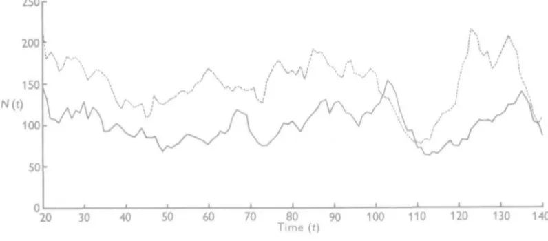
The behaviour of this type of system in the region of the stable stationary state may be illustrated by the results obtained from a realization which was computed for 1000 steps, taking as the numerical values of the parameters in (21)
Ax= 1-2574, b1 = 0-2577, A2 = 11892, 6, = 0-2521,
a, = 0-0005148, fil = 0-0018018 and Oj = 0-2838,
which from (1-2) give a stationary state of Lx = 150, Lt = 100. Starting with the initial
values of iV^(0) = 500 for the prey, and iV2(0) = 20 for the predator, these processes rapidly
approached their eauilibrium levels, in the recrion of which thev then continued to oscillate
250
200
150
N(t)
100
50
M A
20 30 40 50 60 70 80 90
Time (t)
100 110 120 130 1-40
Fig. 1. Fluctuations of a predator-prey system in the region of the stable stationary state. , the number of prey (equilibrium level Lr = 150); , the number of predators (equilibrium level Lt = 100).
in an irregular fashion. As an example, the changes in numbers are illustrated in Fig. 1 for the period of time from t = 20 to t = 140. I t will be seen that there is no regularity in the oscillations, and that at times there is a tendency for quite a pronounced excursion to be made away from the region of the stationary state, for example, in Fig. 1 the course of events from about t = 100 tot = 120, when a large fall in the numbers of the prey is followed shortly afterwards by a similar type of fall in numbers of the predator. The general picture is somewhat different from that of a system of two competing species with a stable stationary state (Leslie & Gower, 1958), where any drift away from the equilibrium level seems to take place in opposite directions owing to the negative correlation which exists between the two species in that type of system. In the case of the predator-prey type of interaction, the correlation is positive in sign.
Theoretically, it might be expected that the stationary distribution of such a two-species system would be approximately bi-variate normal in form, with variances and covariance given by (3-2), (Bartlett, Gower & Leslie, 1960). The bivariate distribution of N^t) and Nt(t)
is given in Appendix Table 1 for the last 800 steps in this realization. The observed means werei^x = 149-74and^s = 97-09, compared with the deterministic stable state of Lx = 150,
Lt = 100; while the observed variances and covariance (computed by the machine from the
224 P . H . L E S L I E AND J . C. G O W E B
individual observations and not from the grouped data), together with the values expected theoretically both for the discrete-time model, and for its continuous-time equivalent, were:
Expected
, *• » Observed Continuous-time Discrete-time Discrete-time
model model model
var(A'1) 432 546 636-6
var(Ag 170 228 214-0
cov {NltNt) +37-2 +56-6 +63-6
Considering that the expected values are based on the theory of small fluctuations and so cannot be exactly correct, the agreement in the case of the model actually used seems very satisfactory.
For samples as large as 800, taking g± ~ m^m\ and g% ~ [(mjml) — 3], we have (applying
Sheppard's corrections in computing the moments) for the marginal distribution of Nt in
Appendix Table 1,
gx ~ + 0-322±0087, gt 0-035±0-173,
and for that of Na, gx ~ +0-121 ±0-087, gz ~ -0-201 ±0-173.
The skewness coefficient for the second species is not much different from zero, while that for the first species is 3-7 times the standard error given, suggesting a degree of positive skewness in the marginal distribution of Nv These standard errors, however, are the
classical values, viz. c r ^ ) = ^/(6/n), ignoring the serial correlation between the successive values of both N^t) and N2(t). They are therefore underestimates of the correct values
(Bartlett et al. 1960). IH any case the degree of skewness is not very marked, and broadly speaking, we can regard the distribution given in Table 1 as being approximately bivariate normal in form.
5. T H E CHANCES OF RANDOM EXTINCTION
In the numerical system used as an illustration in the previous section, the chance of one or other of the species becoming extinot appears to be negligible, at least in terms of any ordinary time scale, once their numbers are in the region of their equilibrium levels. For instance, to take the predatory species which has the smaller numbers as an example; the order of magnitude of the mean passage time to extinction is likely to be inversely propor-tional to the probability of the zero state, or in terms of a normal distribution, using the observed mean and variance for this species, of the order of 1-4 x 10¹¹ units of time. I t
might be expected, therefore, that this system would continue to oscillate around the equilibrium level in an irregular fashion for a comparatively lengthy period. But, in other systems, this may not be so, and the chances of extinction may then become appreciable.
This point is relevant to the results obtained by Gause (1934) in his experiments with the two Protozoa, Didinium nasutum and Parameeium caudatum. The latter species is devoured by the former, and the amount of food required by Didinium is very great. His first experi-ments were carried out in a relatively small microcosm (the upper asymptote in numbers of the Paramecia, when living alone, being of the order of 100 individuals), and the introduction of small numbers of Didinium at varying intervals of time after the prey was followed by an intense multiplication of the predator, which devoured all the prey and afterwards themselves perished. There was also a considerable degree of variability in numbers between replicates of the same age (Gause, 1934, Chapter VI and Appendix, Table 6).
Suppose, then, we have a relatively small environment in which a species of prey is established, and which is then invaded by a small group of predators. For simplicity it will be assumed in the model that the intrinsic rates of increase and the birth-rates of both species are the same, and that in (2-1) we put
Ax = Ag = 1-25, b1 = bl = 0-25, Oj = 0-001.
These values of Ax and ax lead to a logistic upper-asymptote in numbers of the prey, if it
were living alone, of 250 individuals. When it is assumed that the birth-rates of both species remain constant, the remaining parameters, /?j and a,, in (1 • 1) and (2-1), define the magnitude of the effect which the numbers of each species have on the death-rate of the other. fi1 might
be termed t h e ' relative voracity' of the predator in regard to the prey, since for a given value of Ns, the greater the value of this parameter, the more the death-rate of the prey is affected
during a unit of time; and Oj represents the sensitivity of the predator to the relative density in numbers of the two species, i.e. for a given value of the ratio Nt/Nlt the greater the value
of Og, the more the death-rate of the predator is affected. Consider three systems in which /?x and <Zj are varied slightly, which together with the values pi the other parameters given
above lead to the following stationary states:
System A
0015 0025 0050
a, 0-375 0-500 0-260
22-7 18-6 4-9
£ | 15-2
9-3 4-9 (iii)
Some realizations were computed for each of these three systems, taking in each case = 200, Nt(0) = 15 as the initial conditions, i.e. it was assumed that the prey was well
established in this imaginary environment, when it was invaded by a small group of predators. The results were as follows.
System (i)
The computations were carried on for 399 steps, at the end of which time neither species was eliminated, though at one point the predator was very close to extinction, having been reduced to only one individual surviving on two successive occasions. Neglecting the first ten steps, during which time an approach was being made to the region of the stationary state, the observed means for the remaining 389 observations were fft = 25-33 and N% = 12-96;
while the observed variances and covariance compared with the theoretical expectations derived from (3-3) were
Expected Observed var (.?/,) 101 137-3 var(2tf,) 37-7 33-35
cov (NvNt) +19-7 +22-02
This very good agreement between the theoretical and observed variances was of interest, since in this type of discrete-time stochastic model, the assumption made in applying (2-1) that the Na(t+ 1) (o = 1,2), for given Na(t) are distributed normally, might be expected to
break down in the region of small numbers. The observed distributions of Nt and Nt are given
in Appendix Table 2, from which it can be seen that these departed appreciably from the normal, there being a pronounced positive skewness in each case. However, with no knowledge of the form of distribution which might be expected in such systems when numbers are small, it is difficult to know what reliance can be placed on this observed bivariate distribution.
226 P. H. LESLIE AND J. C. GOWER
System (ii)
The predator became extinct in each of the five realizations which were computed for this system. In one case the prey also vanished at the same time as the predator, and in another its numbers were reduced to only one individual. In this region of a stochastic logistic process, the probability of random extinction should be roughly of the same order of magnitude as that of a simple birth and death process with parameters corresponding to the intrinsic rate of increase of the particular species, viz. log A = b — d; so that if only one individual is left surviving, the probability that the prey population would in turn become extinct, is appreciable in this numerical example, being P(0) ~ djb = 011. In other words, the disappearance of the predator before the prey may not necessarily mean that the latter species will be able to persist.
System (iii)
Out of 19 realizations with the initial numbers NX(Q) = 200, Nt(0) = 15, the prey was
eliminated by the predator in 9 cases, which would result inevitably in the disappearance also of the predator. In the remaining 10, the predator became extinct before the prey; but
90
80
70
60
50
40
30
20
10,
5 10 15 20 25 30 35
Fig. 2. Representative trajectories for System (iii), for which the deterministic stable state is
LY = Lt ~ 5. The initial conditions were for the prey, N^O) = 200, and for the predator,
Nt(0) = 1 5 , but in order to save space, a few of the initial steps in each realization are omitted
from the figure.
in five of these cases the prey at this time was reduced to such low numhers, for example, either one or two individuals, that its ability to persist became problematical. There appeared to be little difference between the times taken for either predator or prey to become extinct, the combined mean passage time to extinction being I = 20-3 ± 2-99 units of time. The (Nlt N%) trajectories differed somewhat, depending on the length of time the interaction
persisted, but a pair of replicates are illustrated in Fig. 2, for which the passage time to zero was of the same order as the mean value. In broad outline the pattern is very similar to the trajectories observed by Gause (1934) in his experiments, not only with Didinium
and Paramecium, but also with other species of Protozoa, for example, Paramecium
bur8aria and Bursaria truncateUa (Gause, 1935).
The results with these three numerical systems suggest that, in a limited environment,
in which there is no immigration from outside, the persistence of both species in a
predator-prey interaction depends very greatly on the relations between the various parameters
for the two species, and that the chances of random extinction are very sensitive to relatively
small changes in these parameters. If the magnitudes of the intrinsic rates of increase of
the two species, the relative 'voracity' of the predator, and so forth, are not happily
adjusted in between themselves, it appears doubtful whether in a very simplified type of
system both species will be able to persist for very long, and the probability of random
extinction then becomes a dominant feature of the interaction.
6. WHEN ONLY A FRACTION OF THE PBEY POPULATION IS EXPOSED TO RISK
In developing the type of model we have used so far, one tacit assumption has been made,
namely, that in some way or other the entire prey population is exposed to the risk of
capture by the predator. The background environment in which the interaction takes
place is assumed to be in a sense' homogeneous', and the predator and prey populations freely
intermingle. Suppose, however, that this is not so, and that because of some' heterogeneity'
of the environment, only a fraction of the prey population is exposed to risk during any one
unit of time. One way in which this might occur would be if the configuration of some type
of vegetation formed a 'cover' for the prey, which protected it from the predator. Thus,
Gause (1934) has pointed out the importance of a refuge in enabling the prey to survive in
his experiments with various species of Protozoa, although the predator might still become
extinct. But, apart from 'cover' in its literal sense, a variety of different situations can be
imagined as regards the environment, or the habits of the two species, which would result
in the interaction being confined to only a fraction of the total prey population.
Suppose, for simplicity, that a fraction k (0 < k < 1) of the prey population is exposed
to risk of capture by the predator, and that this fraction remains constant for a particular
system. Then, in a more generalized model in the place of (1-1) and (21), the deterministic
part of the process may be written,
When k = 1, this system reduces to (1-1), and when k = 0, i.e. when none of the prey
population are exposed to risk, the predator cannot survive, and the system becomes a
simple logistic model for the prey population when living alone.
For the stationary state (L
lyL
t) of (6-1), we have for the predatory species
while that of the prey is given by the positive root of the equation,
n ( i t ) A , 1 t i . l ^ i 1 . ^ ( 6"2 )
1 + + \ L 0
U D ¥ l (
where B = a, +
a,
228 P. H. LESLIE AND J. C. GOWEB
The theoretical variances and covariance of the stochastic model for this type of system in the region of the stationary state may be obtained from (3-3), in a similar way to those of the original model, allowing for the alterations in the functions fx and/2.
I t is of interest to consider the effect of allowing the value of the constant k to vary in a system with a given set of the remaining parameters in (6-1), more particularly in regard to the chances of random extinction. As an illustration, take the System (iii) of the previous section, for which , , o n
Ax = Aj, = 1-25, <xx = 0-001, /^ = 0-050,
bx = b2 = 0-25, ctg = 0-250.
In this case it is known from the realizations already computed that the interaction cannot persist for very long, when k = 1. Suppose, now, that k is allowed to vary, and that a particular system with constant k is in the region of the stationary state (Lx, Lt) given by
(6-2). If, as an approximation, we assume that Nx(t) and N%(t) are both distributed normally
about means given by this state, then the mean passage time to zero for each species should be, very roughly, of the order of magnitude
&Jf>)~Jfrr)<r
aeW*'i (« = 1 , 2 ) ,
where the variance a\ is obtained from (3-3). The following are the stationary states (Lv L%)
and the estimated values of 0a(O) for a system with the basic parameters given above, over
a range of values of k (0 < k < 1).
Order of magnitude of the mean
k
0
0 0 5 0 1 0 0 1 5 0-20 0-25 0-35 0-50 0 0 5 0-80
1 0 0
Stationary state
i ,
250-0 230-1 1940 155-7 1250 90-7 50-4 23-3 12-8
8 1
4-9
0
11-5 19-4 23-4 2 5 0 22-7 17-6 11-6
8-3 6-5 4-9
passage time to
9,(0)
5-8 x 10" 9-8x10" 6-0x10" 7-4 x 10" 1-2x10" 1-5x10" 2-4x10* 3-3xlO«
76
37 20
zero in units
0,(0) —
6-2 x 10* 1-3 xlO4 4-8x10* 6-5 xlO4 1-7 xlO4 1-5 x 10» 1-6 x 10«
58 34 21
It will be seen that, as might be expected, the stationary numbers of the prey (Lx)
steadily increase as a smaller fraction of the population is exposed to risk; while those of the predator (L%) steadily increase with decreasing k up to a maximum which, in this
par-ticular example, is reached in the region of k = 0-20. The estimates of ©a(0), which must
not be taken too literally, change very rapidly as k decreases. Taking the figures for the predator, which is the species having the smaller numbers, it appears that the approximate maximum mean passage time to extinction is reached at k ~ 0-20, when it is about 3000 times greater than in the case of the original system with k = 1. These estimates of 0a(O)
suggest that in this particular system both species would persist for a comparatively long time when some 10—35 % of the prey population were exposed to risk, in contrast with the relatively rapid extinction of one or other species as this fraction approaches unity.
It was of interest, experimentally, to see how far some of these figures could be confirmed in practice. Taking k = 1 in the model, 100 realizations were computed, starting each time
with the initial numbers iV^O) = N3(0) = 5, i.e. the nearest integers to the deterministic
stationary state. In 51 of the replicates the predator disappeared before the prey, the mean passage time to the zero state being I = 19-61 + 2-27 units. In the remaining 49 the prey became extinct before the predator, with I = 19-25 ± 2-55. The distributions of the in-dividual times to extinction were very skew, the longest time recorded being in the
t = 76-79 class.* But these mean figures are in excellent agreement with those given in the
table above. It is also of interest to note that these mean times may be very little affected by the initial numbers adopted in this particular system, as was illustrated in the previous section (System iii), when with N^O) = 200, N2(0) = 15, the combined mean passage time
to extinction for 19 replicates was t ~ 20 units.
When k = 0-8 in this system, the 'normal' approximation suggests that the mean passage time to zero should be of the order of 35 steps for both species. In 50 realizations using this value of k, and taking as the initial state -^(0) = 8, ^ ( 0 ) = 7, the predator became extinct in 38 cases, with 1= 43-55 ±6-36; while in the remaining 12, the prey disappeared in I = 50-17 + 11-48 steps. Both of these means are somewhat greater than the expected figure, but the distributions of the individual times were even more skew than in the preceding examples when k = 1, the interaction on one occasion persisting for 172-175 steps before the predator became extinct. In general, however, these computed mean times to extinction for the two values of k are in reasonably good agreement, at least as regards orders of magnitude, with those derived from the normal approximation.
A further realization was computed for the case of k = 0-20, for which, according to the above table, the chance of the predator being able to persist is at a maximum, and starting with the initial numbers of N^O) = 125, Na(0) = 25, the calculations were carried on for
999 steps. During this time there appeared to be no definite approach to the zero state, although on one occasion the numbers in the predator population fell to only six individuals. The observed means for the 999 observations were N± = 120-75, Nt = 22-37, compared
with the deterministic stationary state of Lx = 125, Lt = 25; and the variances and
co-variance were var(i^) = 345-2, var(i^) = 37-66 and cov (NvNa) = +8-24. These observed
variances are in very good agreement with the theoretical approximations derived from (3-3), namely <x\ ~ 296, <rf ~ 37-4 and cr12 ~ +7-53. The grouped frequency distribution of Nx and N2 is given in Appendix Table 3, and from the marginal distributions we have for
the prey species (NJ ^ _0.1 6 8 ± 0.0 7 7 > ^ . _0-089± 0-155,
and for the predatory species (Nt)
gx ~ + 0-131 ±0-077, ga 0133±0155,
where the standard errors attached to the estimates are again the classical values, repre-senting lower limits to the correct values. The magnitude of the skewness coefficiente suggests that the distribution can be regarded as approximately bivariate normal in form. But, the main point of these results is to confirm that in this system, both species should co-exist for comparatively lengthy periods of time when, owing to some ' heterogeneity' of the environment, the fraction of the prey population exposed to risk is of the order
• In carrying out these computations, the machine was instructed to stop whenever the number of one or other species reached zero, and to record the number of steps taken for this point to be reached. Although the means and variances were computed from the individual figures, the frequency distribu-tions of the times to extinction were finally printed in groups of four units, so that it is impossible to give the exact highest and lowest figure observed.
230 P. H. LESLIE AND J. C. GOWER
of 20 %. Naturally, this optimum fraction, which reduces the chance of random extinction of the predator to a minimum, will vary from system to system and may indeed be insufficient to prevent the disappearance of one or other species.
The ' heterogeneity' of the environment is not, however, the only factor which would tend to increase the probability of both species co-existing. The relative dispersion and movements of the two species over an area may also be important. This has been illustrated very elegantly by some experiments by Huffaker (1958) with the mite Eotetranychus
aexmactdaius as the prey, and the predator mite, Typhlodromus occidentalis, in which a
number of oranges, arranged in trays in a two-dimensional manifold, were used as the medium on which the prey species could develop. In all his simple universes, the inter-action did not persist for very long, either the predator or prey disappearing as in Gause's experiments with various species of Protozoa, to which we have referred. But, when in Huffaker's experiments partial barriers were included in his universe, the co-existence of the predator and prey was maintained for three successive oscillations of the system. This more complex environment, in which the partial barriers restricted the movements of the species from orange to orange arranged in a two-dimensional grid, made it less likely that the predator would be in contact with the prey at all positions simultaneously. In a stoch-astic model for this type of system it would be necessary to incorporate a spatial grid, with restricted or partially restricted movements of the individuals from cell to cell, as in the model designed by Bartlett (19576) for studying theoretically the development of a measles epidemio in a community. In terms of the simplified models used here, the nearest approach one could make to such a system would be to consider that the fraction k of the prey popula-tion exposed to risk was not a constant, but a variable; although at first sight it is not easy to see what form of functional dependence of k on the relative numbers of the two species should be adopted in the model. Generally speaking, however, it seems likely from the results for constant k given in this section, that even in the case of variable k, provided that this variability is not too extreme, the likelihood of both species being able to co-exist would be greatly increased.
REFERENCES
BARTXBTT, M. S. (1957a). On theoretical models for competitive and predatory biological systems. Biometrika, 44, 27-42.
BARTLBTT, M. S. (19576). Measles periodicity and community size. J.R. Statist. Soc., A, 120, 48-70. BARTLETT, M. S., GOWER, J. C. & LESIXE, P. H. (1960). A comparison of theoretical and empirical
results for some stochastic population models. Biometrika, 47, 1-11.
GAUSE, G. F. (1934). The Struggle Jor Existence. Baltimore: Williams and Wilkins.
GAUSE, G. F. (1935). Verifications experimentales de la theorie mathematique de la lutte pour la vie. Actualitis Sri. no. 277, 1-61. Paris: Hermann.
HUTTAKEK, C. B. (1958). Experimental studies on predation: dispersion factors and predator-prey oscillations. Hilgardia, 27, 343-83.
LWST.TK, P. H. (1948). Some further notes on the use of matrices in population mathematics. Biometrika. 35, 213-45.
T.KHT.nc, P. H. (1958). A stochastic model for studying the properties of certain biological systems by numerical methods. Biometrika, 45, 16-31.
T.gBT.ra, P. H. & GOWER, J. C. (1958). The properties of a stochastic model for two competing specie*. Biometrika, 45, 316-30.
APPENDIX I
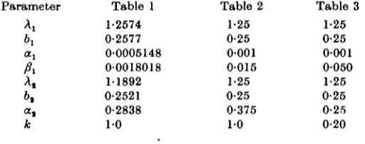
For convenience, the bivariate distributions of Nt and Nt in the region of the stationary state for the three systems, to which reference has been made in the text, are given all together in this appendix. These grouped frequency distributions were tabulated by hand from the typed lists of results for each series, the marginal totals being checked by the distributions of each species (grouped in pairs of integers. 0-, 2-, 4-, ft-, etc.) recorded by the machine. It should be noted, however, in this connexion that all the variances and covariances given in the text were calculated on the machine from the individual results in each series, and not from the grouped data. They are therefore, in a sense, exact. The following were the values of the parameters used in computing the processes.
imeter
1
ai
A
A,a* k
Table 1 1-2674 0-2677 0-0005148 00018018 11892 0-2621 0-2838
1 0
Table 2 1-25 0-25 0-001 0-015 1-25 0-25 0-375
1 0
Table 3 1-25 0-25 0-001 0-050 1-25 0-25 0-25 0-20
to
w
Table 1
80- 90- 100- 110- 120- 130- 140- 160- 160- 170- 180- 190- 200- 210- 220- Total
56- 60- 64- 68- 72- 76- 80- 84- 88- 92- 96- 100- 104- 108- 112-116— 120- 124- 128- 132- 136- 140-1 1 2 1 1 2 1 1 1 3 2 3 1 2 2 2 1 3 4 2 9 8 6 8 7 2 2 4 3 1 1 2 1 2 7 8 3 14 7 9 5 5 3 2 1 2 1 t 3 6 5 9 11 10 12 20 13 5 8 14 2 5 2 2 1 2 4 7 10 8 8 10 20 12 14 9 5 8 3 1 1 1 . 2 3 1 5 4 8 7 13 13 15 6 13 10 5 2 3 1 1 2 2 4 5 9 10 14 7 13 8 4 6 5 4 5 1 3 3 2 1 1 6 6 6 4 11 6 13 2 8 3 4 1 1 1 1 3 5 5 5 6 7 4 3 1 1 2 2 2 2 3 3 1 2 2 2 1 2 4 2 3 2 1 2 3 1 2 1 2 1 1 1 , 1 0 17 15 22 34 61 61 72 84 97 79 64 56 57 29 17 18 5 7 3 1 M M
°
QTotal 1 9 22 61 72 128 123 112 105 74 42 22 15 9 5 800
2V, 0- 12- 10- 20-
24-Table 2
28- 32- 36- 40- 44- 48- 52- 56- 60- 64- 68- Total
0- 2- 4- 6- 8- 10- 12- 14- 16- 18- 20- 22- 24- 26- 28- 30-
32-Total 0
2 5 8 8 16 14 9 4
10 17 44 69
1 5 3 6 15 7 8 4 4 4 2 3 1 1
64 1 6 6 11 3 5 5 4 1
1 1 1
1
45 2 2 6 12 4 3 7 3 2 1 1 3
46 25 17 23
2 12 21 29 39 69 55 46 40 26 17 12 7 7 6 0 1
389
Is3
Table 3
60- 60- 72- 78- 84- 90- 96- 102- 108- 114- 120- 126- 132- 138- 144- 150- 156- 162- 168- 174- Total
6- 8- 10- 12- 14- 10- 18- 20- 22- 24- 26- 28- 30- 32- 34- 30- 38- 40-Total # 1 1 1 3 1 3 1 1 1 1 8 1 1 2 2 . 1 7 2 1 1 1 5 2 1 1 1 1 3 4 1 14 3 . 4 7 4 5 4 4 2 2 2 2 1 40 1 2 3 5 8 9 8 9 12 9 7 2 4 1 80 1 3 4 5 7 11 15 16 3 11 5 5 1 1 2 90 3 1 6 10 10 20 14 16 10 6 1, 6 4 1 10S 4 9 5 9 11 19 17 13 16 9 4 2 2 2 1 123 1 3 3 7 7 8 9 13 19 10 6 2 9 7 2 2 1 109 1 4 6 7 8 9 11 14 15 11 9 4 3 1 1 1 105 1 3 3 9 2 11 11 17 11 15 11 1 4 2 1 1 103 1 2 2 8 6 11 9 10 14 6 3 7 2 2 2 91 1 1 2 4 2 4 13 14 7 7 5 4 1 2 07 2 4 1 5 3 3 1 7 2 2fi 1 1 2 2 1 1 8 2 1 2 1 (1 1 1 2 9 27 39 64 73 97 128 141 124 110 09 37 35 23 12 7 2 999 co O O