Desert 23-1 (2018) 97-106
Effectiveness of spectral data reduction in detection of
salt-affected soils in a small study area
M. Rahmati
a*, N. Hamzehpour
aa
Department of Soil Science, Faculty of Agriculture, University of Maragheh, Maragheh, East Azarbayjan, Iran
Received: 16 Desember 2017; Received in revised form: 19 March 2018; Accepted: 22 April 2018
Abstract
Data reduction is used to aggregate or amalgamate the large data sets into smaller and manageable information pieces in order to fast and accurate classification of different attributes. However, excessive spatial or spectral data reduction may result in losing or masking important radiometric information. Therefore, we conducted this research to evaluate the effectiveness of the different spectral data reduction algorithms including Principle Component Analysis (PCA) and Minimum Noise Fraction (MNF) transformation, Pixel Purity Index (PPI), and n Dimensional Visualizer (n-DV) algorithms on accuracy of the supervised classification of the salt-affected soils applying ETM+ data beside 188 ground control points. Results revealed that data reduction caused around 20 to 30 % decreases in classification results compared to none reduced data. It seems that applying spectral data reduction algorithm in small study areas is not only supportive, but also has negative effects on classification results. Therefore, it may better to not to use the algorithms in small areas.
Keywords: Modeling; Regression modeling; Salt-affected soils; Salinity; Satellite images
1. Introduction
Hyperspectral and multispectral imaging technology have been widely used to detect salt-affected soils. For example, Metternicht (2001) predicted spatiotemporal soil salinity using fuzzy logic, remote sensing and GIS. Malins and Metternicht (2006) also evaluated spatial variations of soil salinity in rain fed lands in the west of Australia. Odeh and Onus (2008) predicted soil salinity using GIS, remote sensing with salinity, normalized salinity and brightness indices. Soil salinity mapping in Mexico (Fernandez-Buces et al., 2006); soil salinity variations trend in soil profile in South Africa (De Clercq et al., 2009); analysis of the dynamics of saline soils in China (Yu et al., 2010); and regional-scale soil salinity assessment using Landsat ETM+ canopy reflectance (Scudiero et al., 2014; Scudiero et al., 2015; Rahmati et al., 2014; Rahmati and
Corresponding author. Tel.: +98 912 5419200
Fax: +98 41 37276060
E-mail address: [email protected]
Hamzehpour, 2016) are other examples for the benefits of remotely sensed data in soil salinity monitoring and prediction.
Pal et al., 2011), and n-Dimensional Visualizer (n-DV) (Ahmad, 2012) algorithms. Several researchers (Eriksson and Viberg ,2000; Vanlanduit et al., 2004) have applied different data reduction algorithms in order to increase the accuracy of the classifications. For example, Zhang et al. (2015) applied spatial and spectral data reduction algorithms quantifying their effects on classification accuracies. Their results revealed that spatial and spectral data reductions improved classification accuracies, decreased computer constrains, and reduced analytical concerns of classifications of the large and high-dimensional datasets.
Although, it may reduce the levels of stochastic noise and levels of autocorrelation among adjacent spectral channels, excessive spatial and spectral data reductions may result in losing or masking important radiometric information (Zhang et al., 2015). Therefore, regarding both fast data processing and robust and accurate data classification, it seems that researcher needs to check the consequences of different data reduction algorithms on the accuracy of the classification models in different situations. Specifically, the necessity for application of the spectral data reduction in small study area is on doubt. Therefore, the current research was aimed to assess the effectiveness of the different data reduction algorithms including PCA and MNF transformation, PPI, and n-DV algorithms on
accuracy of the supervised classification of the salt affected soils in a small study area.
2. Materials and Methods
2.1. Study area, Soil Sampling, and ETM+ data acquisition
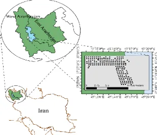
The current research was carried out in an area with longitudes of 45֯ 09' 00"E to 45֯ 17' 00"E and latitudes of 37֯ 24' 00"N and 37֯ 30' 00"N located in East Azerbaijan province, northwest of Iran (Fig. 1). In this regard, 188 soil samples were taken from the study area on a grid of 500 m. Soil samples were taken from 0-25 cm depths and then they were analyzed for their EC in 1:2.5 soil to water extractions. ETM+ data of the study area for sampling dates also were acquired free of charge from
http://earthexplorer.usgs.gov/. Since bands 6
and 8 of ETM+ data are thermal bands and differ from others, only bands 1 to 5 beside band 7 were applied in this investigation. Prior to image analysis, we georeferenced all images using zone 38 and datum WGS84. The images were also corrected for their gaps resulted from malfunctioning of Landsat scan line corrector using Landsat gapfill application of ENVI. Atmospheric correction also was applied on satellite images using dark object subtraction method.
2.2. Remote Sensing of Soil Salinity
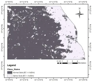
Supervised classification is applied to map salt-affected soils. In this regard, we applied 188 soil samples as Ground Control Points (GCP’s) and maximum likelihood as classification method to map salt-affected soils. In order to classifiy salt-affected soils using maximum liklihood algorithm, we applied 80% of GCP’s to train the algorithm. In this case, first we catogrized all sampled points into two groups of normal soils having EC < 4 dS/m and saline soils having EC ≥ 4 dS/m. Therefore, 149 out of 188 sampled points categorized as normal soils showing EC < 4 dS/m and 39 points categorized as saline soils showing EC ≥ 4 dS/m. Applying
80 % for each group, we randomly devided GCP’s into two groups of train and test data. Therefore, 119 points of normal soils beside 31 points of saline soils were randomly selected to train the classification algorithm.
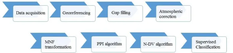
We repeated classification for three times applying three different data. First, we applied original bands of ETM+ data (bands 1 to 5 and 7) to map salt-affected soils (Fig. 2). Second, prior to classification, we applied PCA to select uncorrelated factors to map salt-affected soils (Fig. 3). Third, the MNF transformation, PPI, and n-DV algorithms were applied to construct uncorrelated factors to map salt-affected soils (Fig. 4).
Fig. 2. Applied processes to classify saline and non-saline soils using original bands of ETM+ data
Fig. 3. Applied processes to classify saline and non-saline soils using uncorrelated bands of PC analysis
Fig. 4. Applied processes to classify saline and non-saline soils using uncorrelated bands of MNF transformation, PPI, and n-DV algorithms
2.3. Principle Component Analysis
The PC analysis was applied to extract uncorrelated factors of the original bands of ETM+ data. An orthogonal transformation was used in PCA, as a statistical procedure, to convert a set of observations into a set of values of linearly uncorrelated variables called principal components (Peason, 1901) and ENVI software was used to construct the main factors.
2.4. MNF transformation, PPI, and n-DV algorithms
Spectral Identification System (ORASIS), Iterative Error Analysis (IEA), Convex Cone Analysis (CCA),and Automated Morphological Endmember Extraction (AMEE) have been developed to extract pure pixels automatically via remote sensing data (Bouaziz et al. 2011). Boardman et al. (1995) reported that PPI index is one of the successful procedures to define pure pixels. We applied automated spectral hourglass (ASH) application in ENVI software to construct uncorrelated factors using MNF transformation, PPI, and n-DV algorithms.
2.5. Model Performance Assessment
We applied confusion matrix to evaluate classification results. Confusion matrix is pixel by pixel comparison of ground trust data with mapped pixels. In order to construct confusion matrix, we divided GCP’s into two groups of training and test data. In this regard, we applied 80% of all data (150 out of 188) to train the classification algorithm and the rest (20 %, 38 out of 188) to check the results. Then, following criteria were applied to assess the classification results:
2.5.1. Overall accuracy
Overall accuracy (OA) averages classification accuracy dividing correctly classified pixels by all applied ground trust data:
1
C ii i
OA
X N (1)where, Xii is the number of correctly classified
pixels in class i (values of diagonal arrays of confusion matrix), C is the number of classes, and N is the number of ground trust data. OA criterion usually overestimates the classification accuracy.
2.5.2. Kapa coefficient
Kapa coefficient (K) is calculated using following formula: . . 1 1 2 . . 1 C C
ii i i
i i
C i i i
N X X X
K
N X X
(2)where, Xii is values of diagonal arrays of
confusion matrix, Xi. and X.i are summations for
arrays in row and column i, respectively, and C
and N are the numbers of classes and ground trust data, respectively. Contrary to OA, Kapa coefficient calculates classification accuracy into a totally random classification. In the other word, it eliminates the effect of chance in classification and calculates the correspondence with ground trust data. K coefficient near to 1 implies the best classification; K coefficient near to zero implies totally random classification, and K coefficient lower than zero implies weak classification. It is important to mention that K coefficient usually underestimates the accuracy of the classification.
2.5.3. Producer’s accuracy
Producer’s accuracy (PA) illustrates classification accuracy of a single class which is calculated using following equation:
1 ii j C ij i
X
UA
X
(3)where, Xii is values of diagonal array of
confusion matrix for row and column i and Xij is
each array in row i and class j.
3. Results
3.1. Visual image analysis of whole Urmia Lake watershed
Salt-affected soils are easily detectable by applying visual analysis of satellite data and selecting proper false color composite (FCC). Elnaggar and Noller (2009) applying ETM+ data reported that salt-affected soils show high reflectance in visual (bands 1, 2 and 3) and NIR (band 4) bands and low reflectance in SWIR (bands 5 and 7).
Table 1. Created false color composites (FCC) beside their I and OIF factors
Number& False color composite I factor OIF factor
1 145 0.231 1862.81
2 157 0.100 1806.03
3 135 0.156 1795.15
4 147 0.275 1767.64
5 345 0.178 1750.51
6 125 0.248 1718.12
7 137 0.158 1687.87
8 235 0.189 1687.49
9 357 0.079 1673.10
10 245 0.183 1671.47
11 347 0.209 1665.49
12 134 0.142 1651.78
13 127 0.251 1608.61
14 257 0.084 1605.15
15 237 0.190 1586.94
16 247 0.217 1584.75
17 234 0.153 1569.74
18 124 0.204 1564.78
19 457 0.041 1515.00
20 123 0.096 1369.03
&: Composites are filtered in descending order based on OIF factor
Figure 5 displays constructed FCC using bands 1, 4 and 5. Figure 5 beside field assessments revealed that areas with deep water of Lake Urmia are in brown red, shallow water are in light red, playa is in yellow, highly saline
soils around the Lake Urmia are in gray, and the remains which are non-saline soils are in combination of blue and green. Cloud contaminations in Figure 5 are shown in white.
Fig. 5. Lake Urmia watershed- images mosaic of ETM+ data in Autumn 2009
3.2. Classification of salt-affected soils using original bands of ETM+ data
As first step, we applied original bands of ETM+ data in supervised classification algorithm to map salt-affected soils though study area (Fig. 6). Constructing confussion
for normal and saline soils, respectively, it revealed that 76.67% of normal soil and 100 %
of saline soils were classifed correctly based on the independent test data.
Fig. 6. Classification map of saline and non-saline soils using supervised classification and original bands of ETM+ data without any data reduction algorithm
Table 1. Evaluation results of classified map using supervised classification method and all original bands of ETM+ data
Class/Parameter Normal soils Saline soils All
OA (%) - - 81.58
K - - 0.580
PA (%) 76.67 100 -
3.3. Classification of salt-affected soils using main factors of PCA
First, we applied PCA to construct uncorrelated factors. Since we applied 6 original bands of ETM+ data as input data for PCA, six
main factors also were consturcted which we chose two first factors (PC1 and PC2) for further processes. In this regard, we applied eigenvalue curve of constructed factors (Fig. 7) to select the main factors for further processes.
Regarding Figure 7, since PC1 and PC2 demonstrate 94% of variations together, we selected PC1 and PC2 to apply as input data in classification algorithm. Then, we applied supervised classification algorithm and maximum likelihood method beside PC1 and PC2 data to map salt-affected soils (Fig. 8).
Table 3 reports the evaluation results for classified map.
Classified map showing OA of 56.63% and K coefficient of 0.18 revealed very low accuracy for applied data. Although, obtained PA of 87.50 % reveals reasonably high accuracy for saline soils, PA of 43.33 % reports very low accuracy for non-saline ones.
Fig. 8. Classification map of saline and non-saline soils using supervised classification and main factors extracted from PCA
Table 3. Evaluation results of classified map using supervised classification method and selected main factors of PC analysis
Class/Parameter Normal soils Saline soils All
OA (%) - - 52.63
K - - 0.18
PA (%) 43.33 87.50 -
3.4. Classification of salt-affected soils using
main factors extracted from MNF
transformation, PPI, and n-DV algorithms
A series of data reduction algorithms including MNF transformation, PPI, and n-DV algorithms were applied prior to any classification to construct uncorelated factors. Constructing uncorrelated factors using MNF transformation, PPI, and n-DV algorithms, we used 199716 pixels to extract pure pixels (Fig. 9-A). In order to set the parameters of the ASH tool for pure pixels’ extraction, the number of the MNF bands, number of PPI iterations, threshold value of PPI, and maximum number of the applied PPI pixels were set to be 6, 5000, 2.500, and 10000, respectively. The Mixture
Tuned Matched Filtering (MTMF) and Spectral Angle Mapper (SAM) methods were used as mapping methods. We applied eigenvalue curve of MNF bands (Fig. 9-B) to choose final MNF bands for further analysis. According to Figure 9-B, MNF bands 1 to 3 showing 94 percent variances were selected for further process which finally resulted in 4 nD-classes. Figure 9-C and 9-D depict MNF values for selected bands and PPI curve, respectively.
A
D
C
B
applied data. Although, the classified map showed relatively high accuracy obtaining PA of 87.50 and 67.56 % for saline and non-saline
soils, respectively, the weakness of the classification is clear in K coefficient (K=0.29).
Fig. 9. Pure pixels extracted by PPI index within study area (A), eigenvalue curve of the constructed MNF bands (B), MNF values for selected bands (C), and the number of the selected pixels per each iteration (D)
Table 2. Evaluation results of classified map using supervised classification method and constructed semi-image from MNF transformation, PPI, and n-DV algorithms
Class/Parameter Normal soils Saline soils All
OA (%) - - 63.16
K - - 0.29
PA (%) 67.56 87.50 -
4. Disscussion
The results showed that supervised classification using original bands of ETM+ data had reasonably high accuracy for predicting salt-affected soils showing OA of 81.75 %. Supervised classification algorithm has been applied for several times by different researchers. For example, Abbas et al. (2013) applied the algorithm to classify soil salinity reporting an OA of 90 %. Wu et al. (2008) also applied supervised classification to map soil salinity and the results also revealed higher accuracy for this algorithm reporting OA of 90 to 98 %.
The results revealed that supervised classification algorithm applying all original bands of ETM+ data with OA of 81.75 % showed higher accuracy than applying main factors extracted from PC analysis with OA of 56.63 % and MNF transformation, PPI, and n-DV algorithms with OA of 63.16 %. It sounds that data reduction algorithms may be more useful for application in vast areas. There may be no need for data reduction algorithms through our study area consisting small area. Zhang et al. (2015) have discussed that, although, data reduction may decrease the risk for overfitting of the classifying model due to the Hughes phenomenon (Guo et al., 2008; Lu
et al., 2011) and the risk of overfitting or
violation of the principle of parsimony (Hawkins, 2004), excessive spatial or spectral data reduction may mask or loose important radiometric information. On the other hand, data reduction algorithms may be more appropriate for hyperspectral imaging data which are typically acquired at high spatial (serval pixels per square millimeter) and spectral resolutions (spectral channels with wavelength ranges less than 10 nm) (Ariana and Lu 2010; Gowen et al. 2011; Zhang et al. 2015) However, several researchers also have applied supervised classification beside data reduction algorithms to map salt-affected soils. For example, Shirazi
et al. (2013) applied supervised classification
algorithm beside PCA data reduction algorithm to map soil salinity. They also applied DEM map as auxiliary data to improve classification results. Their results revealed that applying PCA algorithm beside DEM map increased the accuracy of the classified maps reporting an OA
of 97 to 99 %. However, it seems DEM data application cannot increase the accuracy of our classification results since the variation for elevation of our study area is not considerable.
5. Conclussion
This paper evaluates the effectiveness of the different data reduction algorithms on classification results of the salt-affected soils using spectral data of ETM+ images. The results allowed drawing of the following conclusions: 1) the supervised classification method is satisfactory to map salt-affected soils, 2) applying PCA as spectral data reduction algorithm decreased the accuracy of the classification results through study area as a small region, and 3) applying MNF transformation, PPI, and n-DV algorithms as spectral data reduction algorithm also decreased the accuracy of the classification results through study area as a small region.
Acknowledgments
This work was supported by the office of Vice Chancellor for Research, University of Maragheh under Grant 94/d/3471.
Rrferences
Abbas, A., S. Khan, N. Hussain, M. A. Hanjra, S. Akbar, 2013. Characterizing soil salinity in irrigated agriculture using a remote sensing approach. Physics & Chemistry of the Earth, Parts A/B/C, 55; 43-52. Ahmad, F., 2012. Pixel Purity Index Algorithm and n- Dimensional Visualization for ETM+ Image Analysis: A Case of District Vehari. Global Journal of Human Social Science Arts & Humanities, 12; 76- 82.
Ariana, D. P., R. Lu, 2010. Evaluation of internal defect and surface color of whole pickles using hyperspectral imaging. Journal of Food Engineering, 96; 583-590.
Boardman, J. W., F. A. Kruse, R. O. Green, 1995. Mapping target signatures via partial unmixing of AVIRIS data. Pasadena, California, USA.
Bouaziz, M., J. Matschullat, R. Gloaguen, 2011. Improved remote sensing detection of soil salinity from a semi-arid climate in Northeast Brazil. Comptes Rendus Geoscience, 343; 795-803.
Elnaggar, A. A., J. S. Noller, 2009. Application of remote-sensing data and decision-tree analysis to mapping salt-affected soils over large areas. Remote Sensing, 2; 151-165.
Eriksson, J., M. Viberg, 2000. Adaptive data reduction for signals observed in spatially colored noise. Signal Processing, 80; 1823-1831.
Fernandez-Buces, N., C. Siebe, S. Cram, J. Palacio, 2006. Mapping soil salinity using a combined spectral response index for bare soil and vegetation: A case study in the former lake Texcoco, Mexico. Journal of Arid Environments, 65; 644-667.
Fruchter, B., 1954. Introduction to factor analysis. Published by D. Van Nostrand Co.
González, C., J. Resano, D. Mozos, A. Plaza, D. Valencia, 2010. FPGA implementation of the pixel purity index algorithm for remotely sensed hyperspectral image analysis. EURASIP Journal on Advances in Signal Processing, 2010; 1.
Gowen, A., F. Marini, C. Esquerre, C. O’Donnell, G. Downey, J. Burger, 2011. Time series hyperspectral chemical imaging data: Challenges, solutions and applications. Analytica Chimica Acta, 705; 272-282. Green, A. A., M. Berman, P. Switzer, M. D. Craig, 1988. A transformation for ordering multispectral data in terms of image quality with implications for noise removal. IEEE Transactions on Geoscience & Remote Sensing, 26; 65-74.
Guo, B., S. R. Gunn, R. I. Damper, J. D. Nelson, 2008. Customizing kernel functions for SVM-based hyperspectral image classification. IEEE Transactions on Image Processing, 17; 622-629.
Hawkins, D. M., 2004. The problem of overfitting. Journal of Chemical Information & Computer Sciences, 44; 1-12.
Hotelling, H., 1933. Analysis of a complex of statistical variables into principal components. Journal of Educational Psychology, 24; 417.
Lavenier, D. D., J. P. Theiler, J. J. Szymanski, M. Gokhale, J. R. Frigo, 2000. FPGA implementation of the pixel purity index algorithm. Information Technologies 2000, International Society for Optics and Photonics.
Lu, H., H. Zheng, Y. Hu, H. Lou, X. Kong, 2011. Bruise detection on red bayberry (Myrica rubra Sieb. & Zucc.) using fractal analysis and support vector machine. Journal of Food Engineering, 104; 149-153. Malins, D., G. Metternicht, 2006. Assessing the spatial extent of dryland salinity through fuzzy modeling. Ecological Modelling, 193; 387-411.
Metternicht, G., 2001. Assessing temporal and spatial changes of salinity using fuzzy logic, remote sensing and GIS. Foundations of an expert system. Ecological Modelling, 144; 163-179.
Odeh, I. O., A. Onus, 2008. Spatial analysis of soil salinity and soil structural stability in a semiarid region of New South Wales, Australia. Environmental Management, 42; 265-278.
Pal, S., T. Majumdar, A. K. Bhattacharya, R. Bhattacharyya, 2011. Utilization of Landsat ETM+ data for mineral-occurrences mapping over Dalma and Dhanjori, Jharkhand, India: an Advanced Spectral Analysis approach. International Journal of Remote Sensing, 32; 4023-4040.
Peason, K., 1901. On lines and planes of closest fit to systems of point in space. Philosophical Magazine, 2; 559-572.
Rahmati, M., M. Mohammady Oskouei, M. R. Neyshabouri, A. Fakheri Fard, A. Ahmadi, J. Walker, 2014. ETM+ data applicability to remote sensing of soil salinity in Lighvan watershed, Northwest of Iran. Current Opinion in Agriculture, 3; 10-13.
Rahmati, M., N. Hamzehpour. 2016. Quantitative remote sensing of soil electrical conductivity using ETM+ and ground measured data. International Journal of Remote Sensing, 38; 123-140.
Scudiero, E., T. H. Skaggs, D. L. Corwin, 2014. Regional scale soil salinity evaluation using Landsat 7, western San Joaquin Valley, California, USA. Geoderma Regional, 2; 82-90.
Scudiero, E., T. H. Skaggs, D. L. Corwin, 2015. Regional-scale soil salinity assessment using Landsat ETM+ canopy reflectance. Remote Sensing of Environment, 169; 335-343.
Shirazi, M., G. R. Zehtabian, H. Matinfar, S. Alavipanah, 2013. Evaluation of LISS-III Sensor Data of IRS-P6 Satellite for Detection Saline Soils (Case Study: Najmabad Region). Desert, 17; 277- 289.
Vanlanduit, S., P. Guillaume, J. Schoukens, 2004. Robust data reduction of high spatial resolution optical vibration measurements. Journal of Sound & Vibration, 274; 369-384.
Wu, J., B. Vincent, J. Yang, S. Bouarfa, A. Vidal, 2008. Remote sensing monitoring of changes in soil salinity: a case study in Inner Mongolia, China. Sensors, 8; 7035-7049.
Yu, R., T. Liu, Y. Xu, C. Zhu, Q. Zhang, Z. Qu, X. Liu, C. Li, 2010. Analysis of salinization dynamics by remote sensing in Hetao Irrigation District of North China. Agricultural Water Management, 97; 1952- 1960.