Estimating and Forecasting Demand for Broad Money
in Iran through Cointegration Analysis and Stochastic
Simulation
Gholam Reza Eslami-Bidgoli∗ Saeed Bajalan∗∗ Mehdi Mirza Bayati∗∗∗
Abstract
his study estimates the demand for broad money in Iran through multivariate Cointegration analysis as proposed by Johansen and Juselius and tests the validity of the estimated model through forecasting money demand for several periods Using stochastic simulation technique. The study obtained one unique cointegrated long run relationship among the logarithmic forms of Broad Money, National Income, Exchange Rate, Price Index and Oil Prices. After identification of exogenous variables, system of equation was designed and estimated by OLS method. Model was solved by considering two scenarios: Baseline and Scenario1.In the Baseline the variables were considered endogenous and in the Scenario 1, Price Index and Oil Price were regarded as exogenous. This model was solved with stochastic simulation approach and give dynamic forecast of the variables. The results show that there is trivial difference between actual values and amount forecasted under Scenario1. On the other hand, forecasted amounts by Baseline scenario have relatively substantial deviations from the actual outcomes, though they do seem to follow the general trends in the data very well.
Keyword: Cointegration Analysis, Johansen Approach, Weak
Exogeneity, Stochastic Simulation.
∗ Associate Professor of University of Tehran, E-mail: [email protected].
∗∗ Master of Finance, Financial Analyst of Tejarat Bank.
1- Introduction
The demand for money function represents one of the most valuable aspects of the monetary process in a market economy. The demand for money reflects the degree of willingness to possess money by economic entities/agents (Mankiw, 1997: 476).
The appropriate money demand function indicates (1) whether there are alternative assets available in the economy to hold money; (2) how liquid the money and capital markets are; (3) whether the interest rates are controlled by the authorities or determined by market forces; (4) how fast financial innovation is taking place in the economy; and (5) whether a country can influence the exchange rates (Gurley and Shaw, 1960: 179-190).
The money demand function links money and other real economic variables and it plays an important role in the decision making process of central banks in dealing with monetary and exchange rate policies. It plays a major role in macroeconomic analysis, especially in selecting appropriate monetary policy actions.
The majority of the studies on money demand functions have been confined to industrial countries. However, studies carried out in developing countries have been increasing in recent years. This increase in studies has been attributed to the concern about the impact of moving towards flexible exchange rate regimes, globalization of capital markets, ongoing financial liberalization, financial innovations in domestic markets, and emergence of new financial assets and country specific events on money demand like political transformation and huge changes in oil prices which heavily affect country income and the cost of production.
The rest of this paper organized as follow:
Section 2 provides empirical literature about the issue. In section 3, the data and econometric model are described. The data characteristics and empirical results are presented in section 4. Finally, section 5 provides summary of findings and conclusions.
2- Literature Review
According to recent development in the econometrics of nonstationary data, Hoffman and Rasche applied econometric techniques (Johansen, 1988, 1991) had been designed to account for the nonstationarities that prevail in the variables that constitute money demand. They find a cointegrating relation among real M1 balances, short-term interest rates, and real personal income, using U.S. data at monthly intervals (Haffman & Rasche, 1991).
They further provided strong evidence for the stability of the long-run demand function for narrowly defined money (M1) in five industrial countries (U.S., Japan, Canada, U.K. and West Germany) using post-war quarterly data (Haffman&Rasche, 2003). and chose the economically meaningful results. The study found that all variables were significant and the scale variables have the expected positive signs while the interest rate/opportunity cost variables had negative signs. The variables that showed a rapid speed of adjustment to equilibrium were inflation, income and foreign interest rates. Using the Chow test, the demand for money equation was tested for structural stability and it proved to be stable. The major weakness of the study, as noted by the author, was the use of monthly data over a relatively short time period (ten years). Despite the fact that monthly data increased the number of observations with which to conduct statistical analysis, high frequency data is relatively noisy, hence, there can be a problem of extracting efficient signals from it (Adam, 1991: 401).
was -0.36 while for M2 was very low at -0.12 and both interest rate variable were statistically significant (Hafer and Jansen, 1991: 164). The analysis of the stability of both functions provided evidence that M2 is the preferable measure with which to consider the long run economic impacts of changes in monetary policy.
Sebastian Arango and M. Nadiri generalized traditional demand functions for money to take account of foreign monetary developments, such as changes in the exchange rates. The demand function for real cash balances deduced from this model was shown to depend upon domestic variables such as real income, the interest rate, as well as actual and anticipated foreign monetary development. The model was estimated using quarterly time series data for the period 1960 to 1975 from three major industrialized countries: Canada, the United Kingdom, and U.S (Arango&Nadiri, 1981: 69).
Baba et al. (1992) confirmed the results by Hafer and Jansen (1991)
study by finding a stable cointegrating money demand function for real M1 and variables: real GNP, one month Treasury bill rate, inflation rate, yield on M1 and moving standard deviation of holding periods on long term bonds. By using Johansen and Juselius (1990) approach and having all variables in logarithms to ensure that the model was equivalent under a range of transformations of dependent variables, they found that the treasury bill rate elasticity was -39%, own rate 12% and inflation -14%. The long run income elasticity was, 0.5 and therefore, consistent with the Baumol (1952) - Tobin
(1956) theory (Baba et al., 1992: 41).
McNown and Wallace concluded that the effective exchange rate is necessary for M2 demand cointegration in the United States, using quarterly data from 1973:2 to 1988:4 (McNown and Wallace, 1992: 107). Following them, Bahmani-Oskooee and Shabsigh (1996) gaive empirical evidence for this hypothesis with regard to the Japanese economy using quarterly data from 1973: l to 1990:4. The researchers concluded that the effective exchange rate is necessary for M2 demand cointegration based on the fact that there is no evidence for M2 cointegration without the effective exchange rate, but there is evidence for M2 cointegration when the effective exchange rate is added.
indicated that the effective exchange rate is necessary for Japanese M2 demand cointegration.
Ericsson (1998) found one cointegrating vector in the study of demand for money using M1, total final expenditure (TFE), three month authority interest rate, retail deposit interest rate and inflation as variables, based on the United Kingdom quarterly data from 1963:1 to 1989:2 and using parsimonious conditional equilibrium model with all variables in logarithms except interest rates (Ericsson, 1998: 307). The income elasticity was found to be unitary in the long run and coefficients of interest rates and inflation were sensibly signed. In the short run, elasticities of money with respect to prices and income were both close to zero.
Sriram (1999a) estimated the demand for money function in Malaysia, a small open economy, initially by applying a closed economy model framework and later an open economy model by allowing for possibilities of currency substitution. Based on the cointegration and weak exogeneity tests, the study found that the long run income elasticity is close to one and the opportunity cost variables (interest rates on alternative assets and inflation) were negatively related to money as expected. However own rate of money was positive (Sriram, 1999a: 19). These results are therefore, consistent with theory.
Besides papers listed above, several studies have been conducted in Iran on the issue of estimation of demand for money. Mostafavi and Yavari (2007) tried to estimate demand for money in Iran by using time series and Cointegration analysis for the period of 1988-2004. Their model involved GDP, inflation, rate of return of foreign exchange and automobiles. Conitegraion test has been applied via Auto Regressive Distributed Lag and Johansen procedure. Results revealed that GDP and inflation affect money demand in the long run and those factors plus the foreign exchange rate of return are significant in the short run.
for short run dynamic analysis showed that the speed of adjustment toward long run balance is slow.
Shahrestani and Sharifi (2008) used the same approach for estimating money demand in Iran. Cointegrated and stable long run relationship among M1, income, inflation and exchange rate exist in Iran economy according to their research. They found that income elasticity and exchange rate coefficients are positive while the inflation elasticity is negative. They concluded that, depreciation of domestic currency against foreign currency increases the demand for money and so people prefer to substitute physical assets for money. In addition their work showed that M1 demand function was stable between 1985 and 2006.
3- Data and Econometric Model
Demand for money function in this paper was estimated by using following variables: real demand of broad money (M2), National Income (GNP), nominal exchange rate (EXH), oil price (OIL), and Price levels which is represented by Consumer Price Index (CPI).
All data are obtained from the Central Bank of Islamic Republic of Iran. The sample period in this study is from 1979: 3 to 2006:2 and the forecast period covers period of 2006:3-2007:2 (the latest data available in database of Central Bank of Islamic Republic of Iran).
The natural logs of above variables are used in model in order to make interpretation of results straight forward. For example, while we can not easily interpret the CPI (t)-CPI (t-1), the deference of log of this variable means inflation.
The order of integration of each variable in the study is identified through Augment Dickey Fuller test (ADF). The details of the test are in the next part. It appears that the level of each series is nonstationary but the first difference of each series is stationary so the Johansen approach is appropriate to estimate the model. In the below this approach has been described briefly:
correct approach. However, when the relationship among variables is important, such a procedure is inadvisable. While this approach is statistically valid, it does have the problem that pure first difference models have no long-run solution. The finding that many macro time series may contain a unit root has spurred the development of the theory of non-stationary time series analysis. Engle and Granger (1987) pointed out that a linear combination of two or more non-stationary series may be stationary. If such a stationary linear combination exists, the non-stationary time series are said to be cointegrated. The stationary linear combination is called the cointegrating equation and may be interpreted as a long-run equilibrium relationship among the variables. There are several ways for testing for cointegration such as Granger, Granger 2 step method, Engle-Yoo 3-step method. Among these models Johansen technique based on VARs not just give method for testing cointegration but also for estimating cointegration systems.
Suppose that a set of g variables (
g
≥
2
) are under consideration thatare I(1) and which are thought may be cointegrated. A VAR with k lags
containing these variables could be set up:
t t k t k t
t
t y y y Ax u
y =
β
1 −1+β
2 −2+...+β
− + +In order to use the Johansen test, the VAR above needs to be turned into a Vector Error Correction Model (VECM) of the form:
t t k
t k t
t
t y y y y Ax u
y = +ΓΔ +Γ Δ + +Γ Δ + +
Δ
π
t-1 1 −2 2 −2 .... −( −1)In fact the Johansen test can be affected by the lag length and so it is useful to attempt to determine the optimal lag length. This can be achieved
by using information criteria such as AIC or HQIC.
π
could be interpretedas a long run coefficient matrix since in the equilibrium, all the Δyt−i will be
zero and setting the error term,ut, to their expected value of zero will leave
0 1=
−
t
y
π
,The test for cointegration among the
y
sis calculated by looking at therank of the
π
matrix via its eigenvalues. The eigenvalues, denotedλ
iareput in ascending order:
g
λ
λ
There are two test statistics for cointegration under the Johansen approach, which are formulated as follow:
∑
+ =− −
= g
r i
i
trace r T
1
) 1 ln( )
(
λ
λ
and
) 1 ln( )
1 ,
( 1
max r r+ =−T −
λ
r+λ
Where r is the number of cointegration vectors under the null
hypothesis and
λ
i is the estimated value for ith order eigenvalue from theπ
matrix.
λ
trace is a joint test where the null is that the number of cointegrationvectors is less than or equal to r while
λ
maxconduct separate tests on eacheigenvalue, and has as its null hypothesis that the number of cointegrating
vectors is r against an alternative of r+1.
π
can not be full rank (g) since this means to the original ytbeingstationary. If
π
has zero rank, then by analogy to the univariate case there isno long run relationship between the elements of yt−1. For 1≤
π
<g , thereare r cointegrating vectors.
π
is then defined as the product of two matricesα
andβ
′:β
α
π
=
′
The matrix
β
gives the cointegrating vectors, whileα
gives theamount of each cointegrating vector entering each equation of the VECM also known as the “adjustment parameters”. (Brooks, 2002)
After estimating long run relationship among M2, National Income, Exchange Rate, Price Levels and Oil prices, the authors have tried to build a model and solving it through Stochastic simulation in order to forecast M2 for the period of 2006:3-2007:2 and test the validity of the estimated model.
4- Empirical Results 4-1- Stationarity test
information criteria considered. The result supports the notion that each series is integrated of order one over the sample period. It is worth noting that because Lm2 series look like to be trended, both intercept and trend were included in ADF test equation.
Table1: Result of ADF test for stationarity
Variables ADF Test
Statistic
10% Critical Value
5% Critical Value
1% Critical Value
Test Result
Log Level of each series
L*(CPI) -0.419904 -2.581596 -2.889200 -3.493747 Fail to reject
L(GNP) 0.084722 -2.581313 -2.888669 -3.492523 Fail to reject
L(M2) -1.763915 -3.151673 -3.452358 -4.046072 Fail to reject
L(EXH) -1.857095 -2.581313 -2.888669 -3.492523 Fail to reject
L(OIL) -1.426292 -2.581176 -2.888411 -3.491928 Fail to reject
Log deference of each series
L(CPI) -3.614072 -2.581596 -2.889200 -3.493747 Reject
L(GNP) -4.478493 -2.581313 -2.888669 -3.492523 Reject
L(M2) -4.111325 -3.151673 -3.452358 -4.046072 Reject
L(EXH) -3.620038 -3.492523 -2.888669 -2.581313 Reject
L(OIL) -8.956192 -2.581041 -2.888157 -3.491345 Reject
H0: Null hypothesis: series has a unit root.
*L: letter shows the Logarithm
4-2- Cointegration test
As it stated in the above, ADF test reveals that all variables are nonstationary but they are integrated of order 1. Hence, the standard VAR(k) model equation can be transformed into a Vector Error Correction Model(VECM) to estimate long run relation between variables. In order to
determine the cointegrating rank r, trace test (
λ
trace) and the maximumeigenvalue test (
λ
max), proposed in Johansen (1991) are utilized. If seriesboth of them. As a rough guide if all series seems to have stochastic trend, just intercept term should be included in both inside and outside of cointegration relation. On the other hand, if some of series are trend stationary, intercept and trend term are included inside cointegration relation and just intercept outside of it. Since Lm2 series shows sign of deterministic trend, we use later case in order to test the presence of cointegration among variables. The result of test of existence of Cointegration Equation (CE) among variables was presented in table2.
Table2: Result of Cointegration Test
Hypothesized
No. of CE Eigenvalue Trace Statistic
5 Percent Critical Value
1 Percent Critical Value
None ** 0.375575 112.7969 87.31 96.58
At most 1 0.201596 62.87892 62.99 70.05
At most 2 0.159971 39.01403 42.44 48.45
At most 3 0.118046 20.53621 25.32 30.45
At most 4 0.065853 7.220924 12.25 16.26
*(**) denotes rejection of the hypothesis at the 5% (1%) level
Trace test indicates 1 cointegrating equation(s) at both 5% and 1% levels
Hypothesized
No. of CE Eigenvalue
Max-Eigen Statistic
5 Percent Critical Value
1 Percent Critical Value
None ** 0.375575 49.91797 37.52 42.36
At most 1 0.201596 23.86489 31.46 36.65
At most 2 0.159971 18.47782 25.54 30.34
At most 3 0.118046 13.31529 18.96 23.65
At most 4 0.065853 7.220924 12.25 16.26
*(**) denotes rejection of the hypothesis at the 5% (1%) level
Max-eigenvalue test indicates 1 cointegrating equation(s) at both 5% and 1% levels
Table3: Normalized Cointegration Coefficients and Adjustment Coefficients
Normalized cointegrating coefficients (std.error. in parentheses and t statistics in [ ] )
LM2 LGNP LCPI LOIL LEXH @TREND
1.000000 0.416183 -0.515204 0.573669 0.032343 -0.033729
(0.18879) (0.12531) (0.05277) (0.09903) (0.00402)
[ 2.20443] [-4.11143] [-10.8711] [ 0.32661] [-8.38277]
Adjustment coefficients D*
(LM2) D(LGNP) D(LCPI) D(LEXH) D(LOIL)
-0.132783 -0.209907 0.041959 -0.374903 0.248399
(0.03182) (0.07365) (0.03461) (0.11882) (0.23925)
[-4.17315] [-2.85009] [ 1.21236] [-3.15529] [ 1.03823]
* D sign shows the first difference.
The results have been shown in table 3 indicate that the long run income elasticity (0.416183) is far from unity which is proposed by the quantity theory of money. The lower than unity income elasticity suggests that money demand has been rising at a rate, lower than the changes in total transactions in the economy. The direction of effects of income on real money demand is well known and therefore needs no further discussion. However, it would be useful to comment briefly on the direction of the effect of the exchange rate on money demand. If people expect the domestic currency would be rebound they hold more domestic money and this increase the money demand but if they expect further depreciation of domestic money, they would want to reduce their domestic money holding. In this paper the second case seems to be true although the coefficient of this variable is not statistically significant.
The coefficient of LCPI was expected, a priori, to be either negative or
positive. It turned out to be negative and this means that when inflation increases, opportunity cost of holding money will be increased so people demand less money. Finally, the positive sign of LOIL reveals that with the increase in oil prices, the government increases its demand for money and therefore injects money into economy body of the country.
The coefficient of (-0.132783) shows that the speed of adjustment is approximately 13 percent, that is, when there is deviation from equilibrium, more than 13 percent is corrected in one quarter as the variable moves
towards restoring DLM2 equilibrium.Thus, there is strong pressure on the
stock of money to restore long run equilibrium whenever there is a disturbance. The high speed of adjustment may reflect the existence of banking facilities and high returns on financial assets which can allow economic agents to re-establish equilibrium levels of money holdings faster (Hayo, 2000: 588, Sriram, 1999a: 20).
4-3- Weak exogeneity test
Tests of weak exogeneity are carried out by placing a zero restriction
on the loading factor (matrix of error correction terms) in equation
π
=α
β
′,that is α = 0. The coefficients in the α matrix capture the speed of adjustment
of a particular variable to a deviation from the long run equilibrium. Therefore a zero restriction on any coefficient in this matrix will correspond to the null hypothesis that the particular variable does not adjust to restore the long run equilibrium and hence can be regarded as weakly exogenous or otherwise, the variable is endogenous.
Since cointegration tests confirmed one relationship, the weak
exogeneity tests are conducted under the assumption of(r)=1 (r is the
number of cointegrated relationship)
Table4: Test of Weak Exogeneity
Variable Likelihood Ratio Statistic Probability
LM2 14.52971 0.000138
LGNP 7.260909 0.007047
LCPI 1.359579 0.24361
LEXH 9.152122 0.002484
LOIL 1.101986 0.293831
4-4- Testing the Validity of Model
After identification of exogenous variables in the model, the forecasting power of the model in giving reasonable estimation of the future has been tested. In order to achieve to this purpose at first system of equations was built. Note that when the purpose is to estimate the unknown coefficients in the stochastic equations, OLS method could not simply be used since endogenous variables appears on the right-hand side of several of the equations as an independent variable but is endogenous to the system as a whole. Because of this, we would expect endogenous variables to be correlated with the residuals of the equations, which violate the assumptions of OLS estimation. To adjust for this, some form of instrumental variables or system estimation would be needed to use. In this paper the second approach was preferred. The results of estimation were showed that the model did not suffer from serial correlation.
By using the result of systems’ parameters estimation, we built our model. Model was solved with considering two scenarios: Baseline and Scenario1. In Baseline all the variables were considered as endogenous while in the Secnario1 LCPI and LOIL as were regarded as exogenous variables, which showed the symptoms of weak exogeneity in section 4.3.
0 1 2 3 4 5 6 7 8
80 82 84 8688 90 92 9496 98 00 0204 06 Actual
LCPI (Baseline Mean) LCPI (Scenario 1 Mean)
LCPI ± 2 S.E.
0 1 2 3 4 5 6 7 8 9
80 82 84 8688 90 92 9496 98 00 0204 06 Actual
LOIL (Baseline Mean) LOIL (Scenario 1 Mean)
LOIL ± 2 S.E.
10.0 10.4 10.8 11.2 11.6 12.0 12.4 12.8 13.2
80 82 84 86 88 90 92 94 96 98 00 02 04 06 Actual
LGNP (Baseline Mean) LGNP (Scenario 1 Mean)
LGNP ± 2 S.E.
-12 -11 -10 -9 -8 -7 -6 -5 -4
80 82 84 86 88 90 92 94 96 98 00 02 04 06 Actual
LEXH (Baseline Mean) LEXH (Scenario 1 Mean)
LEXH ± 2 S.E.
7 8 9 10 11 12 13 14 15 16 17
80 82 84 86 88 90 92 94 96 98 00 02 04 06 Actual
LM2 (Baseline Mean) LM2 (Scenario 1 Mean)
LM2 ± 2 S.E.
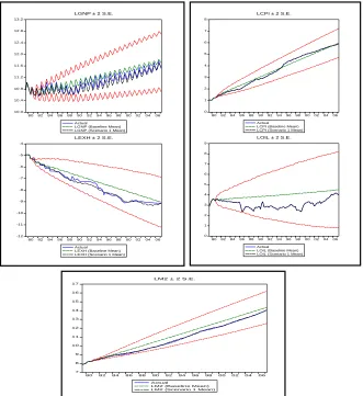
Because of our purpose, testing forecasting power of model, we also used dynamic forecast rather than static. Indeed, when we want to evaluate model in predicting many periods into the future, we must use our forecast from previous periods, not actual historical data, in order to assign values to the lagged endogenous terms in the model. The result of forecasting has been presented in Figure1.
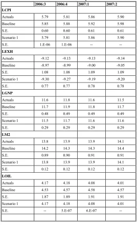
In addition, projections for the period of 2006:3 – 2007:2 provided in the table5. It is evident the projections under Scenario1 are outperformed Baseline both in forecasted amounts and standard deviations of them.
Table 5: the forecasted amounts for the period of 2006:3-2007:2
2006:3 2006:4 2007:1 2007:2 LCPI
Actuals 5.79 5.81 5.86 5.90
Baseline 5.85 5.88 5.92 5.98
S.E. 0.60 0.60 0.61 0.61
Scenario 1 5.79 5.81 5.86 5.90
S.E. 1.E-06 1.E-06 -- --
LEXH
Actuals -9.12 -9.13 -9.13 -9.14
Baseline -8.97 -8.99 -9.00 -9.05
S.E. 1.08 1.08 1.09 1.09
Scenario 1 -9.30 -9.27 -9.19 -9.20
S.E. 0.77 0.77 0.78 0.78
LGNP
Actuals 11.6 11.8 11.6 11.5
Baseline 11.7 11.9 11.8 11.7
S.E. 0.48 0.49 0.49 0.49
Scenario 1 11.5 11.7 11.6 11.6
S.E. 0.29 0.29 0.29 0.29
LM2
Actuals 13.8 13.9 13.9 14.1
Baseline 14.2 14.3 14.3 14.4
S.E. 0.89 0.90 0.91 0.91
Scenario 1 13.8 13.9 13.9 14.1
S.E. 0.12 0.12 0.12 0.12
LOIL
Actuals 4.17 4.18 4.08 4.01
Baseline 4.53 4.57 4.58 4.57
S.E. 1.87 1.89 1.91 1.91
Scenario 1 4.17 4.18 4.08 4.01
The results illustrate how our model would have performed if we had used it back in 1981:1 to make a forecast for variables over the next 26 years. In the scenario1, we implicitly assume that the amounts of exogenous variables are known at the time the forecasts were generated. On the other hand, in Baseline we suppose that the amount of all variables are unknown at the time of forecasts and determine all of them through solving model. The above figures show that scenario1 have outperformed in contrast with Baseline. Indeed there is trivial difference between actual values and amount estimated under Scenario1. According to above figures, in general, forecasts under Baseline scenario have relatively substantial deviations from the actual outcomes, although they do seem to follow the general trends in the data very well.
The error bounds in the resulting output graph show that we should be reluctant to place too much weight on the point forecasts of the model, since the bounds are quite wide.
5- Conclusion
This study aimed at describing the nature of money demand in Iran through considering its long run relationship with other major macroeconomic variables as proposed by literature. The empirical estimations found a number of interesting results.
Firstly, and most importantly, the results of this study confirmed that there exists a unique cointegrating relation among the demand for broad money (M2) and National Income (GNP), Price Levels (CPI), Foreign Exchange Rate and Oil Prices.
Secondly, the long run income elasticity has significant deviation from unity proposed by the quantity theory of money. In the long run Oil Prices have significant positive effect on M2 while Price Levels negatively affects this variable. Exchange rate has not significant impact on M2.
considered as endogenous although even under this assumption, model could forecast the general trend exactly.
References
1-ADAM, C., 1991. “Financial innovation and the demand for M3 in the
UK 1975-86”. Oxford Bulletin of Economics and Statistics. 53 (4): 401-424.
2-Arango, S., Nadiri, M. I., 1981. “Demand for money in open
economies”, Journal of Monetary Economics, 1981,7,69-83
3-BABA, Y., HENDRY, D. F. and STARR, M. R., 1992. “The demand
for M1 in the U.S.A., 1960-1988”. Review of Economic Studies. 59 (1):
25-61.
4-Bahamani-Oskooee, M., Shabsigh, G., 1996 “ The demand for money in
Japan: evidence from cointegration analysis”, Japan and the World
Economy, 8, 1-10
5-BROOKS, C., 2002. “Introductory Econometrics for Finance”.
Cambridge: Cambridge University Press.
6-Dikey, David A., and Sastry G. Pantula, 1987, “ Determining the Order
of Differencig in Autoregressive Processes” Journal of Business &
Economic Statistics, Vol. 5, No. 4 (October), 455-61
7-Engle, Robert F., and C.W.J Granger, 1987, “ Co-Integration and Error
Correction: Representation, Estimation and Testing” , Econometrica, Vol.
55, No. 2 (March), 251-276
8-Hoffman, D,L., Robert H. Rasche, 1991. “Long-run income and interest
elasticity of money demand in the United States”, The Review of Economics
and Statistics, 7
9-Hoffman, D, L., Robert H. Rasche, 2003. “The stability of long-run
money demand in five industrial countries”, Journal of Banking and
Finance, 27,575-592
10-ERICSSON, N. R., 1998. “ Empirical modeling of money demand”.
Empirical Economics. 23: 295-315.
11-GURLEY, C. J. and SHAW, E. S., 1960. “ Money in a theory of
finance 3rd ed” ED. Washington DC: Connecticut Printers.
12-HAFER, R. W. and JANSEN, D. W., 1991. “The demand for money
in the United States: evidence from cointegration tests”. Journal of Money,
Credit, and Banking. 23 (2): 155-168.
13-HAYO, B., 2000. “The demand for money in Austria”. Empirical
14-Johansen, S., 1988. “Statistical analysis of cointegration vectors”.
Journal of Economic Dynamics and Control. 12: 231-254.
15-Johansen, S., and Juselius, K., 1990. “Maximum likelihood estimation
and inference on Cointegration - with applications to the demand for
money”. Oxford Bulletin of Economics and Statistics. 52 (2): 169- 210.
16-Johansen, S., 1991.” Estimation and hypothesis testing of cointegration
vectors in Gaussian autoregressive models”, Econometrica,59, 155 1-158 1
17-Johansen, S., Juselius, K., 1992.” Testing structural hypotheses in a
multivariate cointegration analysis of the PPP and the UIP for UK”, Journal
of Econometrics, 53, 21 1-244.
18-Johansen, S., Juselius, K., 1997 “ Identification of the long run and the
short-run structure: an application to the ISLM model”, Journal of
Econometrics63, 7-36
19-Mankiw, G. N., 1997. “Macroeconomics (3rd ed)”. New York: Worth
Publishers
20-McNown, R., Wallace, M., 1992. “Cointegration tests of a long-run
relation between money demand and the effective exchange rate”, Journal of
International Money and Finance, 11, 107-141
21-Mostfavi, S.M.,YAVARI, K., 2007.”The Estimation of Demand for
Money by Using Time-Series & Cointegration In IRAN’S Economy
(1988-2004)” Journal ofKnowledge and Development, 20: 125-145
22-Sadegh Zadeh Yazdi, A., Jafari Samimi, A., Elmi, Z., 2007.
“Estimating Demand for Money in Iran Using Autoregressive Distributed
Lag Model” Journal ofIranian Economic Research, 29: 1-15,
23-Shahrestani, H., Sharifi Renani, H., 2008. “Demand for money and its
stability in Iran”, Journal of Tahghigat-e-Eghtesadi, 43(83):89-114
24-Sriram s. S., 1999a. “Demand for M2 in an emerging- error-correction
model for Malaysia.(Ph.D dissertation; Washington: George Washington University, January
25-……….. 1999b “Survey of literature on demand for money:
Theoretical and empirical work with special reference to error-correction
models”. IMF Working Paper No.99/64. (Washington: International Money
Fund, May)
26-Yamada, H. (2000), “M2 demand relation and effective exchange rate
in Japan: a cointegration analysis “Applied Economics Letters, Vol: 7,