Engineering Mathematics Letters, 1 (2012), No. 1, 32-43 ISSN 2049-9337
NUMERICAL TREATMENT FOR FIRST ORDER NEUTRAL DELAY DIFFERENTIAL EQUATIONS USING SPLINE FUNCTIONS
M. M. KHADER1,∗ AND S. T. MOHAMED2
1Department of Mathematics, Faculty of Science, Benha University, Benha, Egypt 2Department of Mathematics, Faculty of Arts and Science, Al-Kofra University, Libya
Abstract. In this article, we introduce a new technique to find an approximate solution for first order neutral delay differential equations. This technique depends on approximate the solution using the spline functions expansion. Special attention is given to study the error estimation and the convergence of the proposed method. Also, the stability of the technique is presented. The numerical results are compared with the conventional approximate method, variational iteration method.
Keywords: neutral delay differential equations; spline functions expansion; stability analysis; error estimation; variational iteration method.
2000 AMS Subject Classification: 65N18.
1. Introduction
In fact, the neutral delay differential equations appear in modelling of the network-s containing lonetwork-snetwork-slenetwork-snetwork-s trannetwork-sminetwork-snetwork-sion linenetwork-s (anetwork-s in high-network-speed computernetwork-s where the lonetwork-snetwork-slenetwork-snetwork-s transmission lines are used to interconnect switching circuits), in the study of vibrating masses attached to an elastic bar, as the Euler equation in some variational problems, theory of automatic control and in neuromechanical systems in which inertia plays an important role ([3], [4], [5], [9]).
∗Corresponding author
Received February 9, 2012
Consider the following first order neutral delay differential equation:
y0(x) =f(x, y(x), y(g(x)), y0(g(x))), a≤x≤b, (1.1)
with the following initial condition:
y(x0) = y0, y(x) = φ(x), x∈[a∗, a], (1.2)
where f is a given function and y is the unknown function to be found in the interval [a, b]. The authors ([2]-[8]) have introduced the different methods to the approximate solution of neutral differential equations. Also, the authors ([13], [15], [19]) have studied spline approximation for solving differential equations with deviating argument and some others discussed the numerical treatment of delay differential equations ([14], [17], [18]) and second order Fredholm integro-differential equations ([1], [11], [16]). The introduced method is a one-step method o(hm+α) in yi(x), i= 0,1.Assuming that f ∈C[a, b]×R3,
0< α≤1 andmis an arbitrary positive integer number which is the number of iterations used in computing the spline functions defined in the method.
The rest of this paper is organized as follows: Section 2 is assigned to introduce some assumptions and procedure of the proposed method. In section 3, the error estimation and convergence are given. In section 4, the stability of the method is presented. In section 5, a test problem has been solved by the proposed method, to illustrate and show the efficiency of the proposed method. Also, the conclusions and remarks will appear in section 6.
2. Assumptions and procedure solution
We shall consider Eqs.(1.1)-(1.2) in a case, the delay function g is assumed to be continuous in the interval [a, b], φ∈C[a∗, a], a∗ ≤g(x)≤x, x∈[a, b].
Suppose that the function f : [a, b]×R3 → R is continuous and satisfies the Lipschitz condition:
and there are two constants c1 and c2 such that:
v1−v2 ≤c1
f(x, y1, v1, z1)−f(x, y2, v2, z2)
, (2.2)
z1−z2
≤c2
f(x, y1, v1, z1)−f(x, y2, v2, z2)
, (2.3)
with L(c1 +c2) < 1 for all (x, y1, v1, z1) and (x, y2, v2, z2) in the domain of definition of
the function f. These conditions assure the existence of the unique solution of problem (1.1).
Let4 be an uniform partition of the interval [a, b] defined by the nodes 4:=a=x0 < x1 < x2 < ... < xk < xk+1 < ... < xn =b,
where xk=x0+kh, h= b−na <1 and k = 0,1, ..., n−1.
We define the spline function approximating the solution y(x) by S(x) where
S(x) =
S∆(x), a≤x≤b;
φ(x), a∗ ≤x≤a.
Assume that the function y0 has a modulus of continuity:
w(y0, h) = w(h) =o(hα), 0< α≤1.
Choosing the required positive integer numberm, then for any [xk, xk+1],k = 0,1,2, ...n−
1, we define the spline function approximating the solution y(x) by S∆(x) where
S∆(x) = Skm(x) =S m
k−1(xk) +
Z x
xk
f(x, Skm−1(x), Skm−1(g(x)), Sk0m−1(g(x)))dx, (2.4) where S−m1(x0) =y0, Sm−1(g(x0)) =φ(g(x0)), and S0m−1(g(x0)) =φ0(g(x0)).
In Eq.(2.4) we use the following m iterations for x∈[xk, xk+1], k= 0,1,2, ..., n−1,
j = 1,2, ..., m.
Skj(x) = Skm−1(xk) +
Z x
xk
f(x, Skj−1(x), Skj−1(g(x)), Sk0j−1(g(x)))dx, (2.5) where
Sk0(x) =Skm−1(xk) + r
X
i=0
Mi
k(x−xk)i+1
(i+ 1)! , (2.6)
Mki =f xk, Ski−1(xk), Ski−1(g(xk)), S0ki−1(g(xk))
it is clear that S∆(x)∈C[a, b] exists and unique.
The Eqs.(2.5)-(2.7) present the main scheme which obtained from the proposed method. From this scheme, we can obtain the approximate solution of the problem (1.1). The error estimate and the convergence of this scheme is studied in the following section.
3. Error estimation and convergence
To estimate the error, it is convenient to represent the exact solution y(x) in various forms as described by the following scheme:
y0(x) =y(x) = yk+ r−1
X
i=0
yi+1k (x−xk)i+1
(i+ 1)! +
yr+1(ξ
k)(x−xk)r+1
(r+ 1)! , (3.1) where ξk ∈(xk, xk+1), yk =y(xk). Fori= 1,2, ..., m, we can write
yi(x) =y(x) = yk+
Z x
xk
f x, yi−1(x), yi−1(g(x)), y0i−1(g(x))dx. (3.2) Moreover, we denote to the estimated error of yi(x) at any point x∈[a, b] wherei= 0,1 by:
e(x) =|y(x)−S∆(x)|, ek=|yk−S∆(xk)|. (3.3) Lemma 3.1. Let α and β be non-negative real numbers and {Ai}mi=0 be a sequence
satisfying Ai ≤α+βAi+1 for i= 1,2, ..., m−1, then:
A1 ≤βm−1Am+α m−2
X
i=0
βi.
Lemma 3.2. Letαandβ be non-negative real numbers, β = 16 and{Ai}ki=0 be a sequence
satisfying A0 ≥0 and Ai+1 ≤α+βAi for i= 0,1, ..., k, then:
Ak+1 ≤βk+1A0+α
βk+1−1
β−1
.
Definition 3.1. For any x∈[xk, xk+1], k = 0,1, ..., n−1 and j = 1,2, ..., m, we define
the operator Tkj(x) by
Tkj(x) =
ym−j(x)−Sm
−j k (x)
,
whose norm is defined by
||Tkj||= max x∈[xk,xk+1]
Lemma 3.3. For any x∈[xk, xk+1], k = 0,1, ..., n−1 and j = 1,2, ..., m, then
||Tkm|| ≤(1 +hd1)ek+d2hr+1w(h), (3.4) ||Tk1|| ≤d3ek+d4hr+mw(h), (3.5)
such that
d0 =
L
1−L(c1+c2)
, d1 =d0 r
X
i=0
1
(1 +i)!, d2 = 1
(1 +i)!, d3 =
m−1
X
i=0
di0+dm0 −1d1, andd4 =dm0 −1d2.
where the constants L, c1 and c2 are defined above in (2.1)-(2.3).
Proof.
Using (2.1), (2.2), (2.3), (2.6), (3.1) and (3.3), we get:
Tkm(x) =
y0(x)−Sk0(x) ≤
yk−Skm−1(xk) +
r−1
X
i=0
|yki+1−Mi
k| |x−xk|i+1
(i+ 1)! + |y
r+1(ξ
k)−Mkr| |x−xk|r+1
(r+ 1)! .
(3.6)
Since
yi+1k −Mki =
f(i)(xk, yk, y(g(xk)), y0(g(xk)))−f(i)(xk, Skm−1(xk), Skm−1(g(xk)), S0mk−1(g(xk)))
≤ L
1−L(c1+c2)
yk−Skm−1(xk)
=d0ek,
(3.7) where d0 defined above. Similarly:
|yr+1(ξk)−Mkr| ≤ |y r+1(ξ
k)−ykr+1|+|y r+1
k −M
r
k| ≤w(h) +d0ek.
Using (3.7) in (3.6), we get: ||Tkm||= max
x∈[xk,xk+1]
{Tkm(x)} ≤ek+ r−1
X
i=0
d0ekhi+1
(i+ 1)! +
hr+1
(r+ 1)! h
w(h) +d0ek
i
≤(1 +hd1)ek+d2hr+1w(h),
where d1 and d2 are defined above
To prove (3.5), we compute ||Tkj|| using (2.1), (2.2), (2.3), (2.5), (3.2) and (3.3), we get:
Tkj(x) =
ym−j(x)−S
m−j k (x)
≤ek+d0
Z x
xk
Tk(j+1)(x)dx, ||Tkj||= max
x∈[xk,xk+1]
Using Lemma 3.1, and the inequality (3.4), we get: ||Tk1|| ≤(d0h)m−1||Tkm||+
hmX−2
i=0
(d0h)i
i
ek
≤h m−2
X
i=0
di0+dm0−1d1
i
ek+dm0 −1d2hm+rw(h)
≤d3ek+d4hm+rw(h),
where d3 and d4 are constants independent of hand defined above.
Lemma 3.4. Let e(x) be defined as in (3.3), if there exist constants d5, d6, independent
of h, then the following inequality holds:
e(x)≤(1 +hd5)ek+d6hm+r+1w(h).
Proof.
Using (2.1), (2.2), (2.3), (2.4), (3.2), (3.3) and (3.5), we get:
e(x) = |y(x)−S∆(x)| ≤ek+d0
Z x
xk
max
x∈[xk,xk+1]
{Tk1(x)}dx≤ek+hd0||Tk1|| ≤(1 +hd5)ek+d6hm+r+1w(h),
(3.8)
whered5 =d0d3 andd6 =d0d4 are constants independent ofh. The inequality (3.8) holds
for any x∈[a, b]. Setting x=xk+1, we get:
ek+1 ≤(1 +hd5)ek+d6hm+r+1w(h).
Using Lemma 3.2 and noting that e0 = 0, we get
e(x)≤d7hm+rw(h) = o(hm+r+α), (3.9)
where d7 = dd6
5 h
ed5(b−a)−1 i
is a constant independent of h.
Now, we are going to estimate |y0(x)−S∆0 (x)|. For this purpose we use (2.1), (2.2), (2.3), (2.4), (3.2), (3.3), (3.5) and (3.9), we get
|y0(x)−S∆0 (x)| ≤d0||Tk1|| ≤d0
d3ek+d4hm+rw(h)
≤d8hm+rw(h),
where d8 =d0[d3d7+d4].
Theorem 3.1. Let y(x) be the exact solution of the problem (1.1), S4(x) given by (2.4)
is the approximate solution for the same problem, f ∈ C[a, b]×R3, then there exist a
constant p independent of h, such that the following inequalities
y
(q)(x)−S(q)
4 (x)
≤ph
m+rw(h),
hold for all x∈[a, b] and q = 0,1.
4. Stability of the proposed method
To study the stability of the proposed method given by (2.4), we change S4(x) to
W4(x) where
W4(x) = Wkm(x) =W m
k−1(xk) +
Z x
xk
f(x, Wkm−1(x), Wkm−1(g(x)), Wk0m−1(g(x)))dx, (4.1) where Wm
−1(x0) =y∗0, W m−1(g(x0)) =φ(g(x0)). In Eq.(4.1) we use the following m
itera-tions, i.e., for x∈[xk, xk+1], k= 0,1, ..., n−1 and j = 1,2, ..., m we obtained
Wki(x) = Wkm−1(xk) +
Z x
xk
f(x, Wkm−1(x), Wkm−1(g(x)), Wk0m−1(g(x)))dx, (4.2)
Wk0(x) =Wkm−1(xk) + r
X
i=0
Nki(x−xk)i+1
(i+ 1)! , (4.3)
Nki =f(i) xk, Wkm−1(xk), Wkm−1(g(xk)), W0mk−−11(g(xk))
. (4.4) Moreover, we use the following notation:
e∗(x) =|S4(x)−W4(x)|, ek∗ =|S4(xk)−W4(xk)|. (4.5) Definition 4.1 For any x ∈ [xk, xk+1], k = 0,1, ..., n−1 and j = 1,2, ..., m, we define
the operator Tkj∗(x) by:
Tkj∗(x) =S
m−j
k (x)−W m−j k (x)
,
whose norm is defined by:
||Tkj∗||= max
x∈[xk,xk+1]
{Tkj∗ (x)}.
Lemma 4.1. For any x∈[xk, xk+1], k= 0,1, ..., n−1 and j = 1,2, ..., m,then:
||Tk1∗ || ≤d3e∗k, (4.7)
where d1 and d3 are constants defined in Lemma 3.3.
Proof.
To prove (4.6)-(4.7), using (2.1), (2.2), (2.3), (2.6), (4.3) and (4.5). The proof is similar to the proof of Lemma 3.3.
Lemma 4.2.
Let e∗(x), be defined as in (4.5), then the following inequality holds:
e∗(x)≤(1 +hd5)e∗k,
where d5 is a constant defined as in Lemma 3.4.
Proof.
Using (2.1), (2.2), (2.3), (2.4), (3.8), (4.5), and (4.7). The proof is similar to the proof of Lemma 3.4.
Theorem 4.1. LetS4(x)given by (2.4) be the approximate solution of the problem (1.1)
with the initial condition y(x0) = y0 and let W4(x) given by (4.1) be the approximate
solution for the same problem with the initial condition y∗(x0) =y∗0 and f ∈C[a, b]×R3,
then the inequalities hold:
S
(q)
4 −W
(q)
4
≤d9e
∗
0,
for all x∈[a, b], q = 0,1, and e0∗ =|y0−y∗0|, where d9 is a constant independent of h.
5. Numerical example
In this section, we consider the following neutral delay differential equation:
y0(x) = 1
2y(x) + 1
2y(x/2).y
0
(x/2),
with the initial conditions, y(0) = 1. The exact solution of this problem is y(x) =ex.
second solutions), where r = 2, with different iteration number m at some values of
x= 0.1, 0.2, 0.3,0.4, 0.5.
The above simulation proves that the proposed method is a very useful numerical method to get accurate solutions to first order neutral delay differential equations.
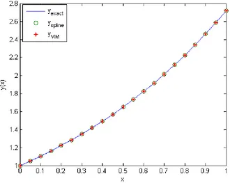
Figure 1, presents a comparison between the exact solution, yexact, the solution
ob-tained from the proposed method, yspline and the solution using the variational iteration
method, yVIM in the interval [0,1]. From figure 1, we can deduce that the proposed method provides excellent approximations to the solution of related equation to first or-der neutral delay differential equations. The numerical results showed that this method has very accuracy and reductions of the size of calculations compared with the VIM ([10], [12], [20], [21]).
Figure 1. Comparison between the exact solution and the solution obtained
6. Concluding remarks and discussion
This paper centralized to present a new method for solving the first order neutral delay differential equations. From the presented analysis shows that the proposed technique has much impact on the accuracy and efficiency of the solution on the first order neutral delay differential equations. We investigate the error estimation and the stability of the proposed method. The analytical approximation to the solutions is reliable, and confirms the power and ability of the proposed technique as an easy device for computing the solution of such these problems. Also, a comparison with the approximate method, variational iteration method is given. All computations in this paper are done using Matlab 7.1.
x m First app. sol. First absolute error Second app. sol. Second absolute error 0.1 1 1.10517091 3.5×10−09 1.10518247 1.1×10⁻⁵
2 1.10517091 1.3×10⁻¹⁰ 1.10518222 1.1×10⁻⁵
3 1.10517091 4.4×10⁻¹² 1.10518292 1.2×10⁻⁵
4 1.10517091 1.4×10⁻¹³ 1.10518299 1.2×10⁻⁵
5 1.10517091 4.7×10⁻¹⁵ 1.10518303 1.2×10⁻⁵ 0.2 1 1.22140275 7.8×10⁻⁹ 1.22141653 1.4×10⁻⁵ 2 1.22140273 2.1×10⁻⁸ 1.22141692 1.4×10⁻⁵
3 1.22140273 2.6×10⁻⁸ 1.22141710 1.4×10⁻⁵ 4 1.22140273 1.9×10⁻⁸ 1.22141727 1.4×10⁻⁵
5 1.22140274 1.0×10⁻⁸ 1.22141732 1.4×10⁻⁵
0.3 1 1.35774334 7.0×10⁻³ 1.35776052 7.9×10⁻³ 2 1.35308270 3.2×10⁻³ 1.35309976 3.2×10⁻³
3 1.35093385 1.0×10⁻³ 1.35095107 1.0×10⁻³
4 1.50144873 2.9×10⁻⁴ 1.35016221 3.0×10⁻⁴ 4 1.34991115 5.2×10⁻⁵ 1.34992858 6.9×10⁻⁴
0.4 1 1.50189327 1.0×10⁻² 1.50191342 1.0×10⁻²
2 1.49656938 4.7×10⁻³ 1.49658973 4.7×10⁻³ 3 1.49382185 1.9×10⁻³ 1.49384232 2.0×10⁻³
4 1.49125616 2.3×10⁻⁴ 1.49258221 7.6×10⁻⁴ 5 1.49205339 2.2×10⁻⁴ 1.49207150 2.5×10⁻⁴
0.5 1 1.66054058 1.1×10⁻² 1.66056441 1.7×10⁻²
2 1.65526313 6.5×10⁻³ 1.65528715 6.5×10⁻³
3 1.65195568 3.2×10⁻³ 1.65198099 3.2×10⁻³
4 1.65009713 1.3×10⁻³ 1.65012150 1.4×10⁻³
References
[1] A. Ayad, Spline approximation for second order Fredholm integro-differential equation, International Journal of Computer Mathematics, 66 (1997), 1-13.
[2] C. T. H. Baker, G. A. Bocharov and F. A. Rihan, Neutral delay differential equations in the modelling of cell growth, Journal of the Egyptian Mathematical Society, 16(2) (2008), 133-160.
[3] E. Boe and H. C. Chang, Dynamics of delayed systems under feedback control, Chem. Engng. Sci., 44 (1989), 1281-1294.
[4] R. K. Brayton and R. A. Willoughby, On the numerical integration of a symmetric system of difference-differential equations of neutral type, J. Math. Anal. Appl., 18 (1976), 182-189.
[5] D. R. Driver, A mixed neutral systems, Nonlinear Analysis: Theory Methods and Application, 8 (1984), 155-158.
[6] E. M. Elabbasy, T. S. Hassan and S. H. Saker, Oscillation criteria for first-order nonlinear neutral delay differential equations, Electronic Journal of Differential Equations, 134 (2005), 1-18.
[7] H. M. El-Hawary and K. A. El-Shami, Spline collocation methods for solving second order neutral delay differential equations, Int. J. Open Problems Compt. Math., 2(4) (2009), 536-545.
[8] D. J. Evans and K. R. Raslan, The Adomian decomposition method for solving delay differential equation,International Journal of Computer Mathematics, 10 (2004), 1-6.
[9] J. K. Hale, Theory of Functional Differential Equations, Springer-Verlag, New York, (1977). [10] J. H. He, Variational iteration method-a kind of non-linear analytical technique: some examples,
International Journal of Non-Linear Mechanics, 34 (1999), 699-708.
[11] M. M. Khader, On the numerical solutions for the fractional diffusion equation, Communications in Nonlinear Science and Numerical Simulations, 16 (2011), 2535-2542.
[12] M. M. Khader, Introducing an efficient modification of the variational iteration method by using Chebyshev polynomials, Accepted in Application and Applied Mathematics An International Jour-nal. To appear in 2012.
[13] E. Kreyszig, Introductory Functional Analysis with Applications, John Wiley and Sons, New York, (1989).
[14] I. Kubiaczyk, S. H. Saker and J. Morchalo, New oscillation criteria for first order nonlinear neutral delay differential equations, Applied Mathematics and Computation, 142 (2003), 225-242.
[15] G. Micula and A. Hayder, Numerical solutions of system of differential equations with deviating arguments by spline functions, Acta Tech. Napoca, 35 (1992), 107-116.
[17] M. A. Ramdan, Spline solution of first order delay differential equations, Journal Egyptian Mathe-matics Society, 1 (2005), 7-18.
[18] M. A. Ramdan and M. N. Shrif, Numerical solution of system of first order delay differential equations using spline functions, International Journal of Computer Mathematics, 83(12) (2006), 925-937. [19] V. Strygin, The spline-collocation method for a class of boundary value problems with deviating
arguments, Differential Equations, 33(7) (1998), 991-999.
[20] N. H. Sweilam and M. M. Khader, Variational iteration method for one dimensional nonlinear thermoelasticity, Chaos, Solitons and Fractals, 32 (2007), 145-149.