Bayesian random local clocks, or one rate to rule them all

R E S E A R C H A R T I C L E

Open Access

Bayesian random local clocks, or one rate to rule

them all

Alexei J Drummond

1,2*

, Marc A Suchard

3,4*

Abstract

Background:Relaxed molecular clock models allow divergence time dating and“relaxed phylogenetic”inference, in which a time tree is estimated in the face of unequal rates across lineages. We present a new method for relaxing the assumption of a strict molecular clock using Markov chain Monte Carlo to implement Bayesian modeling averaging over random local molecular clocks. The new method approaches the problem of rate variation among lineages by proposing a series of local molecular clocks, each extending over a subregion of the full phylogeny. Each branch in a phylogeny (subtending a clade) is a possible location for a change of rate from one local clock to a new one. Thus, including both the global molecular clock and the unconstrained model results, there are a total of 22n-2 possible rate models available for averaging with 1, 2, ..., 2n -2 different rate categories.

Results:We propose an efficient method to sample this model space while simultaneously estimating the

phylogeny. The new method conveniently allows a direct test of the strict molecular clock, in which one rate rules them all, against a large array of alternative local molecular clock models. We illustrate the method’s utility on three example data sets involving mammal, primate and influenza evolution. Finally, we explore methods to visualize the complex posterior distribution that results from inference under such models.

Conclusions:The examples suggest that large sequence datasets may only require a small number of local molecular clocks to reconcile their branch lengths with a time scale. All of the analyses described here are implemented in the open access software package BEAST 1.5.4 (http://beast-mcmc.googlecode.com/).

Background

In 1967, Allan Wilson and his then doctoral student Vincent Sarich described an “evolutionary clock” for albumin proteins and exploited the clock to date the common ancestor of humans and chimpanzees to five million years ago [1]. Given the limited informative-ness of these immunological data, this estimate has survived the intervening years remarkably well. This work was the first prominent application of the con-cept of a molecular clock [2] and, at the time, the result raised extreme controversy, as the commonly held belief advocated that the common ancestor of humans and African apes was much more ancient. In fact, previous authors had argued that there must have

been a slowdown of the rate of albumin evolution in African apes and humans to reconcile their great simi-larity with the presumed antiquity of their common ancestor.

Researchers have grappled with the tension between molecular and non-molecular evidence for evolutionary time scales ever since. Recently, a number of authors [3-7], have advanced“relaxed molecular clock”methods. These methods accommodate variation in the rate of molecular evolution from lineage to lineage. In addition to allowing non-clock-like relationships among sequences related by a phylogeny, modeling rate varia-tion among lineages in a gene tree also enable research-ers to incorporate multiple calibration points that may not be consistent with a strict molecular clock. These calibration points can be associated either with the internal nodes of the tree or the sampled sequences themselves. Furthermore, relaxed molecular clock mod-els appear to fit real data better than either a strict * Correspondence: [email protected]; [email protected]

1

Allan Wilson Centre for Molecular Ecology and Evolution, University of Auckland, Private Bag 92019, Auckland, New Zealand

3

Departments of Biomathematics and Human Genetics, David Geffen School of Medicine at UCLA, Los Angeles, CA 90095, USA

Full list of author information is available at the end of the article

molecular clock or the other extreme of no clock assumption [6]. In spite of these successes, controversy still remains around the particular assumptions underly-ing some of the popular relaxed molecular clock models currently employed. A number of authors [8-10], argue that changes in the rate of evolution do not necessarily occur smoothly nor on every branch of a gene tree. The alternative expounds that large subtrees share the same underlying rate of evolution and that any variation can be described entirely by the stochastic nature of the evo-lutionary process. These phylogenetic regions or sub-trees of rate homogeneity are separated by changes in the rate of evolution. This alternative model may be especially important for gene trees that have dense taxon sampling, in which case there are potentially many short closely related lineages amongst which there is not reason a priori to assume differences in the underlying rate of substitution.

Local molecular clocks are another alternative to the global molecular clock [11]. A local molecular clock per-mits different regions in the tree to have different rates, but within each region the rate must be the same. Up until now these models have been difficult to employ because their implementations did not permit the mod-eling of uncertainty in (1) the phylogenetic tree topology or (2) the phylogenetic positions of the rate changes between the local clock regions. For a model that allows one rate change on a rooted tree there are 2n − 2 branches on which the rate change can occur. To con-sider two rate changes, one must concon-sider (2n −2) × (2n −3) possible rate placements. If each branch can have 0 or 1 rate changes then the total number of local clock models that might be considered is 22n−2, where n is the number of sequences under study. For even moderate nthis number of local clock models can not be evaluated exhaustively.

In this paper we employ Markov chain Monte Carlo (MCMC) to investigate a Bayesian random local clock (RLC) model, in which all possible local clock configura-tions are nested. We implement our method in the BEAST 1.x [12] and BEAST 2 (http://code.google.com/ p/beast2/) open software frameworks. The resulting method co-estimates from the sequence data both the phylogenetic tree and the number, magnitude and loca-tion of rate changes along the tree. Our method samples a state space that includes the product of all 22n−2 pos-sible local clock models on all pospos-sible rooted trees. Because the RLC model includes the possibility of zero rate changes, it also serves to test whether one rate is sufficient to rule all the gene sequences at hand, as was Wilson and Sarich’s view of the African primate albumins.

Methods

Basic evolutionary model

We begin by considering data Y, consisting of aligned molecular sequences of length Sfromntaxa. We orien-tate these data such that we may writeY = (Y1, ...,YS), whereYsfor s= 1, ..., Sare the nhomologous charac-ters at each site sof the sequence alignment. To model this homology, we follow standard likelihood-based phy-logenetic reconstruction practice [13] and assume the data arise from an underlying continuous-time Markov chain (CTMC) process [14] along an unobserved treeτ. The treeτconsists of a rooted, bifurcating topology that characterizes the relatedness among the taxa, the gener-ally unknown historical times when lineages diverge in the topology and up to 2n−2 rate parameters rk that relate historical time and expected number of substitu-tions on each branch k. The CTMC process describes the relative rates at which different sequence characters change along the independent branches inτ. We restrict our attention in this paper to nucleotide substitution processes characterized by either the HKY85 [15] or GTR [16] infinitesimal rate matrices Λ and discrete-Gamma distributed across-site rate variation [17] with shape parameter a. However, our approach admits any standardly used CTMC for nucleotides, codons or amino acids.

LettingF= (Λ,a), we write the data sampling density of site s as P(Ys|τ, F). Felsenstein’s peeling/pruning algorithm [18] enables computational efficient calcula-tions ofP(Ys|τ,F). Assuming that sites are independent and identically distributed given (τ,F) yields the com-plete data likelihood

P P

S

s

s

Y| ,  Y | ,  .

(

)

=

(

)

=

∏

₁ (1)

Branch-specific rate variation

Model parameterization

We introduce the RLC model that allows for sparse, possibly large-scale changes while maintaining spatial correlation along the tree. We start at the unobserved branch leading to the most recent common ancestor (MRCA) of the tree and define the composite rate rMRCA= 1. Substitutions then occur on each branch k=

1, ..., 2n−2 below the MRCA with normalized rate

r c c

k k

k k

= × = × ×

( )

( ) _{( )} ,

 



_pa  (2)

where pa(k) refers to the parent branch above k, branch-specific rate multipliers= (1,...,2n-2) andc(·)

is a normalization constraint that ensures thatrkreflect the expected number of substitutions per unit time. This multiplicative structure on the compositerk=rpa(k)×k builds up a hierarchy of rate multipliers descending towards the tree’s tips.

Allowing all elements into vary independently leads to a completely non-clock-like model with, even worse, far too many free parameters for identifiability with the diver-gence times inτ. We avoid this problem through specify-ing a prior P() on the rate multipliers. This prior specifies that only a random numberKÎ{0,...,2n-2} ofk

≠1 such that rkdo not inherit their ancestors’ rate of change but instead mark the start of a new local clock, wherea prioriwe believeKis small. In effect, we place non-negligible prior probably onK= 0, the state in with one rate rules them all. Further, with mostrk=rpa(k), the

prior binds absolute rates equal on branches incident to the same divergence points.

Bayesian stochastic search variable selection

To infer which branch-specific rates rk do or do not inherit their ancestors’rate, we employ ideas from Baye-sian stochastic search variable selection (BSSVS) [21]. BSSVS traditionally applies to model selection problems in a linear regression framework. In this framework, the statistician starts with a large number of potential pre-dictors X1,...,XPand asks which among these associate linearly with anN-dimensional outcome variableY. For example, the full model becomesY = [X1,...,XP]b + , whereb is aP-dimensional vector of regression coeffi-cients andis anN-dimensional vector of normally dis-tributed errors with mean 0. When bp forp = 1,...,P differs significantly from 0,Xphelps predictY, otherwise Xpcontributes little additional information and warrants removal from the model via forcingbp=0. Given poten-tially high correlation between the predictors, determi-nistic model search strategies tend not to find the optimal set of predictors unless one explores all possible subsets. This exploration is generally computationally impractical as there exist 2P such subsets and comple-tely fails forP > N.

Recent work in BSSVS [22,23] efficiently performs the exploration in two steps. In the first step, the approach augments the model state-space with a set ofP binary indicator variables δ = (δ1,...,δP) and imposes a prior P(b) on the regression coefficients that has expectation 0and variance proportional to aP × Pdiagonal matrix with its entries equal to δ. IfδP= 0, then the prior var-iance on bpshrinks to 0 and enforces bp= 0 in the pos-terior. In the second step, MCMC explores the joint space of (δ,b) simultaneously.

To map BSSVS into the setting of rate variation, letδk be the binary indicator that a local clock starts along branchk, such that rk ≠rpa(k). Conversely, whenδk= 0, rk =rpa(k) implying thatk = 1. So, rate multipliers play an analogous role to the regression coefficients in BSSVS. An important difference is that kÎ [0,∞) and shrinks to 1, while bk Î(-∞,∞) and shrinks to 0, man-dating alternative prior formulations.

Prior specification

To specify a prior distribution overδ = (δ1,...,δ2n-2), we

assume that each indicator acts a priorias an indepen-dent Bernoulli random variable (RV) with small success probability c. The sum of independent Bernoulli RVs yields a Binomial distribution over their sum

K

_k k

n

=

∑

2₌−₁2



. In the limit thatK≪ c× (2n-2), this prior conveniently collapses to

K ~Truncated-Poisson( ), (3)

wherel is the prior expected number of rate changes along the tree τ. Choosingl = log2, for example, sets 50% prior probability on the hypothesis of no rate changes.

Completing the RLC prior specification, we assume that all rate multipliers in are a priori independent and

_k ~Gamma 1( /_k, /1 _k). (4)

Whenδk = 1, thena priori, k has expectation 1 and variance ψ, following in the vein of [24]. However, in light of BSSVS, whenδk= 0, the prior variance collapses to 0 andk= 1.

Normalization

To translate between the expected number of substitu-tionsbkon branchkand real clock-timetk,

bk = × × rk tk, (5)

Recall that we wish to measure μin terms of expected substitutions per unit real time, such that

 =

= −

= −

∑ ∑

b_k t

k n k k n 1 2 2 1 2 2 . (6)

To maintain this scaling, we sum Equation (5) over all branches and substitute the result into Equation (6). This eliminates the unknownμand yields

r t c t t

c t t

k k n k k k n k k k n k k k k k = − = − = −

∑

∑

∑

∑ ∑

= = = 1 2 2 1 2 2 1 2 2 ( ) , ( ) .     (7) Posterior simulation

We take a Bayesian approach to data analysis and draw inference under the RLC model via MCMC. MCMC straightforwardly generates random draws with first-order dependence through the construction of a Markov chain that explores the posterior distribution. Via the Ergodic Theorem, simple tabulation of a chain realiza-tion {θ(1),...,θ(L)} can provide adequate empirical esti-mates. To generate a Markov chain using the Metropolis-Hastings algorithm [25,26], one imagines starting at chain step ℓin state θ(ℓ)and randomly pro-posing a new stateθ* drawn from an arbitrary distribu-tion with density q(·|θ(ℓ)). This arbitrary distribution is commonly called a “transition kernel”. Finally the next chain stepℓ + 1 arrives in state

 

 

 

( ) min ,

( | ) ( ( )| )

( ( )| )

 



+1 ₌ 1 ×

  

with probability: P

P

q q

Y

Y (( | ( )) , . ( )       ⎧ ⎨ ⎪ ⎩⎪ ⎫ ⎬ ⎪ ⎭⎪ ⎧ ⎨ ⎪⎪ ⎩ ⎪ ⎪ otherwise (8)

The first term in the acceptance probability above is the ratio of posterior densities and the term involving the transition kernel is the Hastings ratio. The beauty of the algorithm is that the posterior densities only appear as a ratio so that intractable normalizing constant can-cels out.

Transition kernels

We employ standard phylogenetic transition kernels via a Metropolis-within-Gibbs scheme, as implemented in BEAST [12], to travel through most dimensions in the RLC parameter space. What is unique to the RLC model are transition kernels to explore rate multipliers and all possible local clock indicatorδconfigurations. Since kÎ [0,∞) we propose new rates * component-wise, such that for a uniform randomly selectedkwith

δk= 1,

_k _k

f U U s s f  ₌ ⎛ ⎝ ⎜ ⎜ ⎞ ⎠ ⎟ ⎟ ,

~Uniform , 1 , (9)

where 0< sf<1 is a tuning constant and the Hastings ratio is 1/U[27].

Transition kernels on δ are more challenging. One natural way to construct a Markov chain on a bit-vector state space, such as δ, involves selecting one random element δk with uniform probability 1/(2n − 2) and swapping its state _k _{= −}1 _k with probability 1 [14].

At first glance, the transition kernel densityq(δ*|δ) = q(δ|δ*) = 1/(2n - 2) appears symmetric leading to a Hastings ratio of 1. However, this view is flawed. One must recall that we introduced the indicators δ as a computational convenience. The number of different local clocksKover-shadowsδas our parameter of inter-est, upon which we place our truncated-Poisson prior P (K). The correct densities to calculate then become q (K*|K) and q(K|K*). Suppose the swapping event above generates 0 !1 so thatK* =K+ 1. AsKapproaches 0 the transition kernel finds it more and more difficult to decreaseKbecause the kernel is more likely initially to choose a 0 state for swapping. From this perspective, the kernel is definitely not symmetric in the interchange of K* and K. Assuming symmetry would lead to upwardly biased estimates forK< ⌊n- 1⌋. The reverse bias occurs asKapproaches 2n−2 from below.

To determine q(K*|K), we identify that our kernel chooses a δk= 0 with probability (2n−2−K)/(2n−2) and a δk = 1 with probabilityK/(2n −2). Therefore, if K* = K+ 1, q(K*|K) is the former probability and if K* =K- 1,q(K*|K) is the latter. Forming the Hastings ratio

q K K

q K K

K

n K K K

n K

K K K

( | ) ( | ) , .     = + − − = + − − + _{= −} ⎧ ⎨ ⎪⎪ ⎩ ⎪ ⎪ 1

2 2 1

2 2 1

1 if

if

(10)

This derivation provides an important lesson for those new to MCMC implementation; the Hastings ratio may vary depending on the model parameterization; it is, therefore, necessary to calculate the ratio as a function of the same parameterization as the prior.

In cases where the swap event relaxes the prior var-iance on the rate multiplierk, we simultaneously pro-pose a new value for _k _≠1. We draw this value from the prior given in Equation (4).

Model selection

Statistical inference divides into two intertwined approaches: parameter estimation and model selection. For the former, parameter inference relies on empirical estimates of P(θ|Y) that we tabulate from the MCMC draws. Model selection often represents a more formid-able task. The natural selection criterion in a Bayesian framework is the Bayes factor [28-30]. The Bayes factor B10in favor of ℳ1 overℳ0 is the ratio of the marginal

likelihoods ofℳ1andℳ0,

B P P P P P P 10 1 0 1 0 1 0 = ( | ) = ( | ) ( | ) ( | ) ( ) ( ), Y Y Y Y       (11)

and informs the phylogeneticist how she (he) should change her (his) prior belief P(ℳ1)/P(ℳ0) about the competing models in the face of the observed data. Involving the evaluation of two different normalizing constants, Bayes factors are often challenging to estimate.

By fortuitous construction, we side-step this computa-tional limitation when estimating the Bayes factor in favor of a global clock (GC) modelℳGCover the RLC modelℳRLC. ModelℳGCoccurs when K= 0, conveni-ently nested within modelℳRLC. Consequentially, theP (K= 0|ℳRLC) equals the prior probability ofℳGC, and P(K= 0|Y,ℳRLC) yieldsP(ℳGC|Y). Given this, a Bayes factor test ofℳGConly requires simulation under the RLC model. The Bayes factor in favor of a global clock

B P K

P K P K P K GC RLC RLC RLC RLC = = − = = − = ⎛ ⎝ ( | , ) ( | , ) ( | ) ( | ) 0 1 0 0 1 0 Y Y     ⎜⎜ ⎞ ⎠ ⎟ −1 . (12)

To calculate the ratio of marginal likelihoods we need only an estimator

_P

∧ of P(K=0|Y, ℳRLC). The Ergodic Theorem suggests that we let

P∧=

{

=

}

=

∑

1 0

1



 L

K( ) , (13)

where 1{·} is the indicator function. Occasionally

_P

∧ becomes a poor estimator when P(K = 0|Y,ℳRLC) decreases below or increases above 1 -for ≈ 1/L. In such situations, there are alternatives that depend on MCMC chains generated under several different prior probabilitiesP(K= 0|ℳRLC) [31]. The Bayes factor then provides the mechanism to combine results from the multiple chains and to rescale back to a believable prior.

Results

To explore the utility of the RLC model, we consider three well-studied examples that span the evolutionary scales from millions of years down to annual seasons. The first example investigates rate variation of several

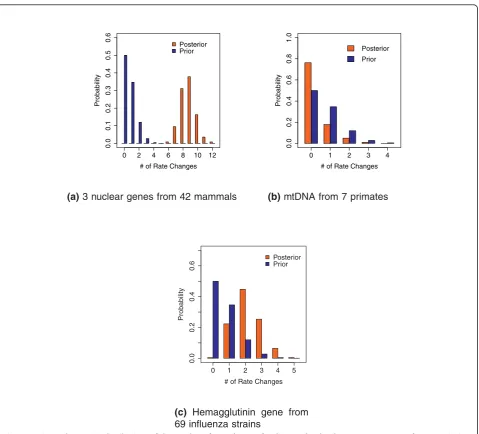
nuclear genes across the radiation of mammals [32]. Previous analyses fit these data under an unrooted phy-logenetic model, and then rely on post hoc heuristics while conditioning on the maximum likelihood tree to identify local molecular clocks. We exploit the RLC model to simultaneously infer both the tree and loca-tions of local clocks. We then turn our attention to mtDNA evolution within primates [33,34] and examine a subset of the original data in which multiple studies endorse a molecular clock [15,35,36] and demonstrate the ease in which one can formally test for a global clock via the RLC model. In both examples, the RLC model performs consistently with expectations. We con-clude with a survey of the temporal patterns of rate var-iation in hemagglutinin gene evolution and uncover a signature of multiple epochs of increasing rate without specifying prior knowledge of their existence.

Radiation of rodents and other mammals punctuated by local clocks

[32] investigate the existence of local molecular clocks during the radiation of mammals with an eye to recon-ciling molecular divergence dates with fossil evidence. In their study, [32] condition on a fixed evolutionary tree and perform multiple pair-wise or local rate heterogene-ity tests to construct an ad hocensemble of clock mod-els. We re-examine the same first and second codon positions of ADRA2B, IRBP and vWF nuclear genes (2422 alignment sites) from 42 mammals under the RLC model. Following [32], we assume the GTR model for nucleotide substitution with discrete-Γ site-to-site rate variation and ignore process heterogeneity across genes.

Figure 1 presents the Bayesian consensus tree for these data. Major groupings persist across tree esti-mates; examples include the marsupial/placental divide and major placental clades. Small topological differences are not surprising given data uncertainty and that researchers inferred the original tree under an unrooted model whereas our estimate is based on a local-clock-constrained model of phylogenetic trees.

Anthropoids’global clock

[33] and [34] present partial mtDNA sequences from nine primates, including two prosimians and seven anthropoids (monkeys/apes). The sequences comprise the protein coding regions for subunits 4 and 5 of the enzyme NADH-dehydrogenase and three tRNAs and contain 888 sites after the removal of alignment gaps. Since their publication, these data appear as molecular clock examples in several phylogenetic software releases [37-39]. [35,36] explore the strict molecular clock assumption in these data using a Bayesian approach and find good support for a clock among the anthropoids, but not between the anthropoids and pro-simians, nor within the prosimians. The Bayes factor tests developed in these former studies require compli-cated calculations that lend themselves poorly to

general use by evolutionary biologists. The RLC model provides a simple solution.

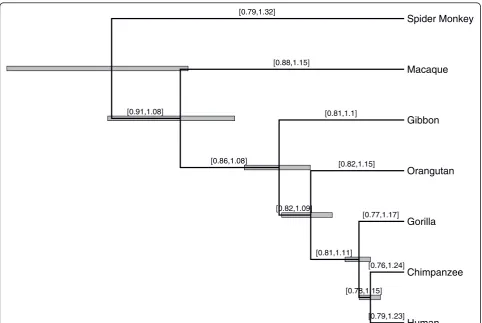
As an example in which a global clock should hold, we re-examine the seven anthropoids sequences under the RLC model. We employ the HKY85 [15] model for nucleotide substitution with discrete-Γ site-to-site rate variation. To keep exposition simple, we ignore struc-tured rate heterogeneity between the concatenated genes and across codon position with genes; however, these important modeling aspects remain straight-for-ward to include and do not complicate the final Bayes factor calculations. To complete specification, we assume l = log 2, such that there exists a 50% prior probability of a global clock.

Figure 3 presents the a posteriorimost probable tree relating these sequences. The topology of this tree

recapitulates the current paradigm of primate evolution, including the nearest-neighbor relationship between humans and chimpanzees, for which these data origin-ally helped settle [15,34]. We annotate the internal node heights in the figure with their posterior 95% Bayesian credible intervals (BCIs).

An important use of the molecular clock hypothesis is in estimating divergence times, and this ability remains under the RLC model. Near the tree branches in the fig-ure, we also report 95% BCIs for the branch-specific relative rates rk. Notably, all intervals cover the global clock hypothesized value of 1, suggesting the existence of a global clock in these data. However, these intervals

are univariate marginal reports of highly correlated ran-dom variables and multiple marginal assessments can lead to spurious conclusions. To test all branches simul-taneously, we calculate BGC from knowledge of the

model prior and an estimate

_P

∧ of the posterior prob-ability that number of rate changes K= 0. Figure 2(b) reports both the prior and estimate of the posterior probability mass function ofK. A majority of the poster-ior mass falls on K= 0, even more so than the prior. From the figure,BGC= 3.3. While this Bayes factor is

far from offering extreme support [28,29] for the global clock model itself, the balance of evidence favors a glo-bal clock over all other specific alternatives, and the

global clock would be contained in any credible set of models.

Temporal rate patterns in influenza

We examine hemagglutinin gene evolution from 69 strains of human influenza A [40]. These sequences represent serially sampled data; the earliest sequence stems from 1981 and the last from 1998, spanning a 17 year period. To infer the evolutionary tree and rate changes, we again employ the HKY85 model for nucleotide substitution, with Gamma-distributed rate heterogeneity among sites [24]. As priors, we assume an underlying coalescent process with a constant population size on the tree and a Poisson number of rate changes with an expected value of log2 [see Addi-tional file 2, for an example BEAST 1.5.4 XML script]. This specification places 50% prior probability on the strict molecular clock hypothesis.

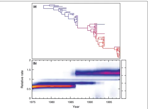
Figure 4(a) depicts the Bayesian consensus tree relat-ing these sequences, along with posterior mean branch lengths scaled in real time. To examine rate variation, we color branches by their posterior mean relative rate

of nucleotide substitution. Blue branches reflect the slowest rates of mutation through red branches that highlight regions of rapid change. From Figure 4(a), a general trend begins to take form of increasing rate var-iation over time; earlier branches to the left of the figure are mostly blue or purple, while late branches appear mostly red. We formally explore this trend in greater detail.

Figure 4(b) compares the posterior and prior mass functions relating the number of rate changes observed during hemagglutinin evolution. As expected from the observed variation in Figure 4(a), very little posterior mass falls on the existence of a global clock with zero rate changes. The modal number of rate changes is two. The Bayes factor rejecting a global clock is approxi-mately 45, providing strong support [28,29].

Figure 4(a) examines the heterogeneity of rate varia-tion as a process in time. To generate this plot, we dis-cretize time before the last sequence sampling date into 92 bins (four per year). For each bin, we construct the empirical posterior density of relative rates active along the tree during that time-period. Rates that we color

yellow or red occur with high posterior probability while rates proceeding towards white reflect lower probabil-ities. Consistent with the posterior mode of two rate changes shown in Figure 4(b), the two rate break-points in Figure 4(b) generate three distinct epochs in hemag-glutinin evolution, with a trend towards increasing rates over time. The first epoch begins at the root of the evo-lutionary tree and continues until some point between 1986 and 1992. The final epoch concludes with the 1998 strains.

We caution against over-interpretation of the punctu-ated form of the transitions between epochs seen in Fig-ure 4(b). While rate transitions may have arisen with such strong demarcation, their relative sharpness may be the result of the sampling pattern in this data set. The newer samples (between 1987 and 1998) are more densely sampled at each time point, while being sepa-rated by more time between samples (there are long

temporal breaks in strain sampling between 1987 and 1992 and again between 1994 and 1998). Temporal changes in sampling pattern could be particularly pro-blematic given the well accepted fact that the influenza virus population is subject to strong selection and the influenza data set used here has previously been shown to exhibit evidence for non-neutrality [40]. Richer taxon-sampling during the unsampled periods may clar-ify this issue, but remains beyond the scope of this methodological paper. Nonetheless, to confirm that the RLC model is performing appropriately, we do explore the temporal rate variation process in further detail using an explicitly temporal model of rate change. To do so these data were analyzed under a Bayesian imple-mentation (Andrew Rambaut pers comms) of a fixed-epoch model [41]. The result reinforces the conclusion that these data do exhibit temporal rate variation [see Additional file 1 for analysis summary and Additional

file 3 for the BEAST XML]. However, the fixed-epoch model requires a priorispecification of the number of different rate-epochs on which to fit the data, and assumes each rate change occurs simultaneously across all lineages, whereas the RLC assumes no such prior knowledge.

Discussion

Although it has been clear for quite some time that no universal molecular clock exists, a new question is emerging about what is the phylogenetic footprint of local molecular clocks. With increasing densely sampled phylogenetic trees, we should start to be able to get esti-mates of the extent of local clocks.

A major limitation of local clock models has been a dearth of methods to appraise all the possible rate assignments for various lineages [42]. BSSVS permits the efficient exploration of all 22n-2 possible local clock models and automatically returns the most parsimo-nious descriptions of the data.

The RLC description finds notable similarity to a com-pound Poisson process for rate variation [4]. Under this process, a Poisson number of change-points fall inde-pendently onto the branches of a phylogenetic tree. At each change-point, a Gamma-distributed random vari-able punctuates the current substitution rate. Without additional external information, the number of change-points (if greater than 1) and their specific locations along the branch are not identifiable by the likelihood, though this can be resolved by the prior. However this lack of identifiability places into question the benefit of allowing the large (in fact infinite) augmented state space of change points in the compound Poisson pro-cess that our BSSVS approach avoids. Under BSSVS, either there exists no change along a branch or there exists more than one and the new branch-specific rate represents an average over all events and their locations. BSSVS can also generalize to model heterogeneity in aspects of the CTMC process beyond rate variation. Examples we are considering include random local changes in nucleotide composition; a natural extension of previous work on modeling compositional heteroge-neity [43]. It is also possible to use this approach to model random local changes in parameters of the tree prior [44].

Compared to the auto-correlated rate models [3], the RLC approach imparts some different prior assumptions on rate variance among branches. For example, the prior variance on a lineage-specific rate depends on the number of internal nodes traversed between the root and branch, not the time-duration. Obviously, this fea-ture vanishes as the marginal prior on rates integrates over all possible trees. In the RLC model the number of traversed nodes reflects the number of sampled

speciation events a lineage has encountered. The evolu-tionary and sampling scenarios for which this serves as a better proxy for rate change than does time-duration is outside the scope of this work. Formal model testing can help settle this debate on a dataset-by-dataset basis. We have not attempted model comparison between the RLC and other relaxed clock models as part of this work, as it is a very challenging task. New methods for computing Bayes factors between non-nested phyloge-netic models, such as path sampling [45,46] and step-ping-stone sampling [47] may improve this situation in the future.

Further, hybrid models remain within reach in which rate multipliers draw a priorifrom a multivariate dis-tribution. The multivariate generalization of the Gamma is a Wishart, characterized by a scale matrix. This scale matrix could be a function of the time-tree.

While the transition kernels we employ in this paper successfully explore the posterior distribution for the three examples, we can envision datasets for which our algorithm would have difficulties producing accurate estimates of the posterior distribution. High correlation most likely exists between the evolutionary tree τ and location indicatorsδ alongτ at which local clocks start. Some datasets may possess posterior support for alter-native trees whose clock structures vary considerably. This situation poses a significant difficulty for our cur-rent transition kernels. These kernels alternate between updating τ with only small changesδ and updatingδ conditional onτ. In this construction, very rarely is it possible to make large moves in both tree-space and clock structures simultaneously, leading to potentially long mixing times. To remedy this, kernels that propose larger simultaneous jumps are warranted. While we are currently exploring different choices, finding kernels whose Hastings ratio remains convenient to calculate and function well across a range of datasets is proving challenging. We do, however, remain optimistic.

between indicators δ and rate multiplier; however, we believe this correlation strength is much smaller than between that above, as the multipliers only enter into the likelihood when δk= 1 and, hence, have consider-ably more freedom in their realized values. In any case, researchers should not blindly apply Bayesian samplers to new datasets; samplers require care and thought to ensure adequate exploration of the posterior parameter space.

Conclusions

We have proposed an efficient method to sample over random local molecular clocks while simultaneously estimating the phylogeny. The new method conveniently allows a comparison of the strict molecular clock against a large array of alternative local molecular clock models. We have illustrated the method’s utility on three exam-ple data sets involving mammal, primate and influenza evolution. We also explored a method to visualize the complex posterior distribution on the influenza data set which led to discovery of a strong temporal signal for the evolutionary rate in that data set, although this observation may well be attributed to temporal variation in sampling pattern. The examples that we have investi-gated suggest that large sequence datasets may only require a relatively small number of local molecular clocks to reconcile their branch lengths with a time scale. All of the analyses described here are implemen-ted in the open access software package BEAST 1.5.4 http://beast-mcmc.googlecode.com/.

Additional material

Additional file 1: Supplementary Information. This is a PDF file describing some additional details of the described methods including (i) a description of the proposal distribution for trees used in the RLC model and (ii) a summary of the analysis of the influenza data using a

“fixed epoch”model that allows the rate of evolution to change at a specific time in the past.

Additional file 2: Human.H3.81-98-local-gamma.xml. This is a BEAST XML input file compatible with BEAST 1.5.4 that implements the model combination used to analyze the influenza data set under the RLC model.

Additional file 3: Human.H3.81-98-2rate.xml. This is a BEAST XML input file compatible with BEAST 1.5.4 that implements the“fixed epoch” model used to confirm the signal for a temporal ate change in the influenza data set.

Acknowledgements

This paper was conceived in New Zealand, the new Middle Earth. We thank the Department of Computer Science, University of Auckland for hosting M. A.S. as an Honorary Research Fellow. We thank Andrew Rambaut for assisting with the fixed-epoch analysis of the Influenza data set. This work is supported in part by the John Simon Guggenheim Memorial Foundation, the National Evolutionary Synthesis Center (NSF #EF-0423641) and NIH R01 GM086887.

Author details

1_{Allan Wilson Centre for Molecular Ecology and Evolution, University of} Auckland, Private Bag 92019, Auckland, New Zealand.2Computational Evolution Group, University of Auckland, Private Bag 92019, Auckland, New Zealand.3_{Departments of Biomathematics and Human Genetics, David} Geffen School of Medicine at UCLA, Los Angeles, CA 90095, USA. 4_{Department of Biostatistics, UCLA School of Public Health, Los Angeles, CA} 90095, USA.

Authors’contributions

Both authors developed the idea and conducted the main experiments. AJD implemented the Bayesian stochastic search variable selection in the BEAST 1.5 and BEAST 2 open source software packages. Both authors debugged the software and wrote supporting software to analyze and visualize the results. Both authors were involved in the writing of the manuscript.

Received: 21 July 2010 Accepted: 31 August 2010 Published: 31 August 2010

References

1. Sarich VM, Wilson AC:Immunological time scale for hominid evolution.

Science1967,158:1200-1203.

2. Zuckerkandl E, Pauling L:Evolutionary Divergence and Convergence in ProteinsNew York: Academic Press 1965, 97-166.

3. Thorne JL, Kishino H, Painter IS:Estimating the rate of evolution of the rate of molecular evolution.Mol Biol Evol1998,15:1647-1657. 4. Huelsenbeck JP, Larget B, Swofford D:A compound poisson process for

relaxing the molecular clock.Genetics2000,154:1879-1892. 5. Sanderson MJ:Estimating absolute rates of molecular evolution and

divergence times: a penalized likelihood approach.Mol Biol Evol2002, 19:101-109.

6. Drummond AJ, Ho SYW, Phillips MJ, Rambaut A:Relaxed phylogenetics and dating with confidence.PLoS Biol2006,4:e88.

7. Rannala B, Yang Z:Inferring speciation times under an episodic molecular clock.Syst Biol2007,56:453-466.

8. Gillespie JH:Lineage effects and the index of dispersion of molecular evolution.Mol Biol Evol1989,6:636-647.

9. Gillespie JH:The Causes of Molecular EvolutionOxford: Oxford University Press 1991.

10. Bromham L, Penny D:The modern molecular clock.Nat Rev Genet2003, 4:216-224.

11. Yoder AD, Yang Z:Estimation of primate speciation dates using local molecular clocks.Mol Biol Evol2000,17:1081-1090.

12. Drummond AJ, Rambaut A:BEAST: Bayesian evolutionary analysis by sampling trees.BMC Evol Biol2007,7:214.

13. Felsenstein J:Inferring PhylogeniesSunderland, MA: Sinauer Associates, Inc 2004.

14. Lange K:Applied ProbabilityNew York: Springer 2003, [Springer Texts in Statistics.].

15. Hasegawa M, Kishino H, Yano T:Dating the human-ape splitting by a molecular clock of mitochondrial DNA.J Mol Evol1985,22:160-174. 16. Lanave C, Preparata G, Saccone C, Serio G:A new method for calculating

evolutionary substitution rates.J Mol Evol1984,20:86-93. 17. Yang Z:Among-site rate variation and its impact on phylogenetic

analyses.Trends Ecol Evol1996,11:367-372.

18. Felsenstein J:Evolutionary trees from DNA sequences: a maximum likelihood approach.J Mol Evol1981,17:368-376.

19. Kishino H, Thorne JL, Bruno WJ:Performance of a divergence time estimation method under a probabilistic model of rate evolution.Mol Biol Evol2001,18:352-361.

20. Thorne JL, Kishino H:Divergence time and evolutionary rate estimation with multilocus data.Syst Biol2002,51:689-702.

21. George EL, McCulloch RE:Variable selection via Gibbs sampling.J Am Stat Assoc1993,88:881-889.

22. Kuo L, Mallick B:Variable selection for regression models.Sankhya B1998, 60:65-81.

24. Yang Z:Maximum likelihood phylogenetic estimation from DNA sequences with variable rates over sites: approximate methods.J Mol Evol1994,39:306-314.

25. Metropolis N, Rosenbluth AW, Rosenbluth MN, Teller AH, Teller E:Equations of state calculations by fast computing machines.J Chem Phys1953, 21:1087-1092.

26. Hastings WK:Monte Carlo sampling methods using Markov chains and their applications.Biometrika1970,57:97-109.

27. Drummond AJ, Nicholls GK, Rodrigo AG, Solomon W:Estimating mutation parameters, population history and genealogy simultaneously from temporally spaced sequence data.Genetics2002,161:1307-1320. 28. Jeffreys H:Some tests of significance, treated by the theory of

probability.Proc Camb Philos Soc1935,31:203-222.

29. Jeffreys H:Theory of ProbabilityLondon: Oxford University Press, 1 1961. 30. Kass RE, Raftery AE:Bayes factors.J Am Stat Assoc1995,90:773-795. 31. Suchard MA, Weiss RE, Sinsheimer JS:Models for estimating Bayes factors

with applications in phylogeny and tests of monophyly.Biometrics2005, 61:665-673.

32. Douzery EJP, Delsuc P, Stanhope MJ, Huchon D:Local molecular clocks in three nuclear genes: divergence times for rodents and other mammals and incompatibility among fossil calibrations.J Mol Evol2003,57: S201-S213.

33. Brown WM, Prager EM, Wang A, Wilson AC:Mitochondrial DNA sequences of primates, tempo and mode of evolution.J Mol Evol1982,18:225-239. 34. Hayasaka K, Gojobori KT, Horai S:Molecular phylogeny and evolution of

primate mitochondrial DNA.Mol Biol Evol1988,5:626-644.

35. Suchard MA, Weiss RE, Sinsheimer JS:Bayesian selection of continuous-time Markov chain evolutionary models.Mol Biol Evol2001,18:1001-1013. 36. Suchard MA, Weiss RE, Sinsheimer JS:Testing a molecular clock without

an outgroup: derivations of induced priors on branch length restrictions in a Bayesian framework.Syst Biol2003,52:48-54.

37. Larget B, Simon DL:Markov chain Monte Carlo algorithms for the Bayesian analysis of phylogenetic trees.Mol Biol Evol1999,16:750-759. 38. Huelsenbeck JP, Ronquist F:Mrbayes: Bayesian inference of phylogenetic

trees.Bioinformatics2001,17:754-755.

39. Yang Z:PAML 4: a program package for phylogenetic analysis by maximum likelihood.Mol Biol Evol2007,24:1586-1591.

40. Drummond AJ, Suchard MA:Fully Bayesian tests of neutrality using genealogical summary statistics.BMC Genet2008,9:68.

41. Drummond A, Forsberg R, Rodrigo AG:The inference of stepwise changes in substitution rates using serial sequence samples.Mol Biol Evol2001, 18:1365-1371.

42. Sanderson MJ:A nonparametric approach to estimating divergence times in the absence of rate consistency.Mol Biol Evol1997, 14:1218-1231.

43. Foster PG:Modeling compositional heterogeneity.Syst Biol2004, 53:485-495.

44. Gray RD, Drummond AJ, Greenhill SJ:Language phylogenies reveal expansion pulses and pauses in pacific settlement.Science2009, 323:479-483.

45. Lartillot N, Philippe H:Computing Bayes factors using thermodynamic integration.Syst Biol2006,55:195-207.

46. Beerli P, Palczewski M:Unified framework to evaluate panmixia and migration direction among multiple sampling locations.Genetics2010, 185:313-326.

47. Fan Y, Wu R, Chen M-H, Kuo L, Lewis PO:Choosing among partition models in Bayesian phylogenetics.Mol Biol Evol2010.

48. Liu JS:The collasped Gibbs sampler in Bayesian computations with applications to a gene regulation problem.J Am Stat Assoc1994, 89:958-966.

49. Redelings BD, Suchard MA:Joint Bayesian estimation of alignment and phylogeny.Syst Biol2005,54:401-418.

doi:10.1186/1741-7007-8-114

Cite this article as:Drummond and Suchard:Bayesian random local clocks, or one rate to rule them all.BMC Biology20108:114.

Submit your next manuscript to BioMed Central and take full advantage of:

• Convenient online submission

• Thorough peer review

• No space constraints or color figure charges

• Immediate publication on acceptance

• Inclusion in PubMed, CAS, Scopus and Google Scholar

• Research which is freely available for redistribution