University of New Orleans University of New Orleans
ScholarWorks@UNO
ScholarWorks@UNO
University of New Orleans Theses and
Dissertations Dissertations and Theses
Spring 5-13-2016
A study of three paradigms for storing geospatial data:
A study of three paradigms for storing geospatial data:
distributed-cloud model, relational database, and indexed flat file
distributed-cloud model, relational database, and indexed flat file
Matthew A. Toups
University of New Orleans, [email protected]
Follow this and additional works at: https://scholarworks.uno.edu/td
Part of the Databases and Information Systems Commons, and the Data Storage Systems Commons
Recommended Citation Recommended Citation
Toups, Matthew A., "A study of three paradigms for storing geospatial data: distributed-cloud model, relational database, and indexed flat file" (2016). University of New Orleans Theses and Dissertations. 2196.
https://scholarworks.uno.edu/td/2196
This Thesis is protected by copyright and/or related rights. It has been brought to you by ScholarWorks@UNO with permission from the rights-holder(s). You are free to use this Thesis in any way that is permitted by the copyright and related rights legislation that applies to your use. For other uses you need to obtain permission from the rights-holder(s) directly, unless additional rights are indicated by a Creative Commons license in the record and/or on the work itself.
A study of three paradigms for storing geospatial data: distributed-cloud model, relational database, and indexed flat file
A Thesis
Submitted to the Graduate Faculty of the University of New Orleans in partial fulfillment of the requirements of the degree of
Master of Science in
Computer Science
by Matthew Toups
Acknowledgments
I must express my deep gratitude to Dr. Elias Ioup and Dr. Mahdi Abdelguerfi who not only supported me during this work, but without whom my studies in this program would not be pos-sible. I additionally thank Dr. Shengru Tu and Dr. Md Tamjidul Hoque for their service on my thesis committee.
Finally, I thank my mother, Merry Toups, for her support throughout.
Contents
List of Figures... v
List of Tables... v
Abstract... vi
1 Introduction... 1
2 Background... 2
2.1 Open Geospatial Consortium data model and services... 2
2.2 Spatial data in a Relational database... 3
2.2.1 PostgreSQL... 3
2.2.2 PostGIS... 4
2.3 Spatial data in an indexed flat file ... 4
2.3.1 Vector Cluster History ... 4
2.3.2 Vector Cluster Format... 6
2.3.3 GeoPackage ... 6
2.4 Spatial data in a distributed-cloud key-value store ... 6
2.4.1 Distributed computing framework: Hadoop... 7
2.4.2 Key-value store: Accumulo ... 8
2.4.3 Spatiotemporal index: GeoMesa ... 8
2.4.4 Other approaches to geospatial computing on Hadoop ... 9
2.5 The OpenStreetMap dataset ... 9
2.6 Privacy and Security in geospatial data... 10
3 Methodology... 11
3.1 Configuration and deployment of Geospatial data services... 11
3.1.1 Vector Cluster ... 11
3.1.2 GeoMesa/Accumulo/Hadoop platform ... 11
3.1.3 PostgreSQL/PostGIS server ... 12
3.2 Building data stores... 13
3.2.1 Generating a Vector Cluster file ... 13
3.2.2 Ingestion into GeoMesa... 13
3.2.3 Insertion into PostgreSQL ... 14
3.3 Early Experiments... 15
3.4 Refined experimental design ... 16
3.5 Measurements ... 17
3.6 Simulating tile server workload using randomly chosen bounding boxes... 17
3.6.1 Within contiguous North America (all-layer tests) ... 18
3.6.2 Within feature-dense areas (single-layer tests)... 19
3.7 Testing with multithreading (all-layer tests) ... 19
3.8 Hardware ... 20
4.1 Generalized performance comparison ... 21
4.2 Which parameters impact query performance ... 21
4.2.1 Size of area to be queried ... 22
4.2.2 Number of objects returned ... 24
4.3 Parallelism... 27
5 Conclusions... 30
5.1 Implications for cloud-based geospatial data infrastructure ... 31
5.2 When is a problem a “big data” problem? ... 32
5.3 Future work ... 33
6 References... 34
List of Figures
1 Early testing apparatus . . . 16
2 Refined testing apparatus . . . 17
3 Example of building a tile from queries of many layers . . . 18
4 Randomly generated bounding boxes across continental North America . . . 19
5 Randomly generated bounding boxes in and around San Jose, California . . . 20
6 GeoMesa: query times for varying size bboxes (San Jose highway layer) . . . 23
7 PostGIS: query times for varying size bboxes (San Jose highway layer) . . . 23
8 Vector Cluster: query times for varying size bboxes (San Jose highway layer) . . . 24
9 GeoMesa: query times for varying object densities (San Jose highway layer) . . . . 25
10 PostGIS: query times for varying object densities (San Jose highway layer) . . . 25
11 Vector Cluster: query times for varying object densities (San Jose highway layer) . 26 12 All 3 services, compared . . . 26
13 Vector Cluster threading results histogram (all layers) . . . 28
14 PostGIS threading results histogram (all layers) . . . 28
15 GeoMesa threading results histogram (all layers) . . . 29
List of Tables
1 Accumulo’s key/value structure[15] . . . 82 Software versions used for cluster infrastructure . . . 12
3 Service distribution across the available hardware nodes . . . 12
4 SimpleFeatureType schema used in GeoMesa . . . 14
5 Experimental hardware . . . 21
6 Overall performance comparison: North America bboxes, full tile (all layers), 7 threads . . . 21
7 Summary of storage backends and their properties . . . 30
Abstract
Geographic Information Systems (GIS) and related applications of geospatial data were once a small software niche; today nearly all Internet and mobile users utilize some sort of mapping or location-aware software. This widespread use reaches beyond mere consumption of geodata; projects like OpenStreetMap (OSM) represent a new source of geodata production, sometimes dubbed “Volunteered Geographic Information.” The volume of geodata produced and the user demand for geodata will surely continue to grow, so the storage and query techniques for geospatial data must evolve accordingly.
This thesis compares three paradigms for systems that manage vector data. Over the past few decades these methodologies have fallen in and out of favor. Today, some are considered new and experimental (distributed), others nearly forgotten (flat file), and others are the workhorse of present-day GIS (relational database). Each is well-suited to some use cases, and poorly-suited to others. This thesis investigates exemplars of each paradigm.
Keywords:
1
Introduction
The reach and importance of Geographic Information Systems (GIS) have grown since the 1980s, from a niche software market for a few groups of professionals, to a widely-used technology present on almost any Internet-connected computer or mobile device. Access to the technology for both creating and consuming GIS data and related content has made these systems and the data that they process a part of daily life.
One way that both the creation of use of geospatial data has changed has been the advent and growth of Volunteered Geographic Information (VGI)[18]. The largest and best-known example of this is the OpenStreetMap (OSM) dataset, which is both generated by and available to the public, and is used as raw data for these experiments.
The work presented here will consider the data that powers GIS, in particular, vector data. What this data is, how it is structured, and three fundamentally different ways of processing it will be detailed in Section 2. These methods, orparadigms, span a wide range of topics in computing. The simplest is the flat file, indexed for spatial searches but stored simply on a single filesystem and accessed using a simple API. The most complex (and newest) is the distributed-cloud key-value store, built atop many levels of software platforms and a possibly large amount of computing hardware. Somewhere in between these, and a longtime player in geospatial computing, is the
relational database, a powerful tool for managing many types of data. One exemplar of each type is selected and described; brief information on other forms not tested here is also provided.
Section 3 details the process used to deploy these three systems, and how testing was performed in the early part of this investigation. Based on lessons from the initial tests, a more rigorous experimental design is presented, along with three different types of measurements to apply to each of the three exemplar systems.
Section 4 presents the results of these tests, from a broad generalized comparison of the three systems, to more specific questions about what types of queries yield what results, and how they behave under a simulated load of parallel requests.
Finally, Section 5 summarizes the advantages and disadvantages of each system, relates these to their respective design choices and philosophies, and comments on future directions for work on this topic.
2
Background
This thesis is concerned with vector data, often contrasted with raster(or bitmap) data. Raster data typically (but not necessarily) consists of a 2-dimensional image suitable for human viewing. Vector data is not an image, but a geometric representation of a spatial feature; the most common examples of geometric primitives would be a point, a line, and a polygon. Vector data requires less space to store than raster data, but often requires more processing in order to be used in a GIS application. [32, pp. 35,193]
Uses of this data include visualizing in a desktop GIS application, display in a web-based application, or more complex analysis of geospatial data such as routing. As GIS applications become increasingly web-based, vector data management has followed. The flat files of vector data used in desktop GIS are typically replaced by relational databases in web applications. According to Sample and Ioup,
There are two primary methods of storing vector data for tiling: database storage and file system storage. Database storage of vector data is more common than file storage when the data is to be retrieved using geospatial queries. File storage is more commonly used for archival and distribution of vector data as fixed data sets. [32, p. 196]
The newer distributed-cloud key-value stores introduced in recent years1could also be considered a type of “database” storage within that dichotomy, but since they introduce many new advantages and disadvantages, the distributed-cloud model will be considered a distinct third paradigm here.
The authors go on to describe a file format which, perhaps counter-intuitively, achieves some of the index and query advantages of a database. This idea would become the Vector Cluster format, detailed in Section 2.3.
Prior to that, in the following two sub-sections, the OGC data model and a common implemen-tation of it, PostGIS, will be described.
Later in this section, the recently popular distributed-cloud approaches will be described, with a focus on GeoMesa. Then, more information is presented on the OSM data set, and finally the growing need for privacy and security features in geospatial data storage systems.
2.1
Open Geospatial Consortium data model and services
Much recent work in geospatial computing utilizes some part of the standards defined by the Open Geospatial Consortium (OGC), from basic data models and types (such as Simple Features) to file formats/markup languages (such as KML2) to widely-used publishing services (such as WMS,
WMTS, WFS, WPS3) and others.
The OGC defines open standards for data and services to ensure “geospatial interoperability”. With this goal in mind, the OGC standards organization began as a collaboration of government, 1At the time of [32]’s publication in 2010, new distributed-cloud frameworks did yet not support geospatial data,
so that work only addresses Hadoop as an ill-suited platform for processing raster tiles, not vector data; that would be made possible by the advent of GeoMesa and similar systems in later years.
2KML stands for Keyhole Markup Language, popularized by Google Earth, a software package purchased by
Google in 2004 and subsequently distributed at no charge on the Internet.
academic, and private-sector members of the GIS community in the early 1990s. Much of the effort’s origins can be traced farther back to the GRASS GIS community which grew around the seminal GRASS (Geographic Resources Analysis Support System) software suite created by the U.S. Army Corps of Engineers in the early 1980s.[8]
The OGC standard of interest in this work is the Simple Feature, a model for the storage and access of geographic information. [7] This industry standard went on to become an international standard: ISO 19125. [23] The standard outlines a model for storing geometries, attributes, and spatial reference systems, specifying names and types for data. Both GeoMesa and PostGIS im-plement this standard. Vector Cluster does not.
Software described herein uses the Java implementation of the SimpleFeature4and other standards from OGC’s Geotools version 11.2. OGC standards also provide standardized abstrac-tions for common access methods and types, such asDataStore,FeatureStore, andQuery.
2.2
Spatial data in a Relational database
Before considering two radically diverging paradigms for geospatial data storage (flat files and distributed key-value cluster), it is worth examining what could be considered a middle ground: the relational database (or RDBMS). This is certainly the most widely used of the three methods considered, and therefore is well studied.
Two components together make up the RDBMS geodata software which will be tested: Post-greSQL, a very well known and mature general-purpose RDBMS; and PostGIS, an extension for geospatial data.
Other relational databases support spatial indexes and queries. Oracle has produced a spatial option for its relational database since the 1990s, known as “Spatial Data Option”, then “Oracle Spatial”, and most recently “Oracle Spatial and Graph”. More recently, MySQL added extensions for spatial data, following the OGC specitications, but this is not a mature or widely-used system. Only PostgreSQL/PostGIS will be tested here.
2.2.1 PostgreSQL
PostgreSQL is used here as exemplar of a traditional relational database. Created in 1986 by Stonebraker at the University of California at Berkeley (UCB), PostgreSQL is the successor to Ingres[35] (implemented in 1975-1977, also at UCB) and has been widely influential in the design of relational databases.
PostgreSQL has traditionally been used as a single-node database server, serving requests from one or many clients. These clients may be software running on the same host, or connecting from other systems over a network.
PostgreSQL does have some support for clustering, but this is usually in the form of sim-ple replication for the purposes of load balancing and high availability.[10] Historically the Post-greSQL project policy was to avoid supporting replication in the core of the database, and instead to encourage third parties to develop competing approaches as add-ons. But starting in 2008, the PostgreSQL core team did introduce simple replication support into the core project. [24]
2.2.2 PostGIS
PostGIS is an extension to PostgreSQL which adds support for geospatial data and analysis.[6] It is an open-source project under the Open Source Geospatial Foundation [36] (OSGeo) and inde-pendent from the PostgreSQL project. Despite yet another similar name, OSGeo is distinct and unrelated to OGC and OSM. However each of these organizations contribute to the same ecosys-tem of Free Open Source Software for Geospatial (FOSS4G), which is also the name of an annual conference organized by OSGeo.[28]
PostGIS uses the standard OGC Simple Features for GIS objects5as well as functions that op-erate over them, and OGC-compliant metadata on Spatial Reference Systems (SRS). The PostGIS spatial index is an R-tree over GiST (Generalized Search Tree). [6]
2.3
Spatial data in an indexed flat file
The oldest method of storing geospatial data is the simple “flat” file. In this context, a flat file is not necessarily devoid of any structure, but is distinguished by the following properties:
• consists of a single file (can be easily transferred)
• accessible through standard filesystem operations (and stored on virtually any device)
• does not require a server or other software devoted solely to handling requests
Strong proponents of relational databases may consider the flat file to be an obsolete idea, but some recently created geospatial data file types challenge that notion: Vector Cluster, and GeoPackage. They both push the boundaries of the notion “flat” by utilizing features from rela-tional databases (especially spatial indexes), but still meet the three criteria given above. Perhaps geospatial data has come full circle and returned to consider the flat file again.
The newer format, GeoPackage, will be described briefly in Section 2.3.3; Vector Cluster will be examined with more detail, and will be used for the experiments in this work.
2.3.1 Vector Cluster History
Vector Cluster is a geospatial data storage format created by the Geospatial Computing Section at the United States Naval Research Laboratory (NRL). NRL’s products require large amounts of vector data with fast access times in order to support real-time on-the-fly generation of WMS tiles based on many data sources. [22]
Prior to the creation of Vector Cluster, many government projects stored vector data in a for-mat called Vector Product Forfor-mat (VPF). This forfor-mat was developed by the National Geospatial-intelligence Agency (NGA) (previously known as National Imagery and Mapping Agency, and prior to that known as Defense Mapping Agency) in the late 1980s, and was later adopted into the Digital Geographic Exchange Standard (DIGEST) standard.[4] [3]
NRL researchers discovered that VPF was an unsuitable format for the modern, dynamic GIS system they were building. In order to render raster tiles on-demand from vector data, random-access queries must be practical. VPF had no support for geospatial queries and indices, a major 5Technically PostGIS implements a superset of the OGC Simple Features; PostGIS developers extended the model
limitation. This means that, for example, in order to find objects that match a certain bounding box, every object must be scanned and compared to the bounding box. So any search required a full scan, greatly limiting the scalability of any GIS service.
At the time that NRL hit this limitation in the late 2000s, they also found the query performance for geospatial data in relational databases to be poor. More importantly, NRL needed a file format without the additional requirements of an RDBMS.
Vector Cluster was born from this need, and derives its name from another NRL product, the Tile Cluster6. A Vector Cluster consists of a single flat file with a format further detailed in Section
2.3.2.
The Vector Cluster format is notable for its simplicity, from which it derives much of its advan-tages. The format is also much more limited in what it supports, compared to other data storage approaches, as it was tailored to solve a narrowly defined problem.
NRL Geospatial Computing needed a way for clients to query a large set of vector data to dy-namically generate maps on demand. These clients may not be strongly connected to a network, for example those in underwater craft. The client programs may also be running on smaller sys-tems, such as those running the Android mobile operating system. Vector Cluster supports these use cases.
Vector Cluster does not support many other features that would be expected in something like a database. Vector Clusters can not edit or delete records, it is essentially a read-only format7. Updates to map data are performed periodically by regenerating the vector cluster entirely. One example given is the Digital Nautical Chart (DNC) data, from which a new Vector Cluster is generated every two weeks. [22]
Vector Cluster has its own complete API for vector geometries, features, queries, and more. It does not use any of OGC’s GeoAPI, but implements much of the functionality independently. One difference is that OGC Simple Feature uses a fixed attribute schema, whereas NRL’s Feature type can be schema-less. Other than that difference, much of the Vector Cluster API duplicates OGC’s GeoAPI.
The proponents of Vector Cluster’s simple flat-file design argue that the guarantees commonly provided by relational databases (atomicity, consistency, isolation, and durability) and related fea-tures (locking, rollbacks) are not useful for geospatial vector data when generating map tiles. By eliminating these features, the goal is to achieve a more efficiency for the more frequent use: read-ing data usread-ing a spatial query.[32]
The Vector Cluster format is in production use in several government contexts. The public Geospatial Computing Tile Server8 uses vector clusters as its vector data source when rendering tiles. [22]
6The tile cluster is also a flat-file approach, but for storing raster tile data. It is designed to work around filesystem
limitations with regard to many small files.
7Robert Owens of NRL says that it would be possible to add edit/delete support to the Vector Cluster library, but
this has never been implemented.
8
2.3.2 Vector Cluster Format
While a Vector Cluster is a single file, it is well-structured and indexed for efficient access.9 A Vector Cluster can contain one or many feature layers, which can be found quickly by way of a B+ Tree index on the layers.
Each layer has its own header and is independently indexed. The spatial index is a 2-dimensional R* Tree. Accordingly, nodes in the tree are ordered by Minimum Bounding Rectangle (MBR). The Vector Cluster can support attributes with a schema, or use a schema-less key/value pair system. [22]
2.3.3 GeoPackage
GeoPackage (defined by OGC in 2014) is a newer file format with very similar goals to Vector Cluster. It aims to provide a single file suitable for disconnected mobile devices, and as an inter-change format in a heterogenous software environment. GeoPackage is “serverless”, with clients accessing the file directly (using a software library). And like Vector Cluster, it also uses an R Tree as a spatial index. [27]
One notable difference is that, despite the simple single-file, serverless model, GeoPackage does consider itself an RDBMS with the transactional guarantees that typically carries:
all changes to data in the container are Atomic, Consistent, Isolated, and Durable (ACID) despite program crashes, operating system crashes, and power failures. [27] These are the same guarantees eschewed by the Vector Cluster designers.
It may seem surprising at first: a simple file format which also promises database-level guar-antees and accessibility. It turns out GeoPackage is based on a non-geospatial file format which provides both of these things: SQLite. It may not be as conspicuous as PostgreSQL, but SQLite is actually used more broadly. Its creators make a convincing argument that it is “Most Widely Deployed and Used Database Engine”, due to its common use as a configuration file format in widely used10 software such as the browsers Firefox, Chrome and Safari and even the operating
systems Windows 10, Mac OS, and Android.[34]
This new file format is quite promising and is being widely adopted, from the open-source library GDAL, to commercial ArcGIS suite from Esri, to government software from the National Geospatial-Intelligence Agency (NGA). GeoPackage supports both vector and raster data.
Flat-file purists may not be enamored with GeoPackage due to its use of SQLite, but it delivers the desired flat-file features: single file, serverless, indexed; and unlike Vector Cluster, GeoPackage is cross-platform compatible with many types of GIS software. The performance of GeoPackage is not yet well studied, however, and will not be tested in this work.
2.4
Spatial data in a distributed-cloud key-value store
The advent and publication of the Google File System [16] (GFS) in 2003 and the related MapRe-duce computation model[9] in 2004 has inspired the development of distributed systems and large 9Arguably the index means the file is no longer “flat” — but it is still far simpler than the other methods studied,
so relatively speaking, “flat” (as the term is used here) would still apply.
10This remarkably wide use is made possible because SQLite is dedicated to the public domain and can be embedded
scale computation frameworks which are now used widely. The most prominent project inspired by those publications is Hadoop [17], an open-source software framework under the Apache Software Foundation, with major contributions from engineers at Yahoo Inc.11 and other large web-based
organizations. Although research papers describing the software have been released to the public, GFS and MapReduce12 are proprietary software not available outside of Google13. Hadoop and
related projects are open-source and freely available, so despite being a later arrival, they see more use in both research and production.
Many “big data” oriented efforts utilize the Hadoop framework. Many software systems have been built atop the Hadoop framework, most of which will not be named here. Two prominent examples are Hive, a data warehouse system, and HBase, a distributed key-value store. HBase has been used in some geospatial computing work, but will not be used here.
The Hadoop-based datastore used in this work is Accumulo, which is extended for spatio-temporal data by GeoMesa. These will each be detailed in this section. First, the layer which lies under these systems, Hadoop, will be described.
2.4.1 Distributed computing framework: Hadoop
At it’s simplest, Hadoop can be broken down into two key components: HDFS and YARN (a MapReduce implementation).
HDFS is the Hadoop Filesystem, a distributed filesystem over many nodes, which provides fault tolerance, parallel access and load balancing. HDFS is closely paired with the MapReduce framework (the 2nd generation of which is called YARN). This tight relationship between dis-tributed data storage and disdis-tributed computational power lies at the core of Hadoop’s large-scale data analytics design.
When building distributed systems at a large enough scale, hardware failures become a regular occurrence and must be accounted for in the system design. The GFS design (and thus Hadoop) have built-in redundancy as well as the ability to add and remove nodes dynamically.
While it is possible for HDFS and YARN to run on a single computer, doing so negates any benefits the distributed-computing framework offers and is only done for testing purposes. At their core, HDFS and YARN are designed to run on a large number of (possibly low-cost, commodity) computers, referred to as “nodes”. Some of these nodes include:
• Name Nodes, which manage and provide HDFS filesystem metadata
• Data Nodes, which store HDFS data blocks
• Yet Another Resource Negotiator (YARN): tracks resources and orchestrates work (such as MapReduce jobs) across many nodes
• Zookeeper (similar to the Paxos algorithm): manages configuration, naming, and provides synchronization
11Yahoo and Google are both Internet advertising firms based in California.
12Originally MapReduce referred to Google’s proprietary implementation, but now the term is used generically to
refer to computation using that model.
2.4.2 Key-value store: Accumulo
Accumulo is a distributed key-value datastore based on the BigTable design from Google [33]. As with GFS and MapReduce mentioned above, the publication of the BigTable paper [5] describes proprietary software available only within Google, but has spurred new developments in open source software, especially those under the Apache Software Foundation.
An Apache project since 2011, Accumulo splits tables up into “tablets” of contiguous, sorted rows which are stored in HDFS, which provides data redundancy and high throughput I/O. [33] Accumulo also extends the BigTable design in two significant ways:
• Column visibility: this optional value restricts access to each individual cell based on the authentication tokens specified. Using this value, Accumulo can offer fine-grained data se-curity/privacy capabilities with this cell-level security label.[14]
• Iterators: similar to reducers in MapReduce frameworks, iterators allow for server-side pro-cessing. They are typically used to filter and transform data, possibly chained or in parallel across many tablet servers [33] [15]
Accumulo’s multidimensional key includes the visibility feature for security, as well as various other fields. Table 1 shows this unique key format, which offers notable advantages. In addition to the fine-grained access-controls, the timestamp value in the key allows for temporal filtering on the server side using iterators.
Key
Value Row ID Column Family Column Qualifier Column Visibility Timestamp
Table 1: Accumulo’s key/value structure[15]
Unlike searches on a relational database, which can utilize the index from multiple columns to expedite results, in a “NoSQL”14key/value store such as Accumulo, only one index is built on the lexicographically-ordered records.
2.4.3 Spatiotemporal index: GeoMesa
GeoMesa enables indexing and querying of spatiotemporal data on Accumulo, similar to the rela-tionship between PostGIS and PostgreSQL. Like PostGIS, GeoMesa is not a standalone piece of software, but a library added-on to Accumulo15to enable support for spatiotemporal data.
GeoMesa uses and extends the OGC SimpleFeature data model and supports spatiotemporal indexing (within Accumulo’s single key) by interleaving a record’s geometry with its associated datetime string. This index is then split up between the three components of Accumulo’s key structure: Row ID, Column Family, and Column Qualifier (as shown in Table 1). [15]
14This term originally referred to non-relational databases, but more recently has been associated with the phrase
“not only SQL”.
15GeoMesa is designed to work on other key/value stores such as HBase. But Accumulo is best supported; support
2.4.4 Other approaches to geospatial computing on Hadoop
GeoMesa is but one of many approaches to spatial data indexing on the Hadoop framework. Whit-man et al. reviewed GeoMesa and other Hadoop-based spatial data approaches before proceeding with implementing a Point Matrix Region (PMR) quadtree index with support for range and k nearest node (k-NN) spatial queries. GeoMesa does not support k-NN queries. Whitman et al.’s implementation does not use Accumulo to split and store data, but uses a MapReduce job to build the quadtree. One advantage they claim is that a MapReduce job is notrequired for access, pro-viding “efficient, random-access queries” because “neither a full table scan, nor any MapReduce overhead is incurred when searching”.[39]
Hadoop-GIS/RESQUE [1] is built on Hive, a Hadoop-based package supporting SQL-like queries on spatial data, as opposed to Accumulo’s NoSQL key/value approach. Hadoop-GIS was motivated by medical imaging uses, supports range and self-join queries, and employs an R*-tree. SpatialHadoop is built on Hadoop MapReduce, uses R+ tree indexing, and supports range, k-NN, and more computational geometry operations. Unlike Whitman et al.’s approach, Spatial-Hadoop does require a MapReduce job for each query. Eldawy and Mokbel’s work includes a MapReduce extractor for OpenStreetMap data. [12]
2.5
The OpenStreetMap dataset
OpenStreetMap16 (OSM) is a notable project that collects, stores, and displays map data con-tributed by users (“crowd-sourced”).[19] Founded in 2004 in the UK, OSM’s mission is to create map data available to all under a Free and Open license, powered by free software and by a com-munity of volunteer editors. It has grown into a complete and vibrant mapping platform with global coverage and, in some locations, very rich features. Often considered a geographic ana-log of Wikipedia, the Free Encyclopedia, OSM introduced a novel approach to the collection of map data. Geospatial data collection was a domain that was previously limited to professional surveyors. OSM, enabled by widely available an inexpensive GPS and computing equipment, moved geodata collection into the hands of the public. Goodchild in 2007 dubbed this broader phenomenon Volunteered Geographic Information (VGI).[18]
OpenStreetMap is not only unique in how it collects its crowd-sourced data, but also in the infrastructure for storing and displaying the data. The OSM database and software stack were designed by newcomers to the geospatial computing world who paid little attention to the decades-long legacy of GIS. In fact, Haklay describes an outright rejection of this legacy:
OSM’s developers deliberately steered away from using existing standards for geo-graphical information from standard bodies such as the Open Geospatial Consortium (OGC) — for example, its WMS standard. They felt that most such tools and stan-dards are hard to use and maintain [. . .] and a lack of adaptability of OGC-compliant software packages to support wiki-style behavior. [19, pp. 14-15]
This break from the GIS past freed the OSM project to innovate with a completely free-form database: there is no fixed schema of allowable attributes, any key/value pair (called “tags” in OSM parlance) is valid. This schemaless design is similar to that of NoSQL storage, described in
Section 2.4.2. OSM was not built with NoSQL in mind, however; this schemaless design predates the rise of today’s NoSQL systems. In fact, OSM’s tag system is quite easily used in PostgreSQL thanks to the Hstore data type[26]. The schemaless freeform “tagging” system was the perfect fit for a project composed of many disparate volunteers, upon whom no fixed schema or strict rules would be applied. OSM’s contributors and users may not necessarily share a common language or culture, so they are not forced into a shared data schema either. OSM’s tagging conventions were able to grow organically in ways that could not have been predicted by a fixed schema ahead of time; in that way, this new way of creating geodata is paired with a new data model.
OSM also has no “layers” in the traditional GIS sense17. This also frees the OSM users from
a defined schema of layers. Yet in other ways, OSM’s stark break from the GIS legacy can be disadvantageous: OSM uses “nodes”, “ways”, and “relations” which mostly duplicate the points, lines and polygons of traditional GIS. It is more than a semantic difference, as a way can be either a line or a polygon (“closed way”). OSM’s divergence from the past can make use of data in traditional GIS software cumbersome.
While the Open Geospatial Consortium grew out of the longstanding government-academic-corporate GIS community, OpenStreetMap finds its roots and inspiration elsewhere: in the Internet-based movements for free software (perhaps most associated with the GNU project and the Linux kernel) and free information (exemplified by Wikipedia)18.
OSM’s data is not only licensed in such a way to enable sharing and reuse; the project en-courages use of the full dataset by producing daily complete copies of the worldwide dataset for convenient download at the websitehttp://planet.openstreetmap.org/. As of March 2016, the full dataset with current data is 48GB of bzip2-compressed XML. The full history is also available, at 74GB of bzip2-compressed XML.
OSM’s database stores data in the WGS84 (EPSG 4326) spatial reference system, which is what will be used throughout this work.
2.6
Privacy and Security in geospatial data
Recently Palmieri et. al. introduced the Spatial Bloom Filter (SBF)[29] which enables privacy-preserving computation of location information. A common use of personal location information is to determine if a user is in an area of interest to a service provider. Smartphone users would sacrifice privacy by providing their exact location to service providers, and service providers do not wish to provide their entire dataset to users. Palmieri et. al[29] provide two protocols for secure multi-party computation using the SBF.
With this and other work, security and privacy concerns are increasingly being used in the design and selection of geospatial data storage systems. GeoMesa, when used with Accumulo’s fine-grained visibility key features, is the only example used here which addresses this need. Ei-ther the old systems will need to adapt to the future demand for privacy and security features in geospatial storage systems, or these systems will be replaced by those which do provide that capability.
17OSM does have a “layer” tag, but this is only used to distinguish what objects should be considered above or
below other objects when rendered.
18It is interesting to note that Wikipedia was originally licensed under the GNU Free Documentation License
3
Methodology
The methodology described below developed over the course of investigating the behavior of various geospatial data services. Early tests of Geomesa began by using it as a data store for Geoserver, a software server from the OGC for viewing and editing geospatial data from a mul-titude of sources. From there, GeoMesa support was added to NRL’s vector server by creating a GeomesaFeatureProvider class. Measurements of this configuration were initially promising, but did not yield useful results for reasons to be explained below.
Regardless, these early experiences are worth examining as they shaped what would become the final experimental design. Problems with bottlenecks in irrelevant parts of the software stack motivated the development of focused, specific tests which could eliminate extraneous bottlenecks in order to test only the data store component. This experience will be detailed further in Section 3.3.
But prior any testing or measuring, the data store services themselves must be set up and deployed. Section 3.1 details this process.
3.1
Configuration and deployment of Geospatial data services
Each of the three systems under consideration were configured in simple, standard configurations similar or identical to those used by many common web-based tile services or GIS vector services.
3.1.1 Vector Cluster
This is by far the simplest data deployment process: copy a single file, to read via NRL’s Java class, on the same system as the TestRunner. This is the typical use case for a vector cluster, which has been designed to minimize requirements and maximize efficiency. These design efforts have succeeded, making setup trivial, other than copying the large data file into place.
On the other hand, this ease in setup has a cost, in that essentially no public-available software supports the Vector Cluster, so time is required to modify or write software to utilize the format. The process of writing a class to support Vector Cluster surely took more time then setting up an existing software package.
3.1.2 GeoMesa/Accumulo/Hadoop platform
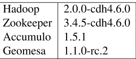
On the other end of the complexity spectrum, by far the most involved and intricate configuration process in preparing for this work was for GeoMesa. It is not a standalone piece of software, but a Java library used by Accumulo, which in turn requires a Hadoop cluster. The three major components used versions shown in Table 2.
Hadoop is the first component to put into place when building what will become the GeoMsea platform. Cloudera’s distribution of Hadoop was used (denoted by the cdh in the version shown in Table 2). This includes core components of Hadoop: Name Nodes, Data Nodes, YARN managers, and Zookeeper nodes. See Section 2.4.1 for details on the functions of each of these components.
be able to access HDFS storage, which Accumulo depends on. With the software deployed and configured, Accumulo processes can be launched and accessed.
Finally, unlike Hadoop and Accumulo, GeoMesa does not have its own java process, but is merely a library for Accumulo to use. Once GeoMesa is built, the JAR file is deployed into
/opt/accumulo/lib/ext, thus adding Geospatial support to Accumulo’s distributed key/value store.
Hadoop 2.0.0-cdh4.6.0 Zookeeper 3.4.5-cdh4.6.0 Accumulo 1.5.1
Geomesa 1.1.0-rc.2
Table 2: Software versions used for cluster infrastructure
Five servers is not a typical size for a production Hadoop system. Usually the benefits of a cluster environment don’t outweigh overhead until a certain scale is reached, often involving many servers. However this provides enough of a cluster to simulate the various roles played by nodes in the cluster: zookeeper nodes, HDFS namenodes (primary/secondary), HDFS datanodes, Accumulo tablet servers, Accumulo monitor node, Accumulo master node, Accumulo tracer node. Some of these overlapped, their distribution is given in Table 3. Since each physical system has 8 CPU cores and 32GB RAM (more detail is shown in Table 5), running multiple services on each is not expected to cause significant performance problems.
For historical reasons, these systems are numbered 03 through 07.
Service Function Server node
03 04 05 06 07
Hadoop
name node X
secondary name node X
data node X X X X X
YARN resource manager X
YARN node manager X X X X X
Zookeeper X X X
Accumulo
Master X
Monitor X
Garbage Collector X
tracer X
slaves X X X X X
Table 3: Service distribution across the available hardware nodes
3.1.3 PostgreSQL/PostGIS server
is not the typical case, so PostgreSQL systems set up that way will fall outside the scope of this work.
This system runs PostgreSQL version 9.3 and PostGIS version 2.1, as provided by Ubuntu version 14.04.
3.2
Building data stores
3.2.1 Generating a Vector Cluster file
The vector cluster file used for testing was provided by collaborators at NRL-SSC, and was built with OpenStreetMap data from planet.openstreetmap.org. Since vector clusters are a write-once read-many format, this process must be manually repeated in order to update the map data with newer information.
After processing theplanet.osmfile, the resulting vector clusterOSM WORLD-0-0-0.vcluster
is 74GB. There are approximately 3 billion objects in OSM dataset.
3.2.2 Ingestion into GeoMesa
In order to make the comparison as unbiased as possible, the identical OpenStreetMap-derived data set was used, by reading through the entireOSM WORLDvector cluster file and inserting each object into GeoMesa.
The NRL layer scheme was preserved, in order to hold that consistent with the Vector Cluster design19. There is a one to one mapping between layers in vcluster to tables in geomesa.
One difference between the way schemas work in GeoMesa and Vector Clusters must be ac-counted for. The Vector Cluster file uses NRL’s feature type (referred to in Java as
mil.navy.nrlssc.commons.vectorData.api.features.Feature<Geometric>,
while GeoMesa uses the Open Geospatial Consortium’s feature type
(org.opengis.feature.Feature). The relevant difference here is that NRL-style features can support variable numbers of attributes, while OGC-style features must have attributes defined in the schema. When working with data from OpenStreetMap, highly variable attributes are a com-mon situation, because of the free-form structure of OSM and due to variations in how millions of users add their (“crowd-sourced”) data.
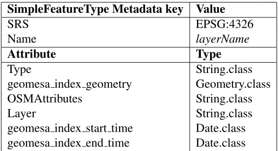
The solution to this disparity is to create an OGC schema with a single OSMAttributes
field, which can be a string of varying length. Then the NRL attributes are concatenated into to a single string, with key/value pairs separated by::: characters. The conversion is simple and only happens during the data insertion, not during the critical path being tested in the next section. (The full SimpleFeatureType schema, including “schema-less” OSMAttributes, is shown in Table 4.)
When looking at storage requirements, due to the way data is replicated in the HDFS storage on which Accumulo and GeoMesa are built, the total disk space required is much higher. This is normal and expected for a distributed, cloud-based cluster system like GeoMesa, and is another (small) part of the higher cost associated.
19However, further testing revealed no significant performance change for individual queries when forgoing layers
SimpleFeatureType Metadata key Value
SRS EPSG:4326
Name layerName
Attribute Type
Type String.class
geomesa index geometry Geometry.class
OSMAttributes String.class
Layer String.class
geomesa index start time Date.class
geomesa index end time Date.class
Table 4: SimpleFeatureType schema used in GeoMesa
3.2.3 Insertion into PostgreSQL
Since the programs to populate the data for both PostGIS and GeoMesa are both written in Java, the schemas (and Java classes) used as our SimpleFeatureTypes are identical. Likewise, one PostGIS layer (and thus one PostgreSQL table) is created for each layer in the Vector Cluster.
The main difference from the GeoMesa insert is that instead of writing a Java object to a “FeatureStore”, the testing software needed to generate SQL statements to insert the data into PostgreSQL. This is easily accomplished using the common JDBC API in Java.
Before inserting the data, it is necessary to create a database in PostgreSQL and then enable PostGIS with the statement:CREATE EXTENSION postgis
In addition to the GiST R-tree index, PostgreSQL provides a module for the hstore data type, which allows for schema-less key-value pairs with support for indexing and querying. This is crucial for storing and searching OpenStreetMap tags in a PostGIS database, as the schemaless key/values map perfectly onto the hstore type. Like PostGIS,hstoreis not built-in to the standard PostgreSQL types, so it must be loaded on each database withCREATE EXTENSION hstore;. However, the tests performed in these experiments were limited to spatial queries, not attribute queries, so while the hstore type was used when inserting OSM data, its features were not userful or relevant to this work.
Once the groundwork is laid by loading the extensions above, the bulk insertion can commence. The Java programInsertFromVectorClusterIntoPostgresmakes a replica of the data stored in theOSM WORLDVector Cluster used in the experiment, by iterating through each feature of the file and writing it to the database with a SQLINSERTstatement.
After all rows of data are inserted, the GiST index is created with: CREATE INDEX [ layer-name idx] ON [layername] USING GIST ( geom );for each feature layer. (While these GIS-style layers are not generally used for OSM’s database, in order to maintain consistency with the Vector Cluster, the same layers/tables will be used here.)
After the insertion and indexing is complete, it is advisable to perform aCLUSTERoperation to optimally reorder the data in the spatial index. However this step was not performed before the measurements described here were made. TheCLUSTERcommand takes considerable time to run on large tables, but it does increase query performance somewhat.
on the database server. This is larger than the the 74GB Vector Cluster, so the various database structures and indices add an overhead of around 7% compared to the simpler flat file.
3.3
Early Experiments
This effort began by working to adapt existing web-based GIS services to utilize a novel storage service, GeoMesa. These services, which provide both raster tiles and vector data, traditionally would use a relational database (for example, PostgreSQL) with geospatial-aware indexing (Post-GIS). The goal was to measure how the same service behaved when the backing storage system changed. In addition to testing against the new and highly complex GeoMesa cluster, a system with nearly opposite design philosophy was also tested: NRL’s Vector Cluster format.
Once a working GeoMesa datastore was built, the first test was to use that datastore for tile serving using OGC’s Geoserver (version 2.5.2), which can be modified to use GeoMesa backend. This was useful to verify the validity of the data store, but Geoserver is a large complex Java application which can be difficult to measure. A simpler visualization of the data was required to proceed.
NRL’s vector server was a better system for testing, with a much simpler interface to the data store. Once this server was adapted to use a GeoMesa backend, it proved stable and useful. Ini-tially, GeoMesa introduced considerable latency and performance cost. But was that cost worth-while above a certain scale?
To address that question, jmeter was used to benchmark under heavy load. The drive was to answer these questions: at what scale does vector cluster “top out”? How much more scalability does a cluster like GeoMesa provide?
Using jmeter and a randomly-generated list of query bounding boxes (using similar methods as those described in Section 3.6), it quickly became clear that vector cluster performance was excellent up to a certain level of load. But when the simultaneous request load went above a certain level20, performance fell off dramatically.
This seemed like a promising result, identifying an inflection point in a curve appeared to be a clear limit of scalability. However, upon further investigation, it turns out that the scalability limit was not in the vector cluster, but in the Tomcat engine handling the HTTP/WMS queries. Another bottleneck came into play before the component of interest was fully utilized.
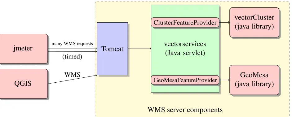
This was an important lesson in testing and measuring complex multi-component services: drawing meaningful conclusions requires focusing narrowly on the specific part of a system, and eliminating other parts of the system as much as possible. Doubtless many researchers have ex-perienced similar lessons with misleading results, but this experience bears repeating, and also informs the subsequent decisions made in this research effort’s experimental design.
Tile servers are intricate collections of software engaged in a complex interaction with net-works, buffers, caches, operating systems, hardware limitations, and much more. Figure 1 shows the parts of the system which testing revealed to influence or interfere with our ability to measure the back-end storage components: GeoMesa and Vector Cluster.
In order to make useful measurements of these systems and find real insights into geospatial data storage practices, it is necessary to eliminate the bottlenecks in other unrelated parts of the
vectorservices (Java servlet) Tomcat
WMS server components jmeter
QGIS
many WMS requests
(timed)
WMS
ClusterFeatureProvider
GeoMesaFeatureProvider
vectorCluster (java library)
GeoMesa (java library)
Figure 1: Early testing apparatus
system. This consideration is what motivated the development of a test harness, described in Section 3.4.
3.4
Refined experimental design
After adapting both NRL’s vector server and Open Source Geospatial Foundation’s Geoserver to use GeoMesa, performance testing began, but it was soon discovered that the bottleneck being measured was not the data back-end, but in the web-front end.
It was then decided to remove all other parts of the tile generation process and focus on isolating and measuring only the query portion, the part of the process where the choice of geospatial storage paradigm is felt.
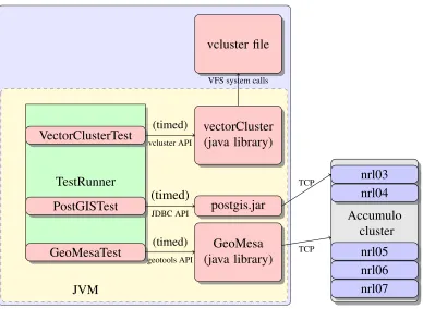
A new testing harness was written in Java, with a TestRunner class, a QueryTest interface, and three classes implementing QueryTest: VectorClusterTest, GeoMesaTest, and PostGISTest. These classes each implement a standardquery()method, such that each can be measured under identical conditions.
Full tile rendering was simulated by querying for all features within a bounding box, for all layers. This results in many queries (turns out to be a bad design decision for a tile service)...
TestRunner
JVM VectorClusterTest
PostGISTest
GeoMesaTest
vectorCluster (java library)
GeoMesa (java library)
(timed)
vcluster API
(timed)
geotools API
vcluster file
VFS system calls
postgis.jar (timed)
JDBC API
cluster Accumulo
TCP
nrl03 nrl04
nrl05 nrl06 nrl07
TCP
Figure 2: Refined testing apparatus
being closer to the real conditions of an active tile server.21
3.5
Measurements
The initialization time for each QueryTest object (GeoMesaTest, VectorClusterTest, or PostGIS-Test) is performed before the stopwatch timer begins. The stopwatch begins when it is time to call thequery()method and stops immediately afterquery()returns.
Each of the three models tested use a form of lazy evaluation for the results returned from queries. After a query is performed, an iterable Collection22is returned but this object may not be fully populated. So in order to truly test the time needed to fetch data from storage, the test harness must iterate through the collection. This effectively “touches” the data, forcing the evaluation of each object in the collection.23
3.6
Simulating tile server workload using randomly chosen bounding boxes
A typical GIS database will contain many layers of vector data. Tile servers generate raster tiles for display by querying the GIS database for vector data, often from many (or all) layers. For a human
21However, without simulated traffic in geographically disparate areas, the test apparatus may gain an unrealistically
high advantage from the page cache. This issue is addressed by the use of the random bounding boxes described in Section 3.6
audience, a layer of data (for example, port facilities) is much more meaningful with context (for example, combining port facilities with coastlines and waterways).
In the dataset used for this experiment, 191 layers have been generated from OpenStreetMap data. As noted earlier, OSM’s database does not use feature layers. But it is not unusual for GIS data consumers to organize data extracted from OSM into GIS layers, as NRL has in their Vector Cluster.
AERIAL
WAY AREAS
Vector
Layer
mor
e layer
s [
. . .
]
WATER
WAY POINTS
Vector
Layer
into:
Raster
map
tile
image
Figure 3: Example of building a tile from queries of many layers
An approximation of the process of generating a raster tile from many vector layers is illustrated in Figure 3.
In order to simulate the workload of a busy map server serving many simultaneous users spread across a large area, a common approach is to scatter requests around a large geographic area. Using an existing tool, simulated map query sample sets (referred to below as “bounding boxes”) were generated for use in testing.
These bounding boxes were generated using wms request.py24, a python program origi-nally written by Frank Warmerdam for the Open Source Geospatial Foundation’s 2009 FOSS4G conference. At that conference, GeoServer, MapServer, and ArcGIS Server competed for the title of “Fastest Web Map Server (WMS)”. [13]
In each test case, one of two sets of 2000 randomly-generated bounding boxes are used. One set of 2000 bounding boxes is across a wide area (described in Section 3.6.1, the other in a smaller, feature-dense region (described in Section 3.6.2).
3.6.1 Within contiguous North America (all-layer tests)
For our tests that generated full-tiles from 191 layers, bounding boxes were used which spread across a contiguous section of North America. The sparseness of features across the area is less of a problem when all layers are queried; empty tiles are less common. This also allows us to simulate more closely a real workload, where queries come in for disparate geographical areas so a server cannot simply cache one region.
Figure 4: Randomly generated bounding boxes across continental North America
3.6.2 Within feature-dense areas (single-layer tests)
In performing tests across North America, it was observed that many randomly generated bounding boxes contained few features, and queries on many layers would yield zero results. Given the vast size and relatively low density of human settlement in North America, it is not surprising that many randomly chosen bounding boxes will end up in a feature-poor region.
The problem of frequent zero-result bounding boxes was addressed by limiting single-layer tests to areas known to be feature-rich. Originally chosen for experiments were: Berlin, Germany, very heavily mapped by OSM volunteers; New Orleans, USA, a much smaller and less dense city; and San Jose, California, roughly somewhere in between the first two cities in terms of size and density. Chosen for presentation in this document are results from the San Jose queries.
Figure 5 shows a visualization of the 500 bounding boxes in and around San Jose, California, used in the single-layer testing. Results from these tests are presented in Sections 4.2.1 and 4.2.2.
3.7
Testing with multithreading (all-layer tests)
The TestRunner class created for this research effort also supports querying all layers within a given bounding box, using a configurable number of simultaneous threads.
Java, as is common for a widely-used, mature language and runtime environment, can be par-allelized using a number of different methods. Some of these include standard components of the JavaTM Platform, such as Timer, ExecutorService, and ForkJoinPool. There are also
third-party libraries such as ParallelJava and Javolution.
Figure 5: Randomly generated bounding boxes in and around San Jose, California
neither the fastest nor the slowest of those tested.[25, pp. 3-19 to 3-22]
3.8
Hardware
To accommodate the experiments described above, a new geospatial computing cluster was built based on these needs. The Vector Cluster and PostGIS systems had simple hardware requirements, but the cluster on which GeoMesa tests would run required new hardware.
In order to create an environment for simulating use of a distributed Hadoop-Accumulo cloud-based GeoMesa service, a multi-node cluster was needed. A relatively small number of servers were acquired, installed, and dedicated to this task.
The experimental cluster consisted of five nodes, each a Dell server with the specifications given in Table 5.
Make and Model DellR
PowerEdge R415
CPU Two 8-core AMDR OpteronTMProcessor 4386 (total 16 CPU cores)
RAM 32GB DDR3 (1600MHz) Synchronous Registered (Buffered)
Disk Toshiba 1TB SATA HDD 7200 RPM
OS kernel Linux 3.13.0 x86 64 OS system Ubuntu 14.04 LTS
Table 5: Experimental hardware
4
Results
Tests from the custom, finely targeted test harness described in Section 3.4 yield data on the three storage systems under consideration, in order to provide observations on how each performs under varying workloads.
4.1
Generalized performance comparison
Before digging into details on how each system behaves under varying conditions, an overall pic-ture of query performance is quite clear. GeoMesa, the distributed-cloud Accumulo-based system, differs greatly from the others in its design, and the resulting behavior of the system is quite dif-ferent.
Vector Cluster and PostGIS are both more traditional designs, and their results lie much closer to one another. All of these are summarized in Table 6, which should be paired with Tables 7 and 8 in the next section when considering overall properties of each paradigm.
System Mean query time (seconds) standard deviation
GeoMesa 17.50 0.6014
Vector Cluster 1.526 0.0552
PostGIS 0.8024 0.0326
Table 6: Overall performance comparison: North America bboxes, full tile (all layers), 7 threads
These figures are extracted from the data based on running queries on all 191 layers (as defined in the original NRL vector cluster file), with 7 simultaneous threads performing queries in parallel. See Section 4.3 for more on the behavior of these systems when the number of threads is varied.
It bears repeating that this measurement is for a specific simulated task: a tile server (such as a WMS server) making queries on many layers in a GIS data store to retrieve vector data, to be used in generating a raster tile. This is a common task, but very different from other GIS tasks.
4.2
Which parameters impact query performance
for each system under different conditions.
By looking at the asymptotic behavior of each system, there is insight to be found in how each system scales, and what sort of tasks that system is suited to.
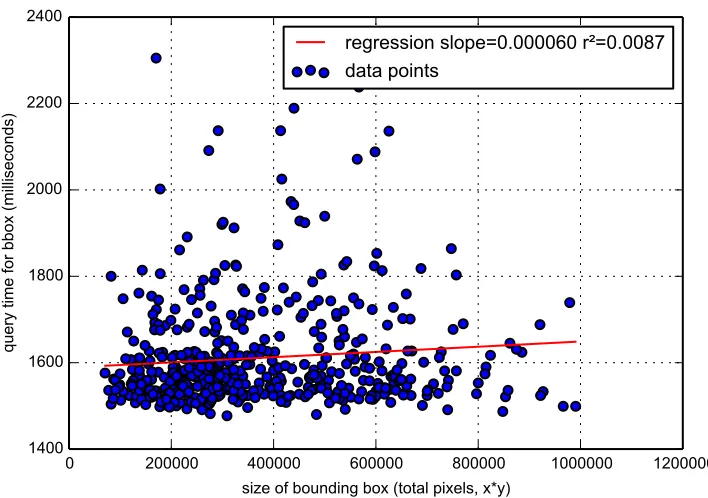
4.2.1 Size of area to be queried
First, for a set of queries over a single feature layer, the size of bounding boxes will be varied, and the impact this change has on query performance is examined.
It may seem intuitive that when searching two regions of the earth for objects (such as building polygons) that intersect these regions, searching the larger region would require more time than searching the smaller one. After all, would you expect “find all buildings in New Orleans” or “find all buildings in Texas” to take longer?
In the thought experiment above, the two regions (New Orleans and Texas) are disjoint and of vastly different size. To generalize this question, also included is the case where the larger region is a superset of the smaller (for example, New Orleans and Louisiana) as well as partially overlapping regions (New Orleans vs. all parts of Louisiana east of the Mississippi River).
It turns out that the intuition about this type of spatial search is wrong. The size of a bounding box does not significantly correlate with the time of a query. This is due to the properties of the R-tree and the fact that the distribution of objects like buildings across the planet is very non-uniform. To continue the thought experiment, it might be considered trivial to find all buildings north of the 85th north parallel (there are none despite the large area) as opposed to finding all buildings in Manhattan (a small place with many buildings).
The very weak correlation between bounding box size and query performance is almost cer-tainly due to the somewhat increased likelihood that a larger bounding box contains more objects to return. As shown in Section 4.2.2, the number of objects returned is a much more important parameter to consider.
In Figure 6, almost no relationship (r2 = 0.0087) is seen between bounding box size and query
performance, when applied to the GeoMesa cluster. This is consistent with what is expected from this type of search: GeoMesa uses a 1-dimensional lexicographically sorted geohash. A bounding box is translated to a set of partitions within the data, represented by prefixes in the key of each row in the Accumulo key-value store. In cases where the data is sparse, fetching all rows with a certain prefix will be fast, regardless of how large that physical area is within the query.
Figure 7 shows the same very weak relationship, with only slightly more effect on PostGIS than in GeoMesa.
And finally in Figure 8 for Vector Cluster, again very low significance. Since Vector Cluster is using an R*tree, it is not surprising to see similar behavior as the R*tree index used in PostGIS. This is also consistent with the understood properties of the R-tree: the depth and complexity of the tree to search is dependent not on physical area, but on the number of leaf nodes (features) within a minimum bouding rectangle (MBR) of arbitrary size.
However, the Vector Cluster data is slightly more significant (r2 = 0.02) than the previous two. In the next section we will explore the way that removing network latency from consideration affects the results for Vector Cluster, the only method we tested that does not involve any network connections.
0 200000 400000 600000 800000 1000000 1200000 size of bounding box (total pixels, x*y)
1400 1600 1800 2000 2200 2400
qu
ery
time
fo
r b
bo
x (mi
llise
co
nd
s)
regression slope=0.000060 r²=0.0087
data points
Figure 6: GeoMesa: query times for varying size bboxes (San Jose highway layer)
0 200000 400000 600000 800000 1000000 1200000
size of bounding box (total pixels, x*y) 0
50 100 150 200 250 300 350
qu
ery
time
fo
r b
bo
x (mi
llise
co
nd
s)
regression slope=0.000023 r²=0.0121
data points
0 200000 400000 600000 800000 1000000 1200000 size of tile (total pixels, x*y)
210 220 230 240 250 260 270 280 290 300
tot
al
qu
ery
time
fo
r ti
le
(mi
llise
co
nd
s)
regression slope=0.000012 r²=0.0264
data points
Figure 8: Vector Cluster: query times for varying size bboxes (San Jose highway layer)
considered CPU-bound. And like many other workloads, CPU-intensive portions of the work are insignificant, in terms of time, compared to other bottlenecks like I/O. This result motivated the next test, given below in Section 4.2.2, where that bottleneck will be examined.
4.2.2 Number of objects returned
Once it is clear that bounding box size is not a significant factor in query performance, the same queries (on the highway layer in San Jose, USA) can be measured on another axis: number of objects returned, or put another way: the payload size.
Figures 9 and 10 show that object count is a far more significant factor in query performance than bounding box size. There are some small differences, however, that are worth noting.
Figure 9 shows a less-tightly-fit regression line (r2 = 0.85) than the data from PostGIS in Figure 10. Essentially the GeoMesa data is noisier. This observation seems consistent with the nature of these systems: GeoMesa is the most complex, built on multiple systems with many sources of latency which can be difficult to measure. PostGIS data in Figure 10 is more tightly fit, as the time to retrieve the data has a very linear relationship with payload size. PostGIS is much simpler, with only one network connection, one hard disk, one virtual memory system, etc, coming into play. So those results are more predicable.
Given the structure of the R-trees, and GeoMesa’s geohash structure, it is not surprising that this query becomes I/O bound rather than CPU bound.
0 500 1000 1500 2000 2500 3000 3500 4000 number of objects returned (query payload size)
1200 1400 1600 1800 2000 2200 2400 2600 2800 3000
qu
ery
time
, si
ng
le
laye
r (mi
llise
co
nd
s)
GeoMesa
regression slope=0.297417 r²=0.8506
data points
Figure 9: GeoMesa: query times for varying object densities (San Jose highway layer)
0 500 1000 1500 2000 2500 3000 3500 4000
number of objects returned (query payload size) 0
100 200 300 400 500 600
qu
ery
time
, si
ng
le
laye
r (mi
llise
co
nd
s)
PostGIS
regression slope=0.118780 r²=0.9261
data points
0 500 1000 1500 2000 2500 3000 3500 4000 number of objects returned
200 220 240 260 280 300 320 340 360 380 qu ery time fo r la ye r (mi llise co nd s)
Vector Cluster
regression slope=0.023185 r²=0.2780
data points
Figure 11: Vector Cluster: query times for varying object densities (San Jose highway layer)
0 500 1000 1500 2000 2500 3000 3500 4000
number of objects returned per query 0 500 1000 1500 2000 2500 3000 qu ery time , si ng le laye r (mi llise co nd s)
All three backends, compared
Geomesa
vCluster
PostGIS
Figure 12: All 3 services, compared
the R*Tree index, and less of the time is spent actually fetching and transferring data, compared to the other two models. As observed above, bounding box size actually was slightly more significant for Vector Cluster than for the others, again confirming that I/O effects like network and disk are much less impactful on this local, flat-file approach.
Finally, Figure 12 shows the previous three results combined, emphasizing the intersection of the vCluster and PostGIS regression lines. This demonstrations the way that the network I/O effects catch up with PostgreSQL when the dataset rises above a certain size.
4.3
Parallelism
As discussed in Section 3.4 and illustrated in Figure 3, a common workload for a tile server would be to generate a raster tile for display to a user by querying a (possibly large) number of layers of vector data. As observed when testing these storage backends as datastores for Geoserver and NRL’s tile server, performing these queries in parallel is essential for any system with query latency (or more simply, any system).
Section 3.7 describes the mechanism used for threading in our test software. The testing ap-proach used was to vary the number of threads used to retrieve the data to build a single tile, in order to find an optimal level of parallelism.
The parallelism tests were conducted over the North America random bounding boxes, shown in Section 3.6.1. For each bounding box, all layers are queried as fast as possible (given the thread concurrency constraint).
In Figures 13, 14 and 15, results are shown for the same workload as the number of threads is increased. The threading levels are colored differently to stand out, and also include a Normal PDF plot.
Like in many other examples of software parallelism, vector cluster performance gains consid-erably when going from 1 to 2 threads, and returns fall off as the number is increased further.
For the Vector Cluster test in Figure 13, 7 threads is the point at which no further improvement can be made by adding more threads. We do see an increase in variability (indicated by a wider, shorter PDF curve) as more threads are added: more threads essentially adds noise.
PostGIS seems to benefit slightly more from multithreaded processing. The test shown in Figure 14 shows the relational database making steady gains up to 8 threads. After 8 threads, very small gains (less than one standard deviation) are made while theσvalue increases: more threads mean more noise and uncertainty. Above 19 threads, the mean time actually gets worse. Between 8 and 19 threads would seem to be ideal; 8 would be preferable, as the benefits of going higher are nearly negligible.
This additional parallelism advantage may be due to PostgreSQL’s long history as a high-performance database system under great concurrency and load.