* Corresponding author. Tel.:+98 912 350 68 63; Fax: +98 21 7322 5098 E-mail: [email protected] (M. MahdaviMazdeh)
© 2013 Growing Science Ltd. All rights reserved. doi: 10.5267/j.ijiec.2012.011.003
Contents lists available at GrowingScience
International Journal of Industrial Engineering Computations
homepage: www.GrowingScience.com/ijiec
A multi supplier lot sizing strategy using dynamic programming
Iman Parsa, Mohsen Emadi Khiav, Mohammad Mahdavi Mazdeh* and Saharnaz Mehrani
Department of Industrial Engineering, Iran University of Science and Technology, Tehran, Iran C H R O N I C L E A B S T R A C T
Article history: Received August 20 2012 Received in revised format November 18 2012
Accepted November 20 2012 Available online
21 November 2012
In this paper, the problem of lot sizing for the case of a single item is considered along with supplier selection in a two-stage supply chain. The suppliers are able to offer quantity discounts, which can be either all-unit or incremental discount policies. A mathematical modeling formulation for the proposed problem is presented and a dynamic programming methodology is provided to solve it. Computational experiments are performed in order to examine the accuracy and the performance of the proposed method in terms of running time. The preliminary results indicate that the proposed algorithm is capable of providing optimal solutions within low computational times, high accuracy solutions.
© 2013 Growing Science Ltd. All rights reserved Keywords:
Supply chain Lot sizing Supplier selection Quantity discounts Dynamic programming
1. Introduction
During the past few years, the significant growth in the industries has resulted in a highly competitive environment where a growing demand for efficiency and effectiveness in companies is observed. Therefore, decision makers have considerably become interested in “supply management” and “inventory management”. The lot sizing problem has a notable influence on inventory and production costs and it has attracted many researchers for over years. The problem is to determine the time and the amount of order or production. It is often difficult to solve the lot sizing problem with supplier selection for the case of multiple suppliers, where each may have a different purchasing, ordering costs, inventory holding costs, etc. Sometimes the suppliers offer quantity discounts, as well. Considering different aspects of the supply chain, discounts can make some improvements. Discounts are supposed to be beneficial for the following reasons:
1. Improving the coordination of the chain
62
The lot sizing problem was first studied by Wagner and Whitin (1958) who provided a dynamic programming algorithm for a problem of multiple periods and a single product. Silver and Meal (1973) proposed a heuristic for solving the problem, called Least Period Cost. Other heuristics were developed by others like Federgruen and Tzur (1991) and Aggarwal and Park (1993). These algorithms were introduced in order to reduce the existing complexity of problems using efficient data structures and control rules, which aim to scale down the search scope. Quantity discounts have been considered (Benton & Whybark 1982) as well as demand uncertainty (Whybark & Williams 1976).
Shaw and Wagelmans (1998) took capacity restrictions into account and Loparic et al. (2001) added sales and safety stocks to the problem. Shortages and startups (Agra & Constantino 1999) and demand time windows (Lee et al. 2001) are among other factors studied in the literature. Babaei et al. (2012) addressed the multi-level lot sizing and scheduling problem for a multi-product flow shop.The supplier selection problem has also been studied in the literature. Ho et al. (2010) and Agarwal et al. (2011) provided a review study for supplier evaluation and selection. The goal of the lot sizing problem for the case of multiple suppliers is to decide which suppliers to order from, along with the lot sizes and the ordering periods (Weberand Current 1993).
In general, the criteria of supplier selection is divided into quantitative (e.g. price) and qualitative (e.g. customer satisfaction) factors. Wind and Robinson (1968) studied the problem when there are conflicting criteria such as compromising between quality and price. A vendor, for example, that sells the products in a lower quality for a lower price. Hassini (2008) took suppliers’ capacities into account and proposed a linear programming model, considering discounts and due dates. A more complicated model was proposed by Liao and Rittscher (2007) adding carrier selection decisions.
Basnet and Leung (2005) solved the supplier selection and lot sizing problem for the case of multiple items using a heuristic method and proposed an integer linear programming formulation. Tempelmeier (2002) solved the problem for the case of a single item with discounts. Moqri et al. (2011) introduced a forward dynamic programming algorithm to solve the single item problem under no discounts assumption.
In this paper, a supply chain consists of two stages, suppliers and a producer, is considered and the lot sizing problem with supplier selection is studied where there are multiple periods and a single item. In addition, two different discount policies are taken into account including all-units and incremental. Then, the modeling formulation of the problem is proposed and it is solved using an algorithm based on dynamic programming. Finally, the performance of this algorithm is examined in terms of running time and accuracy.
This paper is organized as follows: In section 2, the problem is described in details and the assumptions are given. Section 3 consists of the proposed method and the solution procedure is described. A numerical example solved using this algorithm is given in Section 4 and the computational results are proposed in Section 5. At the end, the conclusion of the paper is presented in Section 6.
2. Problem description
Consider a two stage supply chain where a producer buys the raw materials needed, from a variety of suppliers. The problem is to determine the lot sizes as well as the times to make the orders. The assumptions of the problem are as follow,
- The problem is considered for the single item case;
- There is a finite time horizon, which consists of T time periods;
- Shortages are not allowed, and in each period, it is not possible to satisfy demands of earlier periods;
- Inventory holding cost is charged at the end of period stock and it is independent from the
suppliers and changes over time;
- There is no inventory in the beginning and at the end of the planning horizon; - No limitations are considered for the suppliers’ capacities.
- Unit purchasing cost of each period is determined by the suppliers, independently;
- The supplier charges fixed ordering cost each time an order is made. This cost varies over time periods.
- Two discount schemes are taken into account, incremental and all-units. Each supplier is able to provide one of these discount policies.
Parameters and decision variables used in this paper are as follows:
u: Index of suppliers, u =1, 2, 3,K,U t: Index of time periods, t =1, 2, 3,K,T
u
t : Time period in which order is made to supplier u
t
d : Demand for the item in period t
ut
s : Fixed ordering cost of supplier uin period t
ut
Y : Equals 1 if order is made to supplier uin period t, 0 otherwise
t
h : Unit holding cost in period t
t
I : Inventory at the end of period t
ut
X : Amount procured from supplier uin period t
utx
p : Unit purchasing price of supplier uin period twhen the lot size equals x , x =Xut
(
ut)
MC X : Total purchasing cost of Xutitems
ux
n : The discount range of supplier ufor the lot size of x items, nux =1, 2,K,Nu
un
Q : Upper bound of discount range nof supplier u, n=nux andQu0=0 utn
r : Equals 1 if discount range n is selected, 0 otherwise
u
Z : Equals 1 if incremental quantity discount is provided by supplier u, 0 otherwise.
2.1. Mathematical model
Moqri et al. (2011) presented the mathematical model of the problem, when no discounts are considered. The following model allows each supplier to choose its discount policy.
(1)
( )
1 1 1 1 1
min
T U T U T
ut ut ut t t
t u t u t
s Y MC X h I
= = = = =
⎛ ⎞
+⎜ ⎟+
⎝ ⎠
∑∑
∑∑
∑
subject to
(2)
(
)
(
(
( 1))
( 1))
( )
(
(
)
)
(
)
1 1
1 ,
u u
N N
ut u n utx ut u n utn u utx ut utn u
n n
MC X MC Q − P X Q − r Z P X r Z u t
= =
⎛ ⎡ ⎤ ⎞ ⎛ ⎞
=⎜ + ⎣ − ⎦ ⎟ +⎜ ⎟ − ∀
⎝
∑
⎠ ⎝∑
⎠(3)
(
1)
, ,ut un utn
X ≤Q +M −r ∀u t n
(4)
( 1) 1
(
1)
, ,ut u n utn
X ≥Q − + −M −r ∀u t n
(5)
1 1
U
t t ut t
u
I I − X d t
=
64
(6) ,
T
ut ut k
k t
X Y d u t
=
≤
∑
∀(7)
0 1 ,
ut
Y = or ∀u t
(8)
1
1 ,
N
utn n
r u t
=
= ∀
∑
The objective function (1) is used to minimize the total cost, which consists of fixed ordering costs, purchasing costs and holding costs. The first constraint (2) calculates the purchasing cost in different cases according to the discount policy. Eq. (3), Eq. (4) and Eq. (8) determine the discount ranges associated with the amount procured. Eq. (5) is the flow conservation relationship for different periods. Using Eq. (6) and Eq. (7), lot sizes are either equal zero or the cumulative demands of k consecutive periods. The following recursive relation also minimizes the total costs.
(9)
( )
( )
(
( )
)
(
)
(
)
(
)
( )
(
( )
)
(
)
(
)
(
)
(
)
1
1 1
1 1
min min 1 1
min
, min 1 1
t t
j n k u uj u ujx uj
j t u U
n j k n
t u uj u ujx uj
u U
s h d Z MC X Z P X F j
F t
s Z MC X Z P X F t
− ≤ ≤ ≤ ≤ = = +
≤ ≤
⎧ ⎡ ⎛ ⎞⎤⎫
+ + + − + −
⎪ ⎢ ⎜ ⎟⎥⎪
⎪ ⎢ ⎝ ⎠⎥⎪
= ⎨ ⎣ ⎦⎬
⎪ + + − + − ⎪
⎪ ⎪
⎩ ⎭
∑ ∑
(10)
( )
uj(
u n( 1))
ujx uj u n( 1)MC X =MC Q − +P ⎡⎣X −Q − ⎤⎦
Using Eq. (9) and Eq. (10), a dynamic programming methodology is proposed, which reduces the
search space to obtain the solutions from T
U to
(
1)
2T T
U
× +
(Moqri et al. 2011).
3.
The proposed method
In order to solve the problem discussed above, an algorithm based on forward dynamic programming is proposed.
3.1. Solution characteristics
Some of the characteristics of the final solution of the problem for the case of no discounts are presented before the solution procedure.
Lemma1. Procurement from different suppliers in the same period is never optimal, i.e.
(11)
0 ,
st kt
X X = ∀t s≠k
Lemma2. No order is made in periods with inventory.
(12)
( )1 0
st t
X I − =
Proof. (See Basnet & Leung (2005) in the multi item case). ■
Theorem 1
In the optimal solution, each lot size is equal to aggregate demand of the ordering period and k
(13) t k
st i
i t
X d
+
=
=
∑
for a k >0Proof. This theorem is proved using lemma 2. ■
Theorem 2
For each t whereIt =0, periods 1 to t-1 and t to T could be planned independently.
Proof. Wagner and Whitin (1958) proposed this theorem for the single supplier case. Using theorem 1, Moqri et al. (2011) extended this theorem for the case of multiple suppliers. ■
These lemmas and theorems are implemented to gain the optimal solution when discounts are not considered. Otherwise, the proposed algorithm may result in non-optimal solutions, which are proven to be of an acceptable accuracy and obtained within low computational times.
3.2. The solution procedure
The proposed algorithm of this paper first plans the procurement of the demand of the first period. Then, in each stage, the optimal solution of the latest stage is used to find the purchased amount. Here, time periods are supposed to be the programming stages. This recursive relationship helps speed up the procedure by eliminating many of the possible solutions, which are mostly distant from the optimal solution. The algorithm has the following steps.
1. Let t be the period in which the optimal ordering policy is supposed to be determined. Different ordering policies up to this period are determined as well as their costs. The minimum value indicates the best policy at this stage. Note that the policies studied here are the optimal policies of periods 1 to t-1 and different options of ordering in period T.
This procedure is shown in Table 1. Note that the index uindicates that the options consist of purchasing from different suppliers and all of them are taken into account.
Table 1
Tabular calculations in different periods in the proposed algorithm
T ...
3 2
1
{1,2,..,T-1}(T)u
… {1,2}(3)u
{1}(2)u
(1)u 1
… …
({1,2},3)u
(1,2)u 2
… …
…
3
...
…
…
{1,2,…,T} …
{1,2,3} {1,2}
{1}
Optimal option
2. The cost of each option in step 1 is calculated, which consists of holding, fixed ordering and purchasing costs. The holding cost is charged to the end of period stock and is calculated as follows:
(14) 1
T
t t
t
h I
=
∑
In some periods where there is no inventory, fixed ordering cost is charged since ordering has to be made. Purchasing cost is calculated for ordered lots based on the discount scheme provided by the supplier. In the case of incremental quantity discount, Eq. (15) used and Eq. (16) is used otherwise.
(15)
(
)
1 1
T U
ut
t u
MC X
= =
66
(16)
(
)
1 1
T U
utx ut
t u
P X
= =
∑∑
These calculated costs are added to the optimal cost of the earlier periods, and the result is compared with those of other options.
3. If t =T the option with the minimum cost indicates the final solution of the problem and the algorithm is finished. Otherwise, these steps are repeated for t = +t 1.
4.
Numerical Example
In this section, a numerical example is solved using the proposed algorithm. Table 2 and Table 3 represent the data of the given example. Both suppliers provide all-units quantity discounts.
Table 2
General data of the numerical example
s2t
s1t
ht
dt
T
4 4
1 40
1
7 7
2 25
2
4 4
2 30
3
6 5
2 35
4
Table 3
Given prices of the suppliers in the numerical example
2tx
P
( ) 2
2n 1 n
Q − ≤ ≤x Q
1tx
P
( ) 1
1n 1 n
Q − ≤ ≤x Q
4
0≤ ≤x 30
3
0≤ ≤x 40
3
31≤ ≤x 50
2
41≤ ≤x 70
2
51≤x
1
71≤x
The solution procedure is started from the first period. The only option is to procure the demand of the first period from one of the suppliers. The fixed ordering cost of supplier 1 is equal to 4 and the unit purchasing price of 40 items from this supplier is 3 (the first discount range). Therefore, the total cost of buying the demand of the first period from supplier 1 is 4 3 40 124+ × = . The same calculations for supplier 2 result in 4 3 40 124+ × = as well. Due to the fact that both options result in the same cost, each option could be chosen. Now, the second period needs to be investigated.
Different options of this stage consist of the optimal solution of the first stage combined with meeting the demand of the second period. Therefore, the options are: 1) buying the demands of both periods in the first period from supplier 1, 2) buying the demands of both periods in the first period from supplier 2, 3) buying the demand of each period independently from supplier 1 (or period 1 from supplier 2 and period 2 from supplier 1), 4) buying the demand of period 1 from supplier 1 (or 2) and that of period 2 from supplier 2 separately at the beginning of period 2. The cost of each option is calculated and the one with the minimum cost is selected. These options are presented in Table 4.
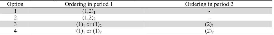
Table 4
Ordering options in period 2 of the numerical example
Option Ordering in period 1 Ordering in period 2
1 (1,2)1 -
2 (1,2)2 -
3 (1)1 or (1)2 (2)1
For periods 3 and 4, the same procedure is applied and different options are compared to find the final solution. These calculations are shown in Table 5 and, as can be seen, the final solution is to procure the demands of periods 1 to 3 from supplier 1 at the beginning of period 1, and buy the demand of period 4 at the beginning of this period from supplier 2. The cost of this ordering policy will be 324.
Table 5
Numerical example calculations
4 3
2 1
(1,2,3,4)1=424
(1,2,3)1=214
(1,2)1=159
(1)1=124 1
(1,2,3,4)2=554
(1,2,3)2=319
(1,2)2=159
(1)2=124 2
(1)1(2,3,4)1 or (1)2(2,3,4)1=414
(1)1(2,3)1 or (1)2(2,3)1=301
(1)1(2)1 or (1)2(2)1=206 3
(1)1(2,3,4)2 or (1)2(2,3,4)2=504
(1)1(2,3)2or (1)2(2,3)2=301
(1)1(2)2 or (1)2(2)2=231 4
(1,2)1(3,4)1 or (1,2)2(3,4)1=363
(1,2)1(3)1 or (1,2)2(3)1=253 5
(1,2)1(3,4)2 or (1,2)2(3,4)2=363
(1,2)1(3)2 or (1,2)2(3)2=283 6
(1,2,3)1(4)1=325 7
(1,2,3)1(4)2=324 8
(1,2,3)1(4)2
(1,2,3)1
(1,2)1 or (1,2)2
(1)1 or (1)2
5. Computational results
In order to evaluate the performance of the proposed algorithm, a computational examination was performed using C++ and Microsoft Visual Studio 2008 on a personal computer (Intel Core2 Quad CPU Q6600 @2.40GHz 2.40 GHz, 2GB RAM). Tables 6, 7 and 8 represent the accuracy of the algorithm in different cases of quantity discounts. The accuracy is indicated by the standard deviation from the optimal solution. In Table 5, the discount policy for all of the suppliers is supposed to be all-units, while in Table 6 it is considered incremental.
In Table 8, discount schemes are chosen by the suppliers independently. As can be seen, three different values are considered for the number of the suppliers as well as the planning horizon. In each case, 10 data sets were randomly generated. The ranges used for the random data are as follows. Demand: (10,40), fixed ordering cost: (10,60), unit holding cost: (1,20) and unit purchasing price: (10,30).
Table 6
Percentage deviations from the exact solution [(Proposed algorithm-Exact)/Exact×100] (All-units)
Num. of Suppliers
Num. of periods
Data set 1
Data set 2
Data set 3
Data set 4
Data set 5
Data set 6
Data set 7
Data set 8
Data set 9
Data
set 10 Mean
3
5 0 0.95 0.83 3.73 0 3.3 19.22 0 5.05 4.16 3.724
10 2.71 12.37 2.32 9.39 16.69 7.14 0.27 3.8 1.1 6.67 6.246
20 2.83 1.03 19.12 0 14.36 14.31 0.24 2.25 4.74 0.73 4.961
4
5 7.99 0 0 6.87 0 5.49 19.8 0 21.93 0.24 6.223
10 7.34 2.75 7.26 5.81 1.32 3 3.29 0.25 4.39 3.08 3.849
20 1.98 2.47 0.94 3.6 16.18 1.37 4.26 0.04 0 23.24 5.408
5
5 0 10.88 0 5.94 17.67 4.93 6.65 2.87 0 0 4.894
10 1.39 3.16 22.61 3.58 0 0 8.74 7.96 18.94 5.94 7.232
20 0.73 24.42 0.84 0 6.34 1.31 16.71 5.65 4.81 6.87 6.768
68
Table 7
Percentage deviations from the exact solution [(Proposed algorithm-Exact)/Exact×100] (Incremental)
Num. of Suppliers
Num. of periods
Data set 1
Data set 2
Data set 3
Data set 4
Data set 5
Data set 6
Data set 7
Data set 8
Data set 9
Data
set 10 Mean
3 10 0 5 0 0.51 3.04 0.670 00 0.181.06 4.390 00 00 1.27 0 0.050 0.1620.955
20 0 0 0.83 0.43 4.33 0 0 0.8 1.36 0 0.775
4 10 0.31 0 1.495 0 0.39 0 0.810 0.720 1.530.24 00 2.750.58 0.34 0 0.480 0.4530.511
20 6.32 0.46 0 0 3.2 0 1.96 0 0 0.44 1.238
5 10 1.43 0 2.335 0.99 0 0 0.540 1.840 0.960 1.150 1.720.4 0 0.810 0 0.4920.725
20 2.17 0.93 0 3.19 1.32 0 0 0 5.17 0 1.278
Table 8
Percentage deviations from the exact solution [(Proposed algorithm-Exact)/Exact×100] (Mixed)
Num. of Suppliers
Num. of periods
Data set 1
Data set 2
Data set 3
Data set 4
Data set 5
Data set 6
Data set 7
Data set 8
Data set 9
Data
set 10 Mean
3
5 0 0.59 0 1.15 0 0 0 0 0.06 0 0.18
10 0 3.07 0.73 0 0.22 4.50 0 0 1.32 0 0.984
20 0 0 0.85 0.43 4.33 0 0 0.8 1.45 0 0.786
4
5 0 0.42 0 0.93 0 0.3 0 2.81 0.39 0 0.485
10 0.32 0 1.56 0 0.78 1.62 0 0.70 0 0.49 0.547
20 6.35 0.49 0 0 3.3 0 2 0 0 0.52 1.266
5
5 1.01 0 0 0.58 1.88 0 1.19 0.46 0 0 0.512
10 1.47 0 2.66 0 0 0.97 0 1.75 0 0.83 0.768
20 2.19 0.97 0 3.29 1.41 0 0 0 5.27 0 1.313
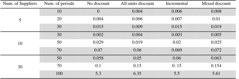
Table 9 represents the running times of the proposed algorithm. Each value in this table represents the average of ten examples that were generated randomly using the following ranges. Demand: (10, 100), unit holding cost: (1, 20), fixed ordering cost: (20, 60) and unit purchasing price: (10, 30).
Table 9
Running times of the proposed algorithm (Seconds)
Num. of Suppliers Num. of periods No discount All-units discount Incremental di
Mixed discount
5
10 0 0.004 0.006 0.008
20 0.004 0.006 0.007 0.01
30 0.015 0.009 0.015 0.019
10
30 0.002 0.004 0.003 0.005
50 0.029 0.019 0.02 0.025
70 0.07 0.06 0.069 0.072
30
50 0.058 0.05 0.06 0.063
70 0.1 0.15 0. 15 0.154
As can be seen, despite large problem sizes, the algorithm solves the problem in low computational times.
6. Conclusion
The problem discussed in this paper is lot sizing along with supplier selection in a supply chain consisted of two stages. The problem is studied in the case of single item, where the demands of different periods are dynamic and known in advance. Suppliers can provide all-units or incremental quantity discounts.
The mathematical model of the problem is presented and an algorithm based on dynamic programming is proposed to solve the problem. The performance of this algorithm has been tested using C++ and Microsoft Visual Studio 2008. The results indicate that the proposed algorithm is able to find high accuracy solutions within low computational times.
References
Agarwal, P., Sahai, M., Mishra, V., Bag, M., & Singh, V.(2011). A review of multi-criteria decision
making techniques for supplier evaluation and selection, International Journal of Industrial
Engineering Computations, 2, 801–810.
Aggarwal, A., & Park, J.K. (1993).Improved algorithms for economic lot-size problems. Operations Research, 41, 549-71.
Agra, A., &Constantino, M. (1999). Lot sizing with backlogging and start-ups: the case of Wagner– Whitin costs. Operation Research Letters, 25, 81-88.
Babaei, M., Mohammadi, M., Fatemi Ghomi, S.M.T., & Sobhanallahi, M.A. (2012). Two parameter-tuned metaheuristic algorithms for the multi-level lot sizing and scheduling problem. International Journal of Industrial Engineering Computations, 3, 751-766.
Basnet, C., & Leung, J.M.Y. (2005). Inventory lot-sizing with supplier selection. Computers and Operations Research, 32, 1–14.
Benton, W.C., &Whybark, D.C. (1982). Material requirements planning (MRP) and purchase discounts. Journal of Operations Management, 2, 137-43.
Federgruen, A., & Tzur, M. (1991). A simple forward algorithm to solve general dynamic lot sizing models with n periods in O(n log n) or O(n) time. Management Science, 37, 909-25.
Hassini, E. (2008). Order lot sizing with multiple capacitated suppliers offering leadtime-dependent capacity reservation and unit price discounts. Production Planning & Control, 19, 142–149.
Ho, W., Xu, X., & K. Dey, P.(2010). Multi-criteria decision making approaches for supplier evaluation and selection: A literature review. European Journal of Operational Research, 202, 1, 16-24.
Liao, Z., & Rittscher, J. (2007). Integration of supplier selection, procurement lot sizing and carrier selection under dynamic demand conditions. International Journal of Production Economics, 107, 502–510.
Loparic, M., Pochet, Y., & Wolsey, L.A. (2001). The uncapacitated lot-sizing problem with sales and safety stocks. Mathematical Programming, 89, 487-504.
Moqri, M., M., MoshrefJavadi, M., &Yazdian, S., A. (2011). Supplier selection and order lot sizing using dynamic programming. International Journal of Industrial Engineering Computations, 2, 319-28.
Shaw, D.X., &Wagelmans, A.P.M. (1998). An algorithm for single-item capacitated economic lot sizing with piecewise linear production costs and general holding costs. Management Science, 44, 831-838.
Silver, E.A., & Meal, H.C. (1973). A heuristic for selecting lot size quantities for the case of a
deterministic time varying rate and discrete opportunities for replenishment. Production and
70
Tempelmeier, H. (2002). A simple heuristic for dynamic order sizing and supplier selection with time-varying data. Production and Operations Management, 11, 499–515.
Wagner, H. M., & Whitin, T.M. (1958). Dynamic version of the economic lot-size model.Management Science, 5, 89-96.
Weber, C., & Current, J. (1993).A multi-objective approach to vendor selection. European Journal of Operational Research, 68, 173-84.
Whybark, D.C., & Williams, J.C. (1976).Material requirements planning under uncertainty. Decision Sciences, 7, 595-606.
![Table 6 Percentage deviations from the exact solution [(Proposed algorithm-Exact)/Exact×100] (All-units)](https://thumb-us.123doks.com/thumbv2/123dok_us/8906018.1834072/7.612.61.543.491.668/table-percentage-deviations-solution-proposed-algorithm-exact-exact.webp)