Static and Dynamic Portfolio Methods for Optimal Planning: An Empirical Analysis

(1)

Static and Dynamic Portfolio Methods for

Optimal Planning: An Empirical Analysis

Mattia Rizzini, Chris Fawcett, Mauro Vallati,

Alfonso E. Gerevini, Holger H. Hoos

Abstract

Combining the complementary strengths of several algorithms through portfolio ap-proaches has been demonstrated to be effective in solving a wide range of AI problems. Notably, portfolio techniques have been prominently applied to suboptimal (satisfic-ing) AI planning.

Here, we consider the construction of sequential planner portfolios for domain-independent optimal planning. Specifically, we introduce four techniques (three of which are dynamic) for per-instance planner schedule generation using problem in-stance features, and investigate the usefulness of a range of static and dynamic tech-niques for combining planners. Our extensive empirical analysis demonstrates the benefits of using static and dynamic sequential portfolios for optimal planning, and provides insights on the most suitable conditions for their fruitful exploitation.

Keywords: automated planning; optimal planning; sequential portfolio; per-instance portfolio generation

1 Introduction

Automated planning is a prominent AI challenge that has been extensively studied for decades and led to a wide range of real-world applications. Within the area of automated planning, cost-optimal (hereinafter, optimal) planning deals with finding optimal plans, i.e., plans that reach a given goal state through an ordered set of actions with minimum total cost. Optimal plans are desirable in many applications.

In recent years, there has been considerable progress in developing powerful domain-independent planners, in no small part spurred on by the International Planning Com-petitions (IPCs)1. However, none of these systems clearly dominates all others in terms of performance over a broad range of planning domains. Furthermore, it has been observed that if a planner does not solve a given problem instance quickly, it will likely not solve it at all within reasonable time[1, 2]. These observations motivate the exploitation of portfolio approaches in planning. In particular, much work has been done in the area of sequential portfolios, where selected algorithms are executed sequentially on a single CPU core. Portfolio approaches, which include algorithm se-lection techniques[3], have been successfully exploited in several other areas, notably satisfiability (SAT) solving and answer set programming (ASP)[4, 5].

1_{http://ipc.icaps-conference.org}

(2)

2 Essential Background on Classical Planning 2

There are planner portfolio configuration systems mainly designed to automatically generate domain-optimized portfolio planners, such as_PbPand _ASAP[6, 7], as well as a range of domain-independent portfolio planners[8]. Among the latter, we can identify two main classes: static portfolios, which run the same schedule of planners on every given problem instance, and portfolios based on per-instance planner schedules.

Cedalion[9] andFast Downward Stone Soup[10] are well-known examples of static portfolio-based planners, while _IBaCoP[11] selects the best planner schedule on a per-instance basis[12]. Here, we introduce a third class, that ofdynamic portfolios, comprised of planners in which the schedule is created dynamically, during execution, based on performance data from earlier runs of the given planners as well as on features of the planning instance to be solved.

Interestingly, we observe that most of the existing work on portfolio-based planners is focused on satisficing planning. However, we note that in IPC-14[13], some static portfolios (MIPlanand DPMPlan), as well as two algorithm selection approaches (NuCeLaRandAllPaca) have participated in the optimal track[12]. These submis-sions were not competitive with the top-ranked planners, but_AllPacaand_NuCeLaR were ranked 7th and 10th respectively. Furthermore, N´u˜nez, Borrajo and Linares[14] mined the results of IPC 2011 by using mixed-integer programming to construct static sequential portfolios of optimal planners; this turned out to be helpful for assessing the usefulness of different sets of training instances, and for better understanding the performance of planners that took part in IPC 2011[15].

In this work, we consider the automatic construction of sequential planner port-folios for domain-independent optimal planning. In particular, we introduce four new techniques: two similarity-based approaches and two model-based approaches. Similarity-based approaches select the algorithms to run by considering performance on training instances deemed sufficiently similar to the given input problem instance. Model-based systems generate a model of the performance of each considered compo-nent planner, which is then exploited for the selection process. Three of our proposed methods are dynamic portfolio approaches.

The sequential portfolios thus obtained are then compared with static planner portfolios and withPlanzilla, an out-of-the-box application of theSATzilla[4, 16] algorithm selection approach to planning. In an extensive empirical analysis we demon-strate the usefulness of portfolio approaches for optimal planning. In particular, we find that (i) our new model-based and similarity-based approaches are more robust in that they generalise better to new domains of planning problems than the static port-folios and_Planzilla; (ii) when the training set is representative of testing problems, our model-based approaches consistently outperform static portfolios. This paper is a continuation of, and expands upon, an earlier version of our work on portfolio selec-tion [17]. Specifically, in this paper we give much more detail on our four new portfolio selection techniques and dynamic portfolio selection in general, present additional ex-perimental results, and discuss our previous results in more detail.

In the remainder of the paper we first give some background on classical planning, describe the portfolio-based optimal planning approaches considered in our work, and then present the design and results of our empirical analysis.

2 Essential Background on Classical Planning

(3)

3 Portfolio-based Optimal Planning 3

state to a desired goal state. Classical planning is a restricted form of AI planning, where the represented environment is static and fully observable, and actions are both deterministic and instantaneous [18].

In a classical planning task, the environmentstatesare defined by sets of grounded predicates, and every grounded predicate holds in a statesif and only if the definition ofscontains it. A planningoperatorois a tuplehname(o),pre(o),eff−(o),eff+(o),cost(o)i where: name(o) = op name(x1, . . . , xk) (op nameis an unique operator name, and

x1, . . . , xkare free variable symbols calledparametersofo);pre(o),eff−(o) andeff+(o) are sets of predicates with variables in{x1, . . . , xk}, that represento’s preconditions, and negative and positive effects, respectively;cost(o) is a numerical value representing o’s cost2_{. Planning}_actions_{are grounded instances of planning operators obtained by} replacing the operator parameters with objects in a given set. An actionaisapplicable in a statesif and only ifpre(a)⊆s. The application ofain a stateswherepre(a)⊆s holds results in state (s\eff−(a))∪eff+(a).

Aplanning domain model is specified by a set of predicates and a set of planning operators. A planning problem instance is specified via a domain model, a set of objects, an initial state and a set of goal predicates. Asolution plan of a planning problem is a sequence of actions such that their consecutive application starting in the initial state results in a state containing all the goal predicates.

Optimal planners are expected to find solution plans that are optimal in terms of their total cost, which is defined as the sum of the costs of the plan actions.

3 Portfolio-based Optimal Planning

In this section, we provide a description of the sequential planner portfolio approaches considered in our investigation – existing approaches from the literature as well as our four new per-instance approaches. Every portfolio approach considered here requires as input a set of planning algorithmsA, a set of training instancesI, and performance measurements for each plannerA∈ Aon eachi∈ I. Here, we measure performance as CPU time required to produce an optimal plan and assign a penalty value if no optimal plan was produced. The penalised average running time (PAR score) is a real number that counts (i) runs that find an optimal plan as the actual running time used and (ii) runs that crash or do not find an optimal plan as ten times the cutoff time (PAR10). PAR scores are commonly used in automated algorithm configuration, algorithm selection and portfolio construction, because using them allows running time to be considered while still placing a strong emphasis on high instance set coverage.

Algorithm 1 outlines the general procedure used by each of our dynamic portfolio selectors, iteratively making the choice of the next component planner and running time cutoff to use based on training data and previous executions. Throughout the text, we use several convenience functions in our pseudocode for brevity:

perf(A,ti,cutoff) returns the scalar performance metric value for component planner Aon training set instanceti when given running time cutoffcutoff;

success(A,ti,cutoff) is an indicator function returning 1 if executing planner A on training set instance ti with running time cutoffcutoff results in an optimal plan, and 0 otherwise;

(4)

Algorithm 1The structure of a generic dynamic schedule selector trained using set of algorithmsAand training instance setI.

input: test instance i, vector of instance features fi, maximum execution timecutoff∈_R+

output: result of running the selector oni

1: function_{abstractDynamicScheduleSelector}(i,fi,cutoff) 2: remaining←cutoff

3: while inot solvedand remaining>0do

4: select current best algorithmA∈ Aand cutoff timet∈R+ 5: r←result of running Aoniwith cutoffmin(t,remaining) 6: remaining←remaining−(running time + overhead time used) 7: end while

8: end function

runtimes(A,instances) returns the set of running times in the training data resulting from executing plannerAon each instance in the setinstances;

concat(v1,v2) returns a new vector that is the concatenation of vectorsv1andv2.

In the remaining subsections, we describe the considered planning instance fea-tures, present the static portfolios andPlanzillaalgorithm selector used for compar-ison, give details on our presolving and backup solving stages, and introduce our two similarity-based and two model-based dynamic portfolio selectors.

3.1 Problem Instance Features

Our per-instance portfolio approaches leverageplanning featuresextracted from each problem instance and domain, a vectorfi of values computed for any given problem instancei. Each feature infiis a numeric value that reflects a specific property of i, such as the average number of out-edges ini’s causal graph, or whetherihas action costs. These features are designed to succinctly describe important aspects of the instance, such that similar instances have similar feature vectors.

In this work, we use the feature set and extraction algorithm introduced by Fawcett et al.[19] This set contains 311 problem instance features, classified into the following seven groups.

PDDL. By considering the PDDL domain and problem files, 49 features are extracted. Features include information about the use and number of object types, the language requirements, the number of operators, etc.

(5)

LPG preprocessing. 6 features are extracted by running the pre-processing phase of

LPG-td[22]. We extract features such as the number of facts, the number

of “significant” instantiated operators and facts, and the number of mutual exclusions between facts.

Torchlight. Torchlight[23] is a tool for analysing local search topology under h+. In this work, it is exploited for extracting 10 features by considering success (sample state proved to not be a local minimum) and dead-end percentages, and statistics over exit distance bounds and preprocessing results.

FD probing. The_LAMA-2011planner[24] is run for 1 CPU second, in order to extract features from the resulting planning trajectory, such as the number of reasonable orders removed, landmark discovery and composition, and the number of graph edges. In total, 16 features belong to this class.

SAT representation. The Madagascar-p planner[25] is used for generating a CNF formula with a planning horizon of 10 time steps. If the creation of the CNF formula is successful, the SATzilla 2012 [16] SAT feature extractor is used for extracting 115 features from 12 classes: problem size features, variable-clause graph features, variable graph features, variable-clause graph features, balance features, as well as features based on proximity to Horn formula, DPLL probing, LP-based, local search probing, clause learning, and survey propagation. The interested reader is referred to Hutter et al.[26] for details on these features.

Success and timing. For each of the aforementioned six extraction procedures, the CPU time required for extraction is recorded, as well as the success (or failure) of the process. The SAT feature extractors additionally report 10 more timing features for extraction time of various subcomponents. In total, 28 features belong to this class.

To the best of our knowledge, this is the most comprehensive set of features available for planning instances.

3.2 Static Portfolios

Static portfolios are those for which the executed schedule of component planner runs is fixed, and does not depend on the input problem instance to be solved. Usually, such portfolios are based solely on the performance of the potential component algorithms on the training instances. Static portfolios are defined by: (i) the subset of component planners that will be run; (ii) the order in which those planners are to be executed; and (iii) the running time allocated to each component planner. Once configured for a given training set, a static portfolio is not adjusted in any way to the problem instances to be solved by it after training is complete.

In this work, we consider two classes of static portfolios. First, in an approach we will simply refer to as “static portfolio” from here on, we used theFast Downward Stone Soup hill-climbing technique[10]. With a target of k planner components

(6)

until no more than k planner components have been added and the time limit has been reached.

For our second static portfolio approach, we use the greedy schedule construction heuristic of Streeter and Smith[27]. This approach starts with an empty portfolio and iteratively adds thehplanner,runtimeipair that maximises the ratio between additional instances solved and running time spent. This can be computed efficiently using only the running times at which a component planner solved a training instance as a potential choice. We will refer to this approach as “Streeter-style”.

3.3 Planzilla

Planzillais an adaptation of the well-known model-based algorithm selection pro-cedure_SATzilla[4, 16] to optimal planning. This and all the following per-instance and dynamic portfolios implement the same general structure, composed of four sepa-rate stages: pre-solving, feature extraction, main and backup solving. The pre-solving stage is essentially a greedily selected static portfolio with a very short running time cutoff (we use theSATzilladefault of 1/90≈1.11% of the total running time bud-get), aimed at solving the easiest problem instances very quickly without expending running time to compute problem instance features. Some problem instances are solv-able within fractions of a second, while complete feature extraction can take minutes for large or difficult instances. If the problem instance is not solved by the pre-solving stage, a model is evaluated that uses a very simple reduced set of instance features to predict whether the full set of features will be computable within the remaining run-ning time. If so, the complete feature set is extracted from the problem instance and

Planzillaproceeds to the main stage. Otherwise,Planzillaswitches to the backup

solving stage. ThePlanzillamain stage makes use of a predictive modelM(fi) (in this case a random-forest-based Empirical Performance Model, or EPM[26, 16]) in or-der to predict the single best component planner to run on a given problem instance i(using the extracted features fi for that instance). Given the selected component plannerA,Planzillauses a separate regression modelregressionA(fi) to predict the

running time required forAto solvei. Planzillawill execute this selected planner for the entirety of the remaining running time. If for any reason execution terminates early without producing an optimal plan,Planzillaswitches to the backup solving stage. This backup solving stage consists of running the single best component plan-ner, as determined by training set PAR10 score, for the remaining available running time.

Our implementation of Planzillauses the default configuration of an early ver-sion of a new, general-purpose Java implementation of _SATzilla called the _*zilla framework, which was generously provided by theSATzilla team. We do not con-sider Planzilla itself to be a contribution of our work presented here. It should also be noted that_Planzillais not, according to our definition, a dynamic portfolio approach.

3.4 Pre- and Backup Solvers

In addition to their use in Planzilla, each of our four per-instance portfolio ap-proaches also makes use of pre-solving and backup solving stages to complement the main portfolio construction stage(s). Pre-solving is performed identically to that of

Planzilla, with 1.11% of the total running time allocated to a greedily-constructed

(7)

training set instances that are solved by the pre-solving stage are removed from the training set used for the main portfolio construction and backup solving stages.

The backup solving stage, however, is not the same as that used byPlanzilla. The_*zilla backup solving mechanism was designed based on the assumption that any failure necessitating the use of the backup solver would come early in any given run (e.g., due to failure to extract features). In the case of planner portfolios this is no longer the case, as a failure can happen during execution of any individual portfolio component. We have therefore extended the backup solving mechanism to also take into account the running time remaining at the time a backup solver is required. This is done by using incremental running time cutoffs (with one minute increment) and determining, for each cutoff time, the component planner with the best PAR10 score on the training set when given that running time cutoff. If the backup solving stage is required during a particular run, we use the component backup planner for the cutoff closest to the remaining running time.

In the following subsections, we describe only the different main stages for each of our new portfolio approaches.

3.5 Similarity-based approaches

Given a previously unseen problem instance to solve, it is reasonable to select a sched-ule containing planners that performed well on training set instances similar to the given input instance. In all four of our approaches, this similarity is determined based on the featuresfiextracted from this instance, with two model-free approaches

(de-scribed in this subsection) and two model-based approaches (de(de-scribed in the next subsection). Our two model-free (or “similarity-based”) approaches are dynamic port-folios and make use of a notion of distance between problem instances in feature space, in this case Euclidean distance after feature normalisation to the interval [0,1]. Boolean features such as PDDL language requirements were assigned 0 or 1, and any categorical instance features were mapped to integer intervals prior to normalization. Normalization was performed using the feature values observed in our training sets, and in cases where subsequent instance feature values exceeded the bounds determined from the training set, values outside the normalized [0,1] bounds were used.

3.5.1 Instance-core-based

(8)

Algorithm 2Instance-core-based schedule selector

input: problem instancei, vector of instance featuresfi, maximum running timecutoff∈_R+_{, distance cutoff}_{distanceCutoff}_∈

R+

1: function_{instanceCoreScheduleSelector}(i,fi,cutoff,distanceCutoff) 2: remaining←cutoff

3: core← {ti∈trainingInstances|distance(ti, i)≤distanceCutoff}

4: while core6=∅andremaining>0 do

5: A←an element ofargmin_A_∈A P

ti∈coreperf(A,ti,remaining)

6: times← {remaining}S

{t∈runtimes(A,core)|t≤remaining}

7: t←minargmax_t_∈_timesP ti∈core

success(A,ti,t)

t

8: r←result of running Aoniwith cutofft

9: if r.status=success then

10: returnr

11: else

12: core←core\ {ti∈core|success(A,ti, t) = 1}

13: remaining←remaining−(r.runtime+ overhead of selection) 14: end if

15: end while

16: end function

3.5.2 Weight-based

This approach does not perform any initial pruning of the training set. Instead, as shown in Algorithm 3, it assigns a weight to each training set instance, equal to the distance between that instance and the input instanceiunder consideration. In each iteration, the performance of every component planner is computed as the weighted sum of the PAR10 scores for that planner on each training instance (using instance weights). The planner with the best performance is selected and, as in the instance-core-based approach, this planner is executed for a running time maximising the ratio of instances solved to running time spent. After each failed run, we once again remove all problem instances from the training set that were solved by the selected planner in the selected running time. If the remaining training instance set becomes empty, the approach proceeds to the backup solving stage.

3.6 Model-based approaches

For our model-based approaches, the choices of the next component planner to run and its running time are made using empirical performance models learned from training data, using the *zilla framework. We implemented a simplified model-based per-instance approach and afull model-based dynamic portfolio.

3.6.1 Simplified model-based

(9)

Algorithm 3Weight-based schedule selector

input: instance i, vector of instance features fi, maximum running time cutoff∈_R+

1: function_{weightBasedScheduleSelector}(i,fi,cutoff) 2: remaining←cutoff

3: inst←trainingInstances

4: while inst6=∅ and remaining>0 do

5: A←an element of argminA∈A

P

ti∈instdistance(i,ti)·perf(A,ti,remaining)

6: times← {remaining}S

{t∈runtimes(A,inst) s.t. t≤remaining}

7: t←minargmax_t_∈_timesP ti∈inst

success(A,ti,t)

t

8: r←result of executingAoniwith cutofft

10: returnr

11: else

12: inst←inst\ {ti∈inst|success(A,ti, t) = 1}

15: end while

16: end function

models. We train a random decision forest classification model M(fi) to perform

algorithm selection (the next planner to run), and a separate regression forest model regressionA(fi) for each planner A that predicts the running time required to find

an optimal plan for the given instancei. After each run of a component planner, that planner is removed as an option from our classification modelM, to prevent a duplicate selection in the next iteration. We run the selected component planner for the predicted running time (or the remaining running time, if that is smaller), until the time budget has been exhausted.

3.6.2 Full model-based

This approach uses the same regression models for component planner running time prediction as for the simplified approach, but the planner selection process is extended by adding a second classification model (using the same learning techniques as the simplified approach) trained on a feature set that has been extended to take previous failed component planner runs into account. The extended feature set adds a Boolean feature and a real-valued feature for each component planner, indicating whether that planner has already been unsuccessfully run on the given problem instance, and for what running time. This second model is used after each failed selected planner run for a given test instance to decide the next planner to run, considering the planners already tried and their running time (the first selected planner is decided using the same “base” classification modelM of the simplified approach described above).

(10)

4 Empirical Analysis 10

Algorithm 4Simplified model-based schedule selector

input: instance i, vector of instance features fi, maximum running time cutoff∈_R+_{, trained model}_M_{, regression models}_regression

A for each com-ponent plannerA∈ A

1: function_{modelBasedScheduleSelector}(i,fi,cutoff, M,regression) 2: remaining←cutoff

3: while remaining>0do

4: A←M(fi)

5: t←min(regressionA(fi),remaining) 6: r←result of running Aoniwith cutofft

8: returnr

9: else

12: end while

13: end function

values for the new features. For each component plannerA∈ Aand instancei∈ Iin the training set, we produce a set offailure running times. These failure running times consist of (i) a short running time ifAcrashes and (ii) the running timetrequired for Ato find an optimal plan fori, plus running times slightly below and abovet, ifAis able to solvei. (Values greater thantare used to take into account randomisation of the planner affectingt.) We then generate the full cross product of component planner combinations (up to a small dimension, given as a parameter of the training process) with their failure running times on iand add the resulting features to the training data. Details for the training of our modified classification model M0 are given in Algorithm 5, where the additional simulated training data is given bysimSchedulesi

for eachi∈ I.

The full model-based approach (outlined in Algorithm 6) allows us to utilise infor-mation from incorrect predictions to inform subsequent planner selections, but due to the greatly-increased size of the training data requires a significantly greater amount of time for training the classification model. In our experiments reported in the fol-lowing, we considered combinations of up to 2 planners chosen from the overall best 5, resulting in an overall training time of 1 CPU week.

4 Empirical Analysis

We report the results from a large-scale empirical study, in which we examined the effectiveness of the described portfolio approaches, as well as the performance of the individual planners used as portfolio components.

4.1 Settings

(11)

DPM-4 Empirical Analysis 11

Algorithm 5Training the model M0

input: set solverPairs ⊆ A2_{, training set} _{trainingInstances} _{⊂ I}_{, set}

sim-Schedules ={simSchedulesi|i∈trainingInstances}

output: trained model

1: function_trainMPrime(solverPairs,trainingInstances,simSchedules) 2: initializeM0

3: for eachA, B∈solverPairs do

4: initializeThA, Bi

5: initializetrainingData⊂ I × A × R

6: for eachi∈trainingInstancesdo

7: for eachschedule∈simSchedulesi do

8: if A∈schedule and B∈schedulethen

9: continue

10: end if

11: left←cutoff−presolvingCutoff−remaining

12: if A∈schedulethen

13: rA←timeout

14: else

15: rA← result of executingA oniwith cutofft

16: end if

17: if B ∈schedulethen

18: rB←timeout

19: else

20: rB← result of executingB oniwith cutofft

21: end if

22: if rA.result 6=success andrB.result6=success then

23: continue

24: else if rA.performance<rB.performance then

25: best←A

26: else

27: best←B

28: end if

29: weight ← value ∈ R, proportional to rA.performance − rB.performance

30: trainingData←trainingDataS_{₍_f

i,best,weight)}

31: end for

32: end for

33: trainThA, BiontrainingData 34: addThA, BitoM0

35: end for

36: returnM0

(12)

Algorithm 6Model-based schedule selector

input: instance i ∈ I, vector of instance features fi, maximum running timecutoff∈R+, trained modelsM andM0

1: function_{modelBasedScheduleSelector}(i,cutoff, M, M0) 2: remaining←cutoff

3: initializestatevector 4: firstRun←true

5: while remaining>0do

6: if firstRun=truethen

7: A←M(fi)

8: firstRun←false

9: else

10: A←M0(concat(fi,state)) 11: end if

12: t←min(regressionA(fi),remaining) 13: r←result of running Aoniwith cutofft 14: if r.status=success then

15: returnr

16: else

17: update statewith resultr

20: end while

(13)

Plan, Dynamic-Gamer,Gamer, Fast Downward Cedalion, hflow,hpp, hpp-ce,Metis,MIPlan,NuCeLaR,RIDA,Rational Lazy A*,SPM&S,SymBA*-1, SymBA*-2. (Detailed descriptions of these planning systems can be found in the IPC-14 systems description[12].) Hereinafter, we will refer to the participants of the competition as “individual planners”, regardless of the approach they exploit for solv-ing plannsolv-ing problems. In our analysis, they are used as basic solver components.

For the sake of readability, in the remainder of our empirical analysis we will use the following terminology:

Model refers to our full model-based approach;

S-Model indicates the simplified version of our model-based approach;

Sim-I and Sim-W refer to the instance-core-based and weight-based similarity ap-proaches, respectively.

StaticX denotes the static portfolio using up toX planners.

Streeter denotes the static portfolio approach of Streeter and Smith [27].

We focused our study on planning domains that have been used in the optimal track of IPC-14:Barman,Cave-Diving,ChildSnack,Citycar,Floortile,GED,Hiking,

Maintenance,Openstacks,Parking,Tetris,Tidybot,TransportandVisitall. For each domain with a randomised problem instance generator, we generated 200 in-stances using the same generator parameter setting distribution as in the IPC.

Instances were divided into training, validation and testing sets. For each domain, the size of the training set was chosen using component planner performance on a sep-arate set of randomly generated instances, such that component planner performance varied by at most 10% of the performance on the entire instance set. These training set sizes were used to partition our separate 200-instance sets for each domain, with thevalidationsets containing 10% (i.e., 20) of the generated instances and thetesting set containing all of the remaining problem instances. This procedure was used in order to select an appropriate training set for each domain, while avoiding component planner runs on testing set instances prior to our experiments. Hereinafter, when we refer to the training, validation and testing sets, we mean the combined sets includ-ing the correspondinclud-ing instances from all of the considered domains. TheGEDdomain unfortunately lacks a random instance generator, so the IPC-14 GEDinstances were included in our testing set only.

All of our experiments were run using nodes of the Compute-Calcul Canada West-Grid Orcinus QDR compute cluster, where each node contains two 2.66 Ghz Intel Xeon X5650 CPUs for a total of 12 cores and 24GB of RAM3. Each of the individual planner runs, as well as runs of our schedule selectors, were limited to a single core and 8GB of RAM. For both training and testing purposes, a cutoff time of 1800 CPU seconds was used, as in the optimal track of IPC-14. In some experiments, we also considered a shorter cutoff time of 300 CPU seconds, for the purposes of examining the efficacy of our approaches when running time is more tightly limited.

In the optimal track of the IPC, planners are usually evaluated by considering only instance set coverage (i.e., number of solved test instances). In our analysis, we evaluate also running time performance by considering the PAR10 score.

(14)

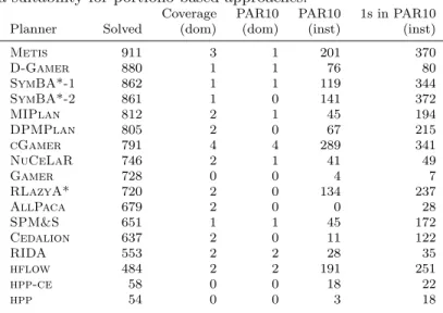
Tab. 1: Individual planner performance on the 2620 testing instances. The total number of solved problems (Solved), the number of planning domains for which that planner had the best coverage (column 3), best PAR10 score (column 4), and the number of problem instances for which that planner either achieved the best PAR10 score (column 5) or was within 1 CPU second of the best PAR10 score (column 6). We note that high performance on individual instances is not limited to the planners with highest instance set coverage, and in fact planners like cGamer andhflowhave very high performance on a large number of instances. This points to an attractive complementarity among these planners, and a suitability for portfolio-based approaches.

Coverage PAR10 PAR10 1s in PAR10 Planner Solved (dom) (dom) (inst) (inst)

Metis 911 3 1 201 370

D-Gamer 880 1 1 76 80

SymBA*-1 862 1 1 119 344

SymBA*-2 861 1 0 141 372

MIPlan 812 2 1 45 194

DPMPlan 805 2 0 67 215

cGamer 791 4 4 289 341

NuCeLaR 746 2 1 41 49

Gamer 728 0 0 4 7

RLazyA* 720 2 0 134 237

AllPaca 679 2 0 0 28

SPM&S 651 1 1 45 172

Cedalion 637 2 0 11 122

RIDA 553 2 2 28 35

hflow 484 2 2 191 251

hpp-ce 58 0 0 18 22

hpp 54 0 0 3 18

4.2 Individual Planners and Static Portfolios

(15)

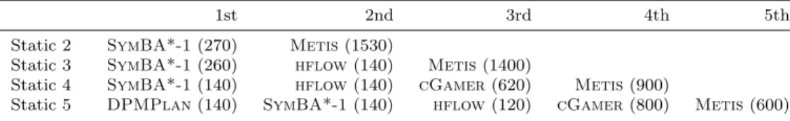
Tab. 2: Basic planners (allocated CPU time) included in the Static portfolios. Planners are listed accordingly to the order in which they are executed.

1st 2nd 3rd 4th 5th

Static 2 SymBA*-1(270) Metis(1530)

Static 3 SymBA*-1(260) hflow(140) Metis(1400)

Static 4 SymBA*-1(140) hflow(140) cGamer(620) Metis(900)

Static 5 DPMPlan(140) SymBA*-1(140) hflow(120) cGamer(800) Metis(600)

which provides the best overall instance set coverage, provides the best PAR10 results in one domain only. In contrast, hflowdoes not provide good overall instance set coverage, but it is the best choice for two of the IPC-14 domains. Similar observations can be obtained on a per-instance basis.Gamershows a peculiar behaviour: it is able to solve a large number of instances, but does not perform particularly well on any domain; it also tends to have high running times on instances it manages to solve. This is due to the approach it exploits: Gamerspends half of the CPU time in creating a heuristic through symbolic search. If a solution is then found, it is immediately re-ported. Otherwise, an abstraction is generated and used for the remainder of the time budget. This suggests that_Gamermay have been specifically configured to perform well for the running time cutoff and scoring function used in the IPC.

Given this promising complementarity between the individual planners under con-sideration, we evaluated the performance of static portfolios combining these planners. We tested portfolios executing 2, 3, 4 and 5 planners, selected via the mechanism out-lined in the previous section. The planners included in the largest static portfolio, ordered according to their allocated CPU time, are: cGamer, Metis, DPMPlan,

SymBA*-1and hflow. Table 2 provides details, in terms of selected planners and

allocated CPU time, of the generated static portfolios.

We also generated a Streeter-style portfolio using the considered basic planners. The generated portfolio includes 7 planners: Metis, SymBA*-1, hflow, RIDA,

DPMPlan,cGamerandSPM&S.

(16)

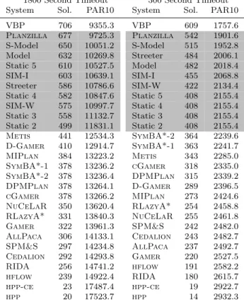
Tab. 3: Number of instances solved and PAR10 scores for the planning sys-tems considered in our study, evaluated with 1800 and 300 CPU second running time cutoffs on our IPC-14 test set. VBP indicates the perfor-mance of the virtual best planner, and grey rows indicate portfolio-based planners. Planners are listed in the order of increasing PAR10.

1800 Second Timeout 300 Second Timeout System Sol. PAR10 System Sol. PAR10

VBP 706 9355.3 VBP 609 1757.6

Planzilla 677 9725.3 Planzilla 542 1901.6

S-Model 650 10051.2 S-Model 515 1952.8 Model 632 10269.8 Streeter 484 2006.1 Static 5 610 10527.5 Model 482 2018.4 SIM-I 603 10639.1 SIM-I 455 2068.8 Streeter 586 10786.6 SIM-W 422 2134.4 Static 4 582 10847.6 Static 5 408 2155.4 SIM-W 575 10997.7 Static 4 408 2155.4 Static 3 558 11132.7 Static 3 408 2155.4 Static 2 499 11831.1 Static 2 408 2155.4

Metis 441 12534.3 SymBA*-2 364 2239.6 D-Gamer 410 12914.7 SymBA*-1 363 2241.7

MIPlan 384 13223.2 Metis 343 2285.0

SymBA*-1 378 13236.2 cGamer 318 2335.0

SymBA*-2 378 13236.4 DPMPlan 315 2339.2

DPMPlan 378 13264.1 D-Gamer 289 2396.5

cGamer 378 13266.2 MIPlan 273 2424.6

NuCeLaR 350 13620.4 RLazyA* 254 2458.8

RLazyA* 331 13840.3 NuCeLaR 255 2461.8

Gamer 322 13961.3 SPM&S 242 2482.0

AllPaca 306 14133.1 Cedalion 243 2482.7

SPM&S 297 14234.8 AllPaca 237 2492.7

Cedalion 292 14293.8 Gamer 220 2527.5

RIDA 256 14741.2 hflow 191 2582.2

hflow 239 14922.4 RIDA 180 2615.7

hpp-ce 23 17487.4 hpp-ce 19 2922.7

hpp 20 17523.7 hpp 14 2932.3

will have insufficient time to increase overall portfolio performance and therefore do not include them.

(17)

4.3 Per-instance Portfolio Performance

In order to evaluate the performance of our four per-instance approaches, as well as that of _Planzilla, we trained each approach using our IPC-14 training set and evaluated the result on the corresponding held-out test set. The running time cutoff for solving each problem instance was 1800 CPU seconds. Instance set coverage and PAR10 scores for each portfolio approach are reported in Table 3, showing that the model-based approaches substantially outperform the static portfolios and similarity-based approaches. In this scenario, the 5-planner static portfolio outperforms the instance-core-based similarity method, and the weight-based similarity method is fur-ther outperformed by the 4-planner static portfolio and the Streeter-style schedule. However, even the similarity-based approaches perform better than all of the individ-ual planners. The fact that the training and test sets were sampled from the same underlying distribution is toPlanzilla’s advantage, as its single planner selection is likely to be correct and the selected planner is able to exploit the large available running time.

To investigate the performance of our per-instance approaches when given a much smaller running time cutoff, we performed another set of experiments with the same training and test sets, but using a 300 CPU second running time cutoff. We observed similar results as for the 1800 CPU second cutoff, but in this case, the similarity-based approaches now outperformed the static portfolios. Interestingly, the Streeter-style schedule performs very well in this case, and its performance was only exceeded by that ofPlanzillaand our simplified model-based approach. We believe that the high performance of the Streeter-style schedule is due to training and test set being drawn from the same distribution, and that by design, this approach performs short runs of many planners. Given a reasonably good selection of planners, and considering the fact that most of the benchmarks can be solved quickly, the observed performance of the Streeter-style approach is not surprising.

4.4 Performance Generalisation to Dissimilar Testing Sets

In order to test the generalisation for all of our considered approaches to planning instances dissimilar from those found in a given training set, we performed two ad-ditional experiments. Because of its high training time (which would have added up to a prohibitive several months of computation on our cluster), we excluded the full model-based approach from this part of our study.

Our first generalisation experiment involved removing all instances from one do-main at a time from our IPC-14 training set, training each approach using this new training set, and then evaluating the result on all problem instances from the held-out domain. We refer to this setup as “leave-one-domain-out”. In Table 4 and Table 5, we present the resulting per-domain instance set coverage using running time cutoffs of 1800 and 300 CPU seconds for solving each instance, respectively.

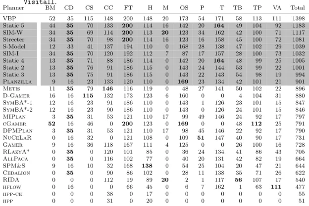
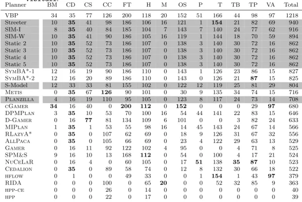
The Streeter-style schedule performed best in this scenario, followed by the two similarity-based approaches and the static portfolios. Our simplified model-based ap-proach and_Planzillaboth fail to generalise as well, and are outperformed by the two

SymBA*planners andMetis, respectively; we believe that this is due to the models becoming overly specialised to the given training set.

(18)

Tab. 4: Number of instances solved per domain by each of the approaches considered in our study, in the “leave-one-domain-out” scenario, using an 1800 second running time cutoff. This allows for a rudimentary analysis of generalisation performance. Results for each of the individ-ual planners have also been included for comparison. Domains, from left: Barman,Cave-Diving,ChildSnack,Citycar,Floortile,Hiking, Maintenance,Openstacks,Parking,Tetris,Tidybot,Transportand Visitall.

Planner BM CD CS CC FT H M OS P T TB TP VA Total

VBP 52 35 115 148 200 148 20 173 54 171 58 113 111 1398 Static 5 44 35 70 133 200 114 16 142 20 164 49 104 92 1183 SIM-W 34 35 69 114 200 113 20 123 34 162 42 100 71 1117 Streeter 34 35 70 98 200 114 16 123 16 158 45 100 72 1081 S-Model 12 33 41 137 194 110 0 168 28 138 47 102 29 1039 SIM-I 34 35 70 120 192 112 7 87 17 157 28 100 73 1032 Static 4 13 35 71 88 186 114 0 142 20 164 48 99 25 1005 Static 2 13 35 76 91 186 115 0 143 24 144 53 99 22 1001 Static 3 13 35 75 91 186 115 0 143 22 143 54 98 19 994

Planzilla 9 16 23 133 120 110 0 169 23 134 42 101 21 901

Metis 11 35 79 146 116 119 0 48 27 141 50 102 22 896

D-Gamer 16 16 115 132 173 123 6 160 0 0 4 104 31 880

SymBA*-1 12 16 23 91 186 110 0 143 1 126 23 101 15 847

SymBA*-2 12 16 23 90 186 110 0 143 0 126 24 101 15 846

MIPlan 3 35 31 53 121 110 17 99 49 146 24 92 17 797

cGamer 52 16 46 0 200 123 0 169 0 0 48 112 25 791

DPMPlan 3 35 31 53 121 110 17 98 45 146 22 92 17 790

NuCeLaR 0 16 32 0 121 108 0 109 51 147 40 90 17 731

Gamer 9 16 36 118 167 111 4 125 0 0 26 100 16 728

RLazyA* 0 35 0 120 101 85 0 36 24 134 41 86 43 705

AllPaca 0 35 0 116 102 77 0 40 20 131 42 82 19 664

SPM&S 9 16 10 32 168 138 0 54 25 104 20 47 21 644

Cedalion 0 35 0 90 86 102 0 28 11 138 35 71 26 622

RIDA 0 0 0 112 19 89 20 2 1 117 56 107 17 540

hflow 0 16 0 0 66 45 0 6 7 162 1 63 111 477

hpp-ce 0 0 0 38 0 17 0 0 0 0 0 0 0 55

hpp 0 0 0 31 0 20 0 0 0 0 0 0 0 51

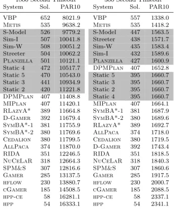
that werenot used in IPC-14. We trained all portfolio-based planners using this new training set and evaluated the result on our IPC-14 test set. This was done with an 1800 CPU second running time cutoff as well as with a 300 CPU second cutoff. The resulting test set coverage and PAR10 scores are summarised in Table 6.

First, we note that the Metisplanner now outperforms all other approaches on the test set. After further investigation, we determined that the_Metisplanner was frequently not the best (or even a good) planner on the domains of our training set, leading to_Metisnot being selected often for problem instances in our test set. This is, of course, a known downside to having a test set that is greatly dissimilar from the instance set used for training.

(19)

Tab. 5: Number of instances solved per domain by each of the approaches considered in our study, in the “leave-one-domain-out” scenario, us-ing a 300 second runnus-ing time cutoff. This allows for a rudimentary analysis of generalisation performance. Results for each of the individ-ual planners have also been included for comparison. Domains, from left: Barman,Cave-Diving,ChildSnack,Citycar,Floortile,Hiking, Maintenance,Openstacks,Parking,Tetris,Tidybot,Transportand Visitall.

Planner BM CD CS CC FT H M OS P T TB TP VA Total

VBP 34 35 77 126 200 118 20 152 51 166 44 98 97 1218 Streeter 10 35 41 98 186 106 16 121 1 154 21 82 69 940 SIM-I 8 35 40 84 185 104 7 143 7 140 24 77 62 916 SIM-W 10 35 41 90 186 105 16 119 1 144 18 70 59 894 Static 2 10 35 52 73 186 107 0 138 3 140 30 72 16 862 Static 3 10 35 52 73 186 107 0 138 3 140 30 72 16 862 Static 4 10 35 52 73 186 107 0 138 3 140 30 72 16 862 Static 5 10 35 52 73 186 107 0 138 3 140 30 72 16 862

SymBA*-1 12 16 19 90 186 110 0 143 1 126 23 86 15 827

SymBA*-2 12 16 20 89 186 110 0 143 0 126 21 87 15 825

S-Model 12 33 33 81 155 102 0 122 12 119 25 81 29 804

Metis 0 35 67 126 90 101 0 30 9 135 34 74 15 716

Planzilla 4 16 19 110 95 105 0 123 8 117 24 73 14 708

cGamer 34 16 40 0 200 112 0 152 0 0 0 29 97 680

DPMPlan 3 35 10 53 70 100 16 54 44 141 22 83 15 646

D-Gamer 0 16 77 81 134 109 6 101 0 0 3 82 24 633

MIPlan 1 35 1 53 55 98 16 14 45 143 24 67 14 566

RLazyA* 0 35 0 107 62 69 0 18 9 126 31 67 32 556

AllPaca 0 35 0 105 66 69 0 23 4 122 29 63 13 529

Gamer 0 16 11 92 122 102 4 95 0 0 4 71 8 525

SPM&S 9 16 10 13 168 112 0 54 0 100 4 17 21 524

NuCeLaR 0 16 4 0 60 105 0 17 51 138 35 87 10 523

Cedalion 0 35 0 89 58 74 0 12 8 132 30 66 18 522

hflow 0 1 0 0 49 33 0 0 1 154 1 43 97 379

RIDA 0 0 0 100 0 65 20 0 0 52 32 85 9 363

hpp-ce 0 0 0 26 0 14 0 0 0 0 0 0 0 40

hpp 0 0 0 22 0 17 0 0 0 0 0 0 0 39

From these generalisation experiments, it appears that different portfolio approaches work best under different circumstances: the model-based approaches are often best in situations where the test instances are likely to be largely similar to those used for training. The similarity-based approaches often perform better when the test set contains many instances from domains not used during training.

4.5 Importance of Pre- and Backup Solvers

(20)

Tab. 6: Number of instances solved and PAR10 scores for the planning systems considered in our study, trained on the IPC 2008 and 2011 benchmarks, evaluated on the IPC 2014 instances. Grey indicates the investigated planner portfolios, while VBP indicates the performance of the virtual best planner. Systems are listed following increasing PAR10 order.

1800 Second Timeout 300 Second Timeout System Sol. PAR10 System Sol. PAR10

VBP 652 8021.9 VBP 557 1338.0

Metis 535 9638.2 Metis 535 1418.2

S-Model 526 9779.2 S-Model 447 1563.5 Sim-I 507 10041.8 Streeter 438 1571.7 Sim-W 508 10051.2 Sim-W 435 1583.4 Streeter 504 10062.2 Sim-I 432 1589.6

Planzilla 501 10121.1 Planzilla 427 1600.9

Static 4 472 10517.7 DPMPlan 407 1652.8 Static 5 470 10543.0 Static 5 395 1660.7 Static 3 441 10934.9 Static 3 395 1660.7 Static 2 420 11221.8 Static 2 395 1660.7

DPMPlan 407 11408.8 Static 4 395 1660.7 MIPlan 407 11420.1 MIPlan 407 1664.1

RLazyA* 389 11664.8 SymBA*-1 381 1687.9

D-Gamer 392 11679.4 SymBA*-2 380 1689.6

SymBA*-1 381 11755.9 RLazyA* 389 1692.7

SymBA*-2 380 11769.6 AllPaca 374 1718.0

Cedalion 380 11799.5 Cedalion 380 1719.5

AllPaca 374 11870.0 D-Gamer 392 1743.4

RIDA 351 12246.5 RIDA 351 1818.5

NuCeLaR 318 12664.3 NuCeLaR 318 1840.3

SPM&S 307 12816.6 SPM&S 307 1860.6

Gamer 285 13137.5 Gamer 285 1917.5

hflow 230 13880.7 hflow 230 2000.7

cGamer 185 14508.5 cGamer 185 2088.5

hpp-ce 58 16281.1 hpp-ce 58 2337.1

hpp 54 16333.1 hpp 54 2341.1

pre-solvers are used as an optimisation for improving the overall running time. Table 7 shows the percentage of problems solved by each stage of our dynamic portfolio approaches; namely presolving, main and backup stages, when using an 1800 CPU second cutoff on our testing set. We observe that the backup solver is rarely exploited, and only the model-based systems use it successfully. This is possibly due to the fact that the backup solver is run only in exceptional cases, such as when feature computation or model evaluation fails. On the other hand, Table 7 clearly shows that pre-solvers are extremely important and responsible for solving a significant percentage of the instances. Given the very limited CPU time available for the pre-solver (1.11% of the cutoff time, around 20 CPU seconds in our experiments), this result is a clear indication that a large number of the benchmarks can be solved in a short amount of time by a single solver. We note that this is especially the case for theFloortile

domain.

(21)

Inter-5 Conclusions 21

Tab. 7: Percentages of instances solved by the pre-solving, main, and backup stages of our four per-instance portfolio approaches, as well as by Planzilla. We also include the percentage of instances left unsolved by each approach.

Pre Main Backup Unsolved

Planzilla 15.0 31.0 0.0 54.0

Model 14.0 28.0 1.0 57.0 SIM-I 20.0 21.0 0.0 59.0 SIM-W 20.0 19.0 0.0 61.0 S-Model 20.0 24.0 1.0 56.0

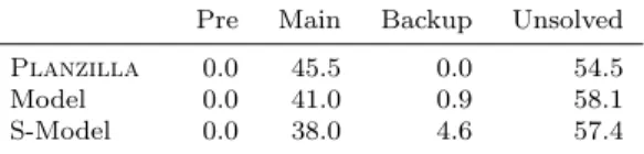
Tab. 8: Percentages of instances solved by model-based approaches and Planzilla, when the pre-solving phase is disabled. We also include the percentage of instances left unsolved by each approach.

Pre Main Backup Unsolved

Planzilla 0.0 45.5 0.0 54.5

Model 0.0 41.0 0.9 58.1 S-Model 0.0 38.0 4.6 57.4

estingly, we observed that the impact on instance set coverage was much smaller than expected. The most affected system is our simplified model-based approach (S-Model), for which disabling pre-solving results in 1.4% fewer instances solved. Apparently, the main solver stage is generally able to solve most of the instances usually solved by the pre-solving stage; we also noticed an increase in the exploitation of backup solvers, which are now used in up to 4.6% of the instances and 10% of the solved instances. This suggests that pre-solving is not fundamental in terms of coverage, but is useful for improving the running time of a portfolio approach. Evaluating the usefulness of the backup solver is straightforward: since it is used only when other steps fail or are believed to be infeasible, its impact can be measured directly as the percentage of instances solved by the backup stage, which was very low in our experiments.

5 Conclusions

In this paper we introduced four new per-instance portfolio techniques, exploiting the largest set of planning instance features currently available [19]. Two of our approaches are model-free and based on similarity metrics in instance feature space. The other two techniques are model-based and iteratively select the next solver to run by con-sidering instance features as well as information about previous failed selections. We compared the performance of these new approaches with that of several static portfolio methods and with the performance ofPlanzilla, an out-of-the-box application of the

SATzillaalgorithm selection system. The results of our extensive empirical analysis showed that:

(22)

5 Conclusions 22

2. if the training instances are representative of testing instances, portfolio-based planners achieve better performance than any individual planner;

3. when training and testing sets include problem instances taken from the same distribution, our new model-based approaches consistently outperform the static portfolios, while our similarity-based approaches match the performance of the static portfolios;

4. when the testing set includes multiple domains not found in the training sets, both our new model-based and similarity-based approaches outperform the static portfolios;

5. our model-based and similarity-based approaches appear to generalise better to previously unseen domains than_Planzilla.

We see several avenues for future work. First, we are interested in further investigating the generalisation performance of the methods considered in our study. In this context, we plan to consider significantly different distributions of problem instances or a larger set of different domains. Secondly, we see promise in studying less expensive but still effective training techniques for variants of our full model-based approach. This might be achievable by selecting more than one planner at a time, thus reducing the number of models to consider in the training step. Thirdly, we are interested in testing the robustness of the portfolio techniques introduced here, with regards to factors such as different hardware and software platforms, or the different configuration of planning domain models. All of these factors have been shown to have remarkable impact on the performance of domain-independent planners [1, 28] and can therefore affect the accuracy of predictive models. We additionally plan to investigate replacing some of our component planners that were themselves portfolio-based with their portfolio components. Finally, we plan to apply our new portfolio approaches to other areas of planning, e.g., temporal or satisficing planning.

Acknowledgements

We thank theSATzillateam (in particular, Chris Cameron) for letting us use a pre-liminary version of their*zilla software. We also gratefully acknowledge computing resources made available by Compute-Calcul Canada. HH and CF were supported by an NSERC Discovery Grant held by HH.

References

[1] A. Howe and E. Dahlman, A critical assessment of benchmark comparison in planning,Journal of Artificial Intelligence Research17(2002) 1–33.

[2] M. Helmert, G. R¨oger and E. Karpas, Fast Downward Stone Soup: A baseline for building planner portfolios, inProceedings of the ICAPS 2011 Workshop on Planning and Learning (ICAPS-PAL)2011, pp. 28–35.

[3] J. R. Rice, The algorithm selection problem,Advances in Computers 15(1976) 65–118.

(23)

5 Conclusions 23

[5] H. Hoos, M. Lindauer and T. Schaub, claspfolio 2: Advances in algorithm selection for answer set programming,Theory and Practice of Logic Programming14(4-5) (2014) 569–585.

[6] A. Gerevini, A. Saetti and M. Vallati, Planning through automatic portfolio con-figuration: The PbP approach, Journal of Artificial Intelligence Research 50

(2014) 639–696.

[7] M. Vallati, L. Chrpa and D. E. Kitchin, ASAP: An Automatic Algorithm Selec-tion Approach for Planning,International Journal on Artificial Intelligence Tools

23(6) (2014).

[8] M. Vallati, L. Chrpa and D. E. Kitchin, Portfolio-based planning: State of the art, common practice and open challenges,AI Communications28(4) (2015) 717–733.

[9] J. Seipp, S. Sievers, M. Helmert and F. Hutter, Automatic configuration of sequen-tial planning portfolios, inProceedings of the Conference on Artificial Intelligence (AAAI)2015, pp. 3364–3370.

[10] J. Seipp, M. Braun, J. Garimort and M. Helmert, Learning portfolios of automat-ically tuned planners, inProceedings of International Conference on Automated Planning and Scheduling (ICAPS)2012, pp. 369–372.

[11] I. Cenamor, T. de la Rosa and F. Fern´andez, The IBaCoP planning system: Instance-based configured portfolios, Journal of Artificial Intelligence Research

56(2016) 657–691.

[12] M. Vallati, L. Chrpa and T. L. McCluskey, The 2014 IPC: Description of Partic-ipating Planners of the Deterministic Track 2014.

[13] M. Vallati, L. Chrpa, M. Grzes, T. L. McCluskey, M. Roberts and S. Sanner, The 2014 international planning competition: Progress and trends,AI Magazine

36(3) (2015) 90–98.

[14] S. Núñez, D. Borrajo and C. L. López, Performance analysis of planning portfo-lios, inProceedings of the Annual Symposium on Combinatorial Search (SOCS) 2012, pp. 65–71.

[15] C. L. L´opez, S. J. Celorrio and ´A. G. Olaya, The deterministic part of the seventh international planning competition,Artificial Intelligence223(2015) 82–119.

[16] L. Xu, F. Hutter, J. Shen, H. H. Hoos and K. Leyton-Brown, SATZilla 2012: Improved Algorithm Selection Based on Cost-sensitive Classification Models, in Proceedings of the SAT Challenge (SC)2012, pp. 57–58.

[17] M. Rizzini, C. Fawcett, M. Vallati, A. E. Gerevini and H. H. Hoos, Portfolio methods for optimal planning: An empirical analysis, inProceedings of the IEEE International Conference on Tools with Artificial Intelligence (ICTAI)2015, pp. 494–501.

[18] M. Ghallab, D. Nau and P. Traverso, Automated planning, theory and practice (Morgan Kaufmann, 2004).

[19] C. Fawcett, M. Vallati, F. Hutter, J. Hoffmann, H. H. Hoos and K. Leyton-Brown, Improved Features for Runtime Prediction of Domain-Independent Planners, in Proceedings of International Conference on Automated Planning and Scheduling (ICAPS)2014, pp. 355–359.

(24)

5 Conclusions 24

[21] I. Cenamor, T. de la Rosa and F. Fern´andez, Mining IPC-2011 results, in Pro-ceedings of the ICAPS 2012 Workshop on the International Planning Competition (ICAPS-IPC)2012.

[22] A. Gerevini, A. Saetti and I. Serina, Planning through stochastic local search and temporal action graphs,Journal of Artificial Intelligence Research20(2003) 239–290.

[23] J. Hoffmann, Analyzing search topology without running any search: On the con-nection between causal graphs and h+,Journal of Artificial Intelligence Research

41(2011) 155–229.

[24] S. Richter and M. Westphal, The LAMA planner: Guiding cost-based anytime planning with landmarks,Journal of Artificial Intelligence Research 39 (2010) 127–177.

[25] J. Rintanen, Engineering efficient planners with SAT, inProceedings of the 20th European Conference on Artificial Intelligence (ECAI)2012, pp. 684–689.

[26] F. Hutter, L. Xu, H. H. Hoos and K. Leyton-Brown, Algorithm runtime predic-tion: Methods & evaluation,Artificial Intelligence206(2014) 79–111.

[27] M. Streeter and S. Smith, New techniques for algorithm portfolio design, in Pro-ceedings of the Conference in Uncertainty in Artificial Intelligence (UAI) 2008, pp. 519–527.