VOLUME 36, ARTICLE 15, PAGES 455
−
500
PUBLISHED 2 FEBRUARY 2017
http://www.demographic-research.org/Volumes/Vol36/15/ DOI: 10.4054/DemRes.2017.36.15
Research Article
Disparities in death: Inequality in cause-specific
infant and child mortality in Stockholm, 1878
‒
1926
Joseph Molitoris
© 2017 Joseph Molitoris.
This open-access work is published under the terms of the Creative Commons Attribution NonCommercial License 2.0 Germany, which permits use, reproduction & distribution in any medium for non-commercial purposes, provided the original author(s) and source are given credit.
1 Introduction 456
2 Background 457
2.1 Maternal factors 459
2.2 Personal illness control 460
2.3 Environmental contamination 461
2.4 Nutrient deficiency 462
3 Data 464
4 Patterns and trends in child mortality in Stockholm 470
5 Multivariate methods 476
6 Event history results 479
7 Discussion 486
8 Acknowledgements 489
References 490
Disparities in death: Inequality in cause-specific infant and child
mortality in Stockholm, 1878‒1926
Joseph Molitoris1
Abstract
BACKGROUND
The decline of child mortality during the late 19th century is one of the most significant demographic changes in human history. However, there is evidence suggesting that the substantial reductions in mortality during the era did little to reduce mortality inequality between socioeconomic groups.
OBJECTIVE
The aim of this study is to examine the development of socioeconomic inequalities in cause-specific infant and child mortality during Stockholm’s demographic transition.
METHODS
Using an individual-level longitudinal population register for Stockholm, Sweden, between 1878 and 1926, I estimate Cox proportional hazards models to study how inequality in cause-specific hazards of dying from six categories of causes varied over time. The categories included are 1) airborne and 2) food and waterborne infectious diseases, 3) other infectious diseases, 4) noninfectious diseases and accidents, 5) perinatal causes, and 6) unspecified causes.
RESULTS
The results show that class differentials in nearly all causes of death converged during the demographic transition. The only exception was the airborne infectious disease category, for which the gap between white-collar and unskilled blue-collar workers widened over time.
CONCLUSIONS
The results demonstrate that, even in a context of falling mortality and a changing epidemiological environment, higher socioeconomic groups were able to maintain a health advantage for their children by reducing their risks of dying from airborne disease to a greater extent than other groups. Potential explanations for these patterns are suggested, as well as suggestions for future research.
CONTRIBUTION
This is the first paper to use individual-level cause-of-death data to study the long-term trends in inequality of cause-specific child mortality during the demographic transition.
1. Introduction
The greatest threats to human health and longevity in historical populations were infectious diseases caused by unsanitary living conditions and unclean food and water, and there was perhaps no group at greater risk of succumbing to these threats than children (see e.g., Mercer 1986; Omran 1971; Preston and Haines 1991). Especially a scourge of industrial cities where transmission was rapid, infectious diseases caused urban mortality rates to dwarf their rural counterparts for much of the industrial era (Cain and Hong 2009; Condran and Crimmins 1980; Knodel 1977). For those children who survived beyond the critical first years of life, the severe disease burden during childhood could have long-lasting impacts on their health and well-being as well as on their individual economic outcomes (Bengtsson and Lindström 2000; Fogel 2004; Hatton 2011; Quaranta 2013). It therefore cannot be overemphasized how important the mortality and health transitions were in improving living standards in both the short and long run, as these changes not only led to greater life expectancy but also a larger share of life spent in good health. Some economists have even argued that such dramatic gains in health and life expectancy may have been important inputs into the transition to modern economic growth (Aksan and Chakraborty 2014; Cervellati and Sunde 2011; Fogel 2004; Fogel and Costa 1997; Morand 2004).
This study aims to shed light on why all-cause mortality inequality persisted by examining how socioeconomic inequality in various causes of death developed during Stockholm’s mortality and health transitions. Although it is beyond the scope of the paper to exactly quantify the influence of various factors (e.g., medical care, sanitation, nutrition) on overall mortality differentials, understanding how the underlying inequalities in cause-specific mortality changed during the period can inform our understanding of the causes behind the process. This is accomplished by using data from an individual-level, longitudinal population register with cause-of-death information to estimate event history models in a competing risks framework. Such an analysis can also provide a multidimensional view of the development of living standards inequality during industrialization. Mortality’s sensitivity to social, economic, and environmental conditions, particularly among children, makes it a strong indicator of living conditions, and as a result it has been incorporated into major standard-of-living indices, such as the Human Development Index (United Nations 1990). The advantage of studying cause-specific rather than all-cause mortality is that different causes of death can be more easily linked to their proximate determinants. This study is unique, as individual-level cause-of-death information is rare in historical settings, especially for a large industrial city like Stockholm. It can therefore also contribute to our understanding of social inequality during the broader urban health transition.
2. Background
The sustained decline of infant and child mortality in Stockholm did not begin until the 1860s (Edvinsson, Garđarsdóttir, and Thorvaldsen 2008). Until then, infant mortality rates were consistently above 300 per 1,000 births, about 20% higher than the rates for Sweden as a whole at the start of its own mortality decline in the late 18th century. Once Stockholm’s mortality rates began to fall, they did so with remarkable speed compared to the experience of the rest of the country. Within 50 years the infant mortality rate in the city had been reduced by more than two-thirds, while the Swedish population needed more than a century to achieve a reduction of the same magnitude.
hazards, such as unclean water and food, and economic growth had led to a threefold increase in the real wages of unskilled workers (Molitoris and Dribe 2016a). It is therefore the aim of this paper to examine how socioeconomic differences in cause-specific infant and child mortality developed in order to better understand how mortality differentials could remain in spite of historical trends, which would seemingly have removed the underlying conditions enabling the perpetuation of inequality in all-cause mortality.
Link and Phelan (1995) provide a framework to explain why, despite large declines in some of the deadliest diseases in the past, socioeconomic differences in health may persist in the long run. They argue that socioeconomic status is a “fundamental social cause” of disease. A fundamental social cause is one which has four main features. First, it influences multiple disease outcomes. Second, those outcomes are affected by more than one risk factor. Third, it involves access to economic and social resources, such as income, knowledge, political clout, and social networks, which can be used to avoid illness as well as to minimize the negative effects of disease. Fourth, the relationship between fundamental causes and health is reproduced over time as new dominant diseases emerge and as knowledge and treatments of disease are developed. It is worth noting that this is not the only framework for understanding socioeconomic differences in mortality over time, as Antonovsky (1967) argues that disparities in mortality follow a pattern of divergence and eventual convergence. This is because the early gains of industrialization first reached higher socioeconomic groups, which led to greater inequality in mortality from nutrition-dependent diseases, but later raised the living standards of the remainder of the population, thereby leading to a convergence of mortality across socioeconomic groups. I have chosen to utilize the ‘fundamental causes’ framework, as it is more explicit about how changes in all-cause mortality differentials relate to changes in the underlying distribution of cause-specific mortality.
related to those sources of exposure. Thus, the degree to which each of the proximate determinants influences overall mortality differentials is not fixed, but rather varies over time as individual resources become more or less important in altering specific sources of exposure.
Although explicitly quantifying the effects of each of the proximate determinants in relation to socioeconomic mortality differentials is beyond the scope of this paper, it is worthwhile to briefly explore how the relative importance of some of these factors may have shifted during Stockholm’s mortality decline, as this will be relevant to interpreting how changes in cause-specific mortality inequality developed during the period.
2.1 Maternal factors
2.2 Personal illness control
Given the state of the medical knowledge of the time, it is also hard to imagine that differences in personal illness control would be responsible for class differences in almost any cause of death, especially prior to the 20th century. Until the late 19th century, smallpox was the only major disease for which an effective therapy existed, and vaccination had already been mandatory for all Swedish children since 1816, suggesting that there should have been no socioeconomic advantage in receiving treatment. Furthermore, smallpox was practically nonexistent in Stockholm after the city’s last serious epidemic in 1874 (Nelson and Rogers 1992). In fact, in the following 25 years of the 19th century there were only 38 registered deaths from smallpox (Stockholm City Research and Statistics Office 2004).
Tuberculosis, on the other hand, was rampant in Stockholm in the late 19th and early 20th centuries (Puranen 1984: 274), especially among children, yet there were no effective treatments for it. At the turn of the 20th century, treatment for tuberculosis consisted of living in sanatoria for months, if not years. There patients were prescribed to breathe fresh air and take walks (Wallstedt and Maeurer 2015). The only way that access to these facilities may have influenced mortality would have been by removing infected individuals from their families, thereby limiting families’ exposure. Considering that these were typically small institutions and that the first state sanatorium was only opened in 1900 (Wallstedt and Maeurer 2015), their influence on mortality inequality most likely was limited.
Of course, personal illness control was not solely related to the use of medical care. Although the importance of advances in general hygienic practices has generally been assigned a secondary role in the mortality decline (McKeown, Brown, and Record 1972), there is evidence that these practices could also have served to reduce mortality in the past and that they may have differed along socioeconomic lines in England and Wales (Razzell 1974). For example, there may have been differences in general cleanliness across groups in terms of washing food or bathing. In Stockholm, it is unclear to what extent these practices varied across groups. Based on schoolchildren’s essays from 1912, well after the start of this study’s coverage, the general view of hygienic living placed a good deal of emphasis on the importance of keeping a home well-lit with sunlight and full of fresh air, and it is easy to imagine how access to these would vary across socioeconomic groups. After all, both of these would be highly contingent on the physical structures in which individuals resided.2 Unfortunately, it is difficult to separate these factors from the role of environmental contamination as a proximate determinant, as many preventative measures, for example, washing food or
bathing, will only be effective illness control strategies if they can be done with clean water.
2.3 Environmental contamination
Differences in environmental exposure to disease were likely much more important for sustaining mortality inequality across socioeconomic groups than differences in maternal factors or medical care. As examples let us consider two common environmental sources of disease in developing contexts: unclean water and residential crowding. The early phases of the expansion of Stockholm’s water network disproportionately favored the wealthier neighborhoods in Stockholm. This is significant, as recent work on the Estonian city of Tartu has shown that educational differences in infant mortality could largely be accounted for by differences in access to clean water (Jaadla and Puur 2016). The city’s first water mains were laid in 1861, primarily near the royal residence and in the well-to-do surrounding areas. Several water pumps were distributed throughout the city and could be used free of charge, but individual property owners were responsible for financing connections to the main network for direct access to the home. This served as an entry barrier to many working-class families and resulted in early declines in child mortality from waterborne diseases among the city’s wealthier inhabitants relative to other socioeconomic groups (Burström et al. 2005). Compounding the problem was the fact that most working-class areas of the city did not have any water mains until several decades after the first pipes were laid (Hansen 1897), meaning that, even if families in these areas could afford to have direct access to clean water, they did not have the possibility of doing so without moving to more expensive districts. By around the turn of the 20th century, piped water had reached most of the population, and this coincided with the equalization of infant and child mortality from some waterborne diseases across socioeconomic groups (Burström et al. 2005), suggesting that individual resources may have become less important in securing clean drinking water than previously.
residential crowding. Figure 1 shows that the share of small apartments in Stockholm’s districts in 1910 had a strong positive correlation with the number of inhabitants per room. Unsurprisingly, districts with a large share of small apartments also tended to have lower rents per room, suggesting that individual resources continued to be extremely important in avoiding exposure to diseases associated with crowding – which also happened to be the deadliest diseases of the day.
Figure 1: Inhabitants per room and rent per room by the share of small apartments in Stockholm’s districts, 1910
Notes: ‘Small apartments’ refers to apartments with one to three rooms and a kitchen.
Source: Stockholm Stads Statistiska Kontor (1912).Statistisk Årsbok för Stockholms Stad 1912 (1910, 1911). Kartogram 2, 3, & 5.
2.4 Nutrient deficiency
much lower proportions of their income on food, but also consumed about 20% more protein per capita (Stockholms Stads Statistiska Kontor 1910). It appears that this discrepancy widened during the first decades of the 20th century. Despite improvements in nutrition for all income groups, a similar survey conducted in 1922 showed that the gap in protein consumption had increased to about 30% (Stockholm Stads Statistiska Kontor 1927), suggesting that nutritional inequality was present in Stockholm well into the 20th century. Figure 2 shows the per capita consumption of low-income households (less than 1,300 kronor) as a share of the per capita consumption of middle-income households (more than 2,000 kronor) as reported in the 1907‒1908 and 1922‒1923 surveys, respectively. What is striking is how the relative differences in consumption widened over only a decade and a half. The growing disparity is especially clear for arguably the most important and relatively inexpensive source of protein for working class families, eggs. In 1907‒1908, higher-income households purchased about 14% more eggs per capita, and this gap had increased to 37% by 1922‒1923. That households with higher levels of income had better nutrition is not surprising, but that this gap increased over time may be an important reason why airborne mortality differentials failed to disappear.
Figure 2: Per capita consumption in low-income households as a share of per capita consumption in middle-income households for specific commodities in 1907‒1908 and 1922‒1923
Notes: Low income refers to individuals with an annual salary less than 1,300 kronor and middle income refers to individuals with a salary of more than 1,950 kronor. These categories were provided by the original surveys. A value of 100% signifies that the per capita consumption of a particular good was equal across income groups in the respective survey, while a value of 50% would indicate that low-income households consumed half the amount of a specific good per capita.
Source:For 1907‒1908: Stockholms Stads Statistiska Kontor (1910). Statistisk Undersökning Angående Lefnadskostnaderna i Stockholm, Åren 1907‒1908. Stockholm: K.L. Beckmans Boktryckeri. For 1922‒1923: Stockholms Stads Statistiska Kontor (1927).
Statistisk Undersökning Angående Levnadskostnaderna i Stockholm 1922/1923. Stockholm: K.L. Beckmans Boktryckeri.
3. Data
city’s borders and to the subdivision of existing districts. To account for this, the 36 districts have been condensed into seven time-invariant districts: Gamla Stan, Norrmalm, Kungsholmen, Östermalm, Södermalm-East, Södermalm-West, and Brännkyrka. At present, data from 26 of the 36 original districts have been digitized. For each individual in the database there is information on birth date and place, location of residence within Stockholm, occupational titles, sex, and position in the household (i.e., servant, lodger, child, etc.). The present work will utilize a subsample of the database that contains individual-level causes of death in addition to the abovementioned information.
Socioeconomic groups were defined by the occupation of the head of household, which could be the mother, father, or, in rare circumstances where the child was adopted by another member of the family, another relative such as an uncle or aunt. Occupations were coded using the Historical International Standard Classification of Occupations (HISCO) (van Leeuwen, Maas, and Miles 2002) and then classified according to HISCLASS (van Leeuwen and Maas 2011), which groups occupations according to the level of skill required, the degree of supervision, and the rural or urban character of work. The original HISCLASS scheme produces 12 distinct categories of workers. However, to avoid problems with small numbers in the multivariate analysis later on, these 12 categories have been condensed into three: 1) white-collar/non-manual workers (HISCLASS 1‒5), 2) skilled manual workers (HISCLASS 6-8), and (3) low-skilled/unskilled manual workers (HISCLASS 9-12). In addition, a fourth category was included for those who had no occupational information available. Among white-collar workers, the majority (about 70%) worked as lower clerical and sales personnel while the remainder had higher management positions or other professions requiring advanced education and experience.
into the digitization of death records was that it was based on district of residence in Stockholm at the time of death (see Appendix Table A-1 for a description of the district selection). In some cases, primary and secondary causes of death are listed, but because this was by no means the norm, this study only utilizes primary cause-of-death information.
It should be noted that historical sources on causes of death are not without problems (see e.g., Risse 1997; Rosenberg 1989). Besides changing definitions of diseases over time, changes in administrative procedures can also affect both the quality and quantity of reporting. Starting in 1749, parish priests in Sweden were required by the Tabular Commission (Tabellverket) to record this information when their parishioners died (Rogers 1999). The difficulty in correctly identifying many causes of death, in addition to the time constraints faced by priests as a result of their wide-ranging responsibilities, could at times lead to under-registration of causes and ambiguous terminology. By the time the present data began (i.e., 1878), the Central Bureau of Statistics (Statistiska centralbyrån) had required for nearly twenty years that urban cause-of-death information be based on death certificates signed by a physician (Rogers 1999). Although this does not ameliorate all problems with the data, it suggests that that information present in the records is as reliable as can be expected for the time. Nevertheless, it is clear from some of the terminology used that doctors were not always able to easily identify the cause of death. There is perhaps no better example for children than the commonly used cause of death, “congenital weakness.”
In a few isolated periods, children in the two blue-collar groups were slightly less likely to have an unreported cause of death than those in the white-collar group, but overall it appears that there was generally no substantial difference in cause-of-death reporting across socioeconomic groups.
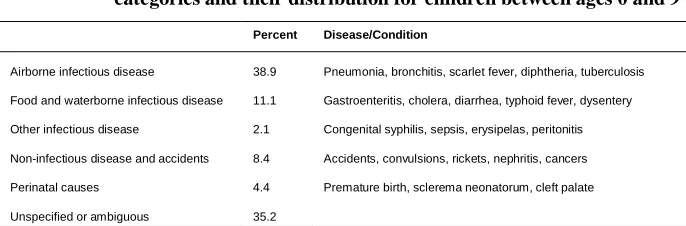
Table 1: Examples of diseases and conditions present in cause-of-death categories and their distribution for children between ages 0 and 9
Percent Disease/Condition
Airborne infectious disease 38.9 Pneumonia, bronchitis, scarlet fever, diphtheria, tuberculosis
Food and waterborne infectious disease 11.1 Gastroenteritis, cholera, diarrhea, typhoid fever, dysentery
Other infectious disease 2.1 Congenital syphilis, sepsis, erysipelas, peritonitis
Non-infectious disease and accidents 8.4 Accidents, convulsions, rickets, nephritis, cancers
Perinatal causes 4.4 Premature birth, sclerema neonatorum, cleft palate
Unspecified or ambiguous 35.2
Notes:Percent column refers to the percentage of dying individuals age 0 to 9.
Source:See Data section.
Although Stockholm’s children were exposed to a vast array of deadly diseases during the late 19th and early 20th centuries, only a handful were responsible for the great majority of deaths. Figure 3 shows the ten most common causes of death among Stockholm’s infants and children between 1878 and 1926. For infants, these ten causes made up about 71% of all deaths with a known cause, while for children they accounted for almost 80%. Infants tended to die from a wider variety of conditions. Deaths from the airborne illnesses of bronchitis and pneumonia alone accounted for just over a quarter of all infant deaths. Diseases of the digestive system were also common killers for infants of the day, evidenced by the high incidence of gastroenteritis, cholera, colitis, and enterocolitis, which together accounted for 23% of all deaths with a known cause. In addition to these, a non-trivial share of infant deaths was attributable to perinatal causes, like birth defects and congenital weakness, which made up about 11% of all deaths.
Figure 3: Ten most common causes of death as a percentage of all deaths with a known cause for infants and children
a) Age 0 to 1
b) Age 1 to 9
Notes:Figures do not include deaths from unknown causes. For infants, the ten most common causes account for 71.4% of all deaths with a known cause (n = 10,515). For children, this figure is 79.3% of all deaths with a known cause (n = 8,547). TB refers to tuberculosis.
4. Patterns and trends in child mortality in Stockholm
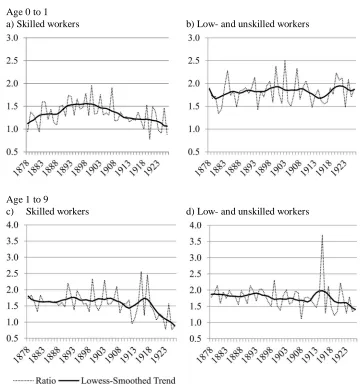
Between 1878 and 1926, the relative difference in age-specific mortality rates between high and low socioeconomic-status groups remained virtually unchanged. Figure 4 shows the development of mortality rates for the age groups 0‒1 and 1‒9 of the two manual worker groups in relation to those experienced by white-collar workers. At the start of observation, under-1 mortality rates for skilled workers’ children were only about 10% higher than for white-collar workers’ children (panel a). As mortality declined, this gap widened until around 1900, when the trend was reversed. By the end of the data’s coverage, the differences between skilled and white-collar workers had begun to converge, and infant children of skilled workers only had about 6% higher rates. This pattern of divergence and convergence was different from that exhibited by lower-skilled groups (panel b). The mortality rates for children below age 1 of low-skilled and unlow-skilled workers were consistently higher than those of white-collar workers.
Figure 4: Age-specific mortality rates relative to white-collar workers by socioeconomic group.
Age 0 to 1
a) Skilled workers b) Low- and unskilled workers
Age 1 to 9
c) Skilled workers d) Low- and unskilled workers
Notes: Figures presented above are the ratios of the corresponding class’s infant mortality in each year to that experienced by the white-collar groups. A locally weighted (LOWESS) regression was used to estimate the smoothed trend using a bandwidth of 0.25 and has been superimposed to clarify the long-term developments of the mortality differentials. LOWESS is a non-parametric approach to smoothing data series that can aid in identifying deterministic trends.
For both infants and children, the period of observation witnessed large declines in overall and cause-specific mortality (Figure 5). The age-specific mortality rate among infants (1m0) was just over 300 per 1,000 person-years lived (PYL) at the start of the
Figure 5: Locally weighted smoothed estimates of infant (age 0 to 1) and child mortality (age 1 to 9) by cause of death
a) Infants (ages 0 to 1)
b) Children (ages 1 to 9)
Notes:Estimates were obtained using a locally weighted regression with a smoothing bandwidth of 0.25 for annual data. Rates are calculated per 1,000 person-years. ‘Overall’ includes all causes of death, including those with unknown causes.
As already alluded to above, the distribution of causes of death among children (ages 1 to 9) was much different from that of infants. Airborne diseases were easily the most dominant cause of death during the entire period, with rates between seven and eight times larger than any other group of causes. Deaths from all other causes were under 2 deaths per 1,000 PYL for nearly the entirety of the period. From this figure it is clear that the decline in child mortality was predominantly due to decreasing airborne disease mortality rates, while for infants the mortality decline was characterized by sequential decreases in different groups of causes. Early on, decreases in food and waterborne mortality and deaths from noninfectious diseases were largely responsible for improvements in infant survival, while later in the decline decreasing mortality from airborne diseases and perinatal causes became relatively more important.
Figure 6: Cause-specific death rates per 1,000 person-years at ages 0‒9 by socioeconomic status
a) Airborne b) Food- and waterborne
c) Other infectious d) Noninfectious and accidents
e) Perinatal causes f) All causes
Notes: Panel e) refers to only age 0–1. Panel f) includes all deaths, including those without a specified cause.
Source: See Data section.
Low and unskilled Skilled workers
5. Multivariate methods
Before implementing an event history analysis it is necessary to accurately identify the population at risk. For this study, individuals who were present at any time in Stockholm between ages 0 and 9 were included in the analysis and censored upon reaching their 10th birthday. This age grouping was taken to avoid problems with small numbers that may arise when including interaction terms in the models. Because causes of death have not been digitized for all districts in Stockholm, only individuals in those districts with recorded causes (i.e., Gamla Stan, Södermalm-East, Södermalm-West) will be considered at risk. As a result, individuals may become at risk only if they were living in any of the included districts between the specified ages. A child would be right censored if he/she moved out of one of these districts before reaching age 10, even if they still resided in Stockholm. However, the child would not be censored if he/she moved from one district with cause-of-death information to another with that information, as district of residence is treated as a time-varying covariate. Individuals could also be left-truncated if they were born outside of the analysis districts and moved into one of them before reaching age 10. Ultimately, the exposure of interest is therefore the number of person-years lived until age 10 in any of Stockholm’s districts with digitized causes of death.
ℎ ( )= ℎ ( )exp( ) (1)
whereℎ ( ) is an individual’s instantaneous risk of dying from causeJ at timet. This is determined by the product of the baseline hazard of dying from cause J (ℎ ) and a vector of covariates, exp(βXi). To estimate this model, separate Cox regressions were
fitted for each cause of death. This means that six models were estimated with the binary dependent variables indicating deaths from: 1) airborne disease, 2) food and waterborne disease, 3) other infectious disease, 4) noninfectious diseases or accidents, 5) perinatal causes, and 6) unknown causes. By using Cox models in a competing risks framework, deaths from causes other than the cause of interest for each regression are treated as a form of censoring. This differs from the commonly used subdistribution hazard model offered by Fine and Gray (1999), which allows individuals dying from competing causes to remain in the risk population (they would remain at risk infinitely for all causes but that from which they died). Both are valid approaches, but have different interpretations. Coefficients in the subdistribution hazard model would be interpreted as the effects of covariates on the cumulative probability of a specific cause of death. On the other hand, in the cause-specific hazard model the coefficients may be interpreted as the influence of the covariates on the instantaneous risk of dying from cause J among those still living and present in the risk population at time t. It has repeatedly been argued that the cause-specific hazard model is more appropriate for studying the etiology of diseases (Lau, Cole, and Gange 2009; Austin, Lee, and Fine 2016), and because this study is specifically interested in the role of socioeconomic status as a fundamental cause of disease, it seems most appropriate to adopt the cause-specific hazards approach for the analysis.
of measuring the other two proximate determinants, nutrient deficiency and personal illness control. To examine how the association between class and causes of death evolved, the models were then extended by including interactions between social class and period dummies. The proportionality assumptions of all models were tested using the method offered by Grambsch and Therneau (1994), which utilizes Schoenfeld residuals. In all models, the main predictor variable, socioeconomic status, showed no signs of nonproportionality. Summary statistics of the covariates may be found in Table 2.
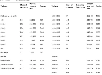
Table 2: Distribution of covariates used in Cox proportional hazards models
Variable Share of
exposure Person years at risk
Deaths Variable Share of exposure
Excluding First-borns
Person years at risk
Deaths
Socioeconomic status: Time since last birth:
White collar 20.9 235,737 3,325 <18 13.1 23.4 147,397 4,480
Skilled workers 26.7 301,725 6,525 18‒23 10.2 18.2 114,540 3,100
Low- and unskilled 46.0 519,022 13,764 24‒29 9.3 16.6 104,836 2,691
Unknown 6.4 71,741 1,802 30‒35 5.7 10.2 64,544 1,667
Birth order 2.4 36‒41 3.6 6.4 40,272 1,072
Female 50.3 567,230 11,858 42‒47 2.6 4.6 29,042 733
Born out of wedlock 10.0 112,683 6,508 48‒53 1.9 3.4 21,534 534
People in household: 54‒59 1.5 2.8 17,409 423
1 to 3 14.4 161,908 5,735 60+ 7.1 12.7 80,004 1,901
4 to 6 45.0 507,559 10,473 Unknown/na 45.1 1.8 508,646 8,815
7 to 9 25.6 289,177 5,888 Period:
Table 2: (Continued)
Variable Share of
exposure Person years at risk
Deaths Variable Share of exposure Excluding First-borns Person years at risk Deaths
Mother's age at birth: 1883‒1887 9.4 105,496 4,117
<20 2.9 33,151 712 1888‒1892 10.2 114,791 3,751
20‒24 19.3 218,285 4,736 1893‒1897 10.7 120,995 3,250
25‒29 28.6 322,636 6,449 1898‒1902 10.3 115,979 3,302
30‒34 24.0 270,627 5,826 1903‒1907 10.4 117,306 2,375
35‒39 15.7 176,902 4,212 1908‒1912 11.3 127,061 2,094
40‒44 6.5 72,912 1,988 1913‒1917 10.9 122,996 1,677
45‒49 1.3 14,574 442 1918‒1922 8.8 98,804 1,055
50+ 1.0 11,753 401 1923‒1926 4.7 53,241 456
Unknown 0.7 7,386 650
District: Season:
Gamla Stan 9.4 106,222 2,354 Spring 20.3 229,299 6,342
Södermalm-East 50.3 567,734 13,592 Summer 24.2 272,948 6,943
Södermalm-West 40.3 454,267 9,470 Autumn 24.8 280,216 5,745
Winter 30.6 345,762 6,386
Notes: Figures for categorical variables refer to the share of total exposure accounted for by the respective category. For birth order, the mean value is presented. ‘Time since Last Birth’ only applies to non-first-born children. All first-borns were assigned an interval of ‘unknown/NA.’ The distribution excluding first-borns is presented to illustrate that very few were missing information on the length of the preceding birth interval.
Source: See Data section.
6. Event history results
blue-collar workers. The differences between groups were the largest for the airborne disease and food and waterborne disease categories. For airborne disease mortality, the children of skilled blue-collar workers were 42% more likely to die than those of white-collar workers, and the gap was even larger among the low- and unskilled blue-collar workers, whose children had a 61% higher risk of dying. The socioeconomic differences regarding mortality from food and waterborne diseases were of a similar magnitude. For most other causes of death the differences between groups were smaller, but still significant in both statistical and real terms. For example, the cause-specific hazards for other infectious diseases were only 26% and 35% higher for the skilled and unskilled groups, respectively, although the estimates for the skilled-workers group was not statistically different from the white-collar group at any conventional significance level. The risk of dying from noninfectious diseases was 25% higher for skilled workers’ children and 28% higher for low- and unskilled workers’ children compared to the white-collar group. There were also differences in dying from perinatal causes, but they were only statistically significant for the children of low- and unskilled workers, who had a 29% higher risk of dying from these causes. That a difference even existed is surprising, as the period of study is one in which prenatal care was virtually absent. It may well be, however, that the existence of a socioeconomic gradient with respect to perinatal causes may reflect differences in maternal nourishment and health.
Table 3: Cause-specific hazard ratios from Cox proportional hazards models
Airborne Food- and water-borne Other infectious Non-infectious Perinatal causes Unknown Socioeconomic status:
White-collar (ref) (ref) (ref) (ref) (ref) (ref) Skilled workers 1.42*** 1.37*** 1.26 1.25*** 1.13 1.23*** Low- and unskilled 1.61*** 1.60*** 1.35*** 1.28*** 1.29*** 1.32***
Unknown 1.06 1.10 1.11 0.83* 1.13 1.26***
Birth order 1.13*** 1.15*** 1.14*** 1.11 1.15*** 1.07***
Female 0.94*** 0.94* 1.14 0.76*** 0.80*** 0.84***
Born out of wedlock 1.93*** 2.83*** 2.73*** 2.12*** 2.82*** 3.35***
People in household:
1 to 3 (ref) (ref) (ref) (ref) (ref) (ref)
Table 3: (Continued)
Airborne Food- and water-borne Other infectious Non-infectious Perinatal causes Unknown
Mother's age at birth:
<20 1.13* 0.86 0.63* 0.85 1.27 0.93
20‒24 (ref) (ref) (ref) (ref) (ref) (ref)
25‒29 0.94* 0.89** 0.84 0.91 0.91 0.88***
30‒34 1.02 0.92 0.82 0.94 0.86 0.82***
35‒39 0.99 0.91 0.77 0.94 1.16 0.87***
40‒44 1.07 0.96 0.82 0.97 1.25* 0.93
45‒49 1.04 1.25 0.59 0.75 0.79 1.00
50+ 0.98 1.55*** 0.42** 0.97 0.62 1.06
Unknown 3.36 3.12*** 2.81*** 3.54*** 3.55*** 2.42*** Time since last birth
(in months):
<18 0.83*** 1.32*** 1.00 1.10 2.01*** 1.08
18‒23 1.06 1.16 1.00 1.08 1.08 1.05
24‒29 1.01 0.93 1.02 0.95 1.03 0.99
30‒35 (ref) (ref) (ref) (ref) (ref) (ref)
36‒41 0.95 0.98 0.98 1.12 1.19 1.20**
42‒47 0.96 0.90 1.12 0.94 1.09 1.10
48‒53 0.85 1.10 1.16 0.95 1.22 1.02
54‒59 0.88 0.91 1.13 0.75 1.09 1.12
60+ 0.75*** 0.96 1.30 0.89 0.99 1.15*
Unknown/na 0.59*** 0.70 0.81 0.81 1.15 0.92
District:
Gamla stan (ref) (ref) (ref) (ref) (ref) (ref)
Södermalm-east 0.72*** 1.39*** 0.94 0.68*** 0.72*** 1.40*** Södermalm-west 0.98 1.33*** 1.20 1.13 0.85 0.68***
Failures 9,883 2,811 538 2,132 1,116 8,936
Individuals 193,833 193,833 193,833 193,833 193,833 193,833 Person-years 1,128,224 1,128,224 1,128,224 1,128,224 1,128,224 1,128,224
Chi2 4,452.9 3,156.3 296.8 954.4 650.6 5,942.9
* Denotes significance at the 10% level, ** Denotes significance at the 5 % level, ***Denotes significance at the 1% level
Notes: A cause-specific hazard ratio of 1.5 indicates that the instantaneous risk of dying from the selected cause is about 50% higher than the reference category. For full model specification and inclusion criteria, see Methods section. Estimates of period and season hazards have been omitted from the output for brevity.
Source:See Data and Methods sections.
for which there was no statistically significant difference between sexes. The difference was most obvious when it came to perinatal causes and noninfectious disease. Girls had a 20% and 24% lower risk of dying from these causes than boys, respectively. Children born out of wedlock had substantially higher risks of dying from all causes relative to those born within marriage, and this association was present independent of socioeconomic and observable maternal characteristics. These children had cause-specific risks of dying that were two to three times as high as those born to married parents. Interestingly, maternal characteristics were very weakly related to most specific causes of death. Children born to mothers who were above age 40 at birth and those born following intervals of less than 18 months had a significantly higher risk of dying from food and waterborne diseases, perhaps due to reduced capacity for breastfeeding. Furthermore, children born following very short intervals also had a much higher risk of dying from perinatal causes, which may be a result of these births being premature (Miller 1989). Otherwise, there were no consistent effects of maternal age or birth spacing on cause-specific hazards.
As for factors related to environmental exposure, there was a strong negative effect of the number of people in the household on all kinds of mortality. This is a surprising finding, as one would suspect that this would have especially facilitated the transmission of infectious disease. It may be, however, that this variable does not capture crowding as much as it captures wealth effects, as wealthier families tended to have larger households via live-in servants. Furthermore, there is no possibility to control for the size of the dwelling, which is equally important to understand the effects of crowding. Some work using the Stockholm Housing Censuses to adjust for the number of inhabitants per m2 has found that the effect of crowding on child mortality was particularly severe among lower socioeconomic groups (Bernhardt 1995). Unfortunately, it is not possible to make this adjustment with the current data. There were also large differences in the risk of dying between districts of the city, though one should not put too much emphasis on the geographic differences as these capture variability in the digitization process as much as they capture differences in the disease environment.
chance of dying from this category of diseases than those of white-collar workers. At the start of observation the difference in risks was only 22%. The gap between low-skilled and unlow-skilled workers’ children and the reference group continuously widened between 1878 and 1926. In the first decade of observation, children from the lowest class were 44% more likely to die from airborne illness than children from the highest class. By 1926 they were more than twice as likely to die from these diseases, and this pattern was quite different from the development of inequality in other causes of death.
Mortality differentials from food and waterborne illness declined in the long run, but only after diverging for several decades. Between 1878 and 1882 the skilled and low- and unskilled blue-collar workers were about 60% and 75% more likely to die from these diseases, respectively. But the gap between the white-collar workers and the other groups widened in the following two decades, reaching its greatest difference at the turn of the 20th century during a period of deadly epidemics. The risk of dying from food and waterborne disease had converged by the second decade of 20th century, first for the children of skilled workers and later for those of low- and unskilled workers. There is some indication that mortality differentials from this group of causes widened again after the First World War, but these estimates were statistically insignificant and based on relatively few cases. These results are consistent with the findings of Burström et al. (2005), who also documented a widening and subsequent closing of diarrheal mortality differentials between socioeconomic groups in Stockholm in the same period. It is also suggestive of class differences in obtaining access to piped water, in which wealthier households were earlier users of sanitation infrastructure than poorer households, likely due to the high costs of connecting buildings to water mains in the earlier years of the water network.
Figure 7: Socioeconomic differences in cause-specific mortality, 1878‒1926
1) Airborne
a) Skilled workers b) Low- and unskilled workers
2) Food- and waterborne
a) Skilled workers b) Low- and unskilled workers
3) Other infectious
Figure 7: (Continued)
4) Noninfectious and accidents
a) Skilled workers b) Low- and unskilled workers
5) Perinatal causes
a) Skilled workers b) Low- and unskilled workers
6) Unknown causes
a) Skilled workers b) Low- and unskilled workers
Notes: Figures presented as hazard ratios. The solid line represents the cause-specific hazard of children of white-collar workers. 95% confidence intervals are reported. All other causes of death are calculated for ages 0 to 9.
Inequality in mortality from noninfectious diseases also disappeared during the study period. There were few statistically significant differences in the risk of dying from this group of causes for the children of skilled workers, though the point estimates indicated an elevated risk of dying for this group. Nevertheless, differences between groups converged by the end of the period. As for the children of low-skilled and unskilled workers, most estimates prior to 1908‒1912 were statistically significant at least at the 10% level and indicated a 20%‒70% higher risk of dying than that experienced by white-collar workers’ children. In the following decades, however, these risks also converged across groups in both statistical and real terms. The convergence observed here was largely due to declining mortality from accidents, seizures, rickets, and nephritis.
Finally, class differences in mortality from perinatal causes were generally non-existent. The only exception to this was in the period 1903‒1907, which saw particularly deadly outbreaks of many infectious diseases, including measles, scarlet fever, pertussis, diphtheria, and tuberculosis, and which may have indirectly affected the incidence of perinatal causes via changes in maternal health. However, apart from short-term differences, inequalities in death from congenital causes were largely absent. The point estimates for low-skilled and unskilled workers’ children seem to be trending towards greater inequality towards the end of the period, although the estimates remained statistically insignificant at any conventional level.
7. Discussion
This paper has demonstrated how socioeconomic cause-specific mortality differentials evolved during Stockholm’s mortality transition, and how these differences contributed to inequality in all-cause child mortality. Prior to 1900, class differences in all-cause mortality were due to a combination of differential mortality rates from airborne, food and waterborne, and, to a lesser degree, noninfectious diseases. However, from the end of the first decade of the 20th century, socioeconomic mortality differentials were almost entirely driven by differences in airborne disease mortality, apart from episodic divergences in mortality risks from other causes. For all other causes of death, mortality inequality had either disappeared by this point or, in the case of perinatal causes, had not been present to begin with.
late 19th century. At the same time the results show that other causes of death became even more unequally distributed. In the case of Stockholm, it was the much more common and lethal airborne infectious diseases such as diphtheria, measles, pneumonia and tuberculosis that filled this niche. Hazards of other causes for which etiology was unclear, such as those associated with premature births and congenital conditions, were statistically indistinct across socioeconomic groups over time. All of these findings are consistent with the theory of fundamental causes (Link and Phelan 1995): Conditions which were poorly understood were not stratified by socioeconomic status, while those for which personal resources became less important for avoiding exposure to proximate determinants became less so over time.
However, the question remains of in what ways the greater resources of higher-status individuals reduce their children’s exposure to airborne diseases and allow them to maintain a health advantage. Unfortunately, the analyses in this study were only able to account for some of the proximate determinants of mortality and therefore cannot identify precisely the influence of various health inputs. However, based on the discussion in Section 2 and the findings from the event history models, some broad conclusions can be made to guide future research in answering this question.
8. Acknowledgements
References
Aksan, A.M. and Chakraborty, S. (2014). Mortality versus morbidity in the demographic transition. European Economic Review 70(1): 470‒492. doi:10.1016/j.euroecorev.2014.06.011.
Antonovsky, A. (1967). Social class, life expectancy and overall mortality. Milbank Quarterly45(2): 31‒73.doi:10.2307/3348839.
Antonovsky, A. and Bernstein, J. (1977). Social class and infant mortality. Social Science and Medicine 11(8): 453‒470.doi:10.1016/0037-7856(77)90022-1.
Austin, P.C., Lee, D.S., and Fine, J.P. (2016). Introduction to the analysis of survival data in the presence of competing risks. Circulation 133(6): 601‒609. doi:10.1161/CIRCULATIONAHA.115.017719.
Bengtsson, T. (2004). Mortality and social class in four Scanian parishes, 1766‒1865. In: Bengtsson, T., Campbell, C., and Lee, J.Z. (eds.). Life under pressure: Mortality and living standards in Europe and Asia, 1700‒1900. Cambridge: MIT Press: 135‒172.
Bengtsson, T. and Lindström, M. (2000). Childhood misery and disease in later life: The effects on mortality in old age of hazards experienced in early life, southern Sweden, 1760‒1894. Population Studies 54(3): 263‒277. doi:10.1080/7137 79096.
Bernhardt, E. (1995). Crowding and child survival in Stockholm 1895‒1920. In Lundh, C. (ed.).Demography, economy and welfare. Lund: Lund University Press: 279‒ 291.
Breschi, M., Fornasin, A., Manfredini, M., Mazzoni, S., and Pozzi, L. (2011). Socioeconomic conditions, health and mortality from birth to adulthood, Alghero 1866–1925. Explorations in Economic History 48(3): 366‒375. doi:10.1016/j.eeh.2011.05.006.
Burström, B. and Bernhardt, E. (2001). Social differentials in the decline of child mortality in nineteenth century Stockholm. European Journal of Public Health 11(1): 29‒34.doi:10.1093/eurpub/11.1.29.
Cain, L. and Hong, S.C. (2009). Survival in 19th century cities: The larger the city, the smaller your chances. Explorations in Economic History 46(4): 450‒463. doi:10.1016/j.eeh.2009.05.001.
Cervellati, M. and Sunde, U. (2011). Life expectancy and economic growth: The role of the demographic transition. Journal of Economic Growth 16(2): 99‒133. doi:10.1007/s10887-011-9065-2.
Conde-Agudelo, A., Rosas-Bermudez, A., Castaño, F., and Norton, M.H. (2012). Effects of birth spacing on maternal, perinatal, infant, and child health: A systematic review of causal mechanisms.Studies in Family Planning43(2): 93‒ 114.doi:10.1111/j.1728-4465.2012.00308.x.
Condran, G. and Crimmins, E. (1980). Mortality differentials between rural and urban areas of states in the northeastern United States 1890‒1900. Journal of Historical Geography6(2): 179‒202.doi:10.1016/0305-7488(80)90111-5.
Edvinsson, S., Brändström, A., Rogers, J., and Broström, G. (2005). High-risk families: The unequal distribution of infant mortality in nineteenth-century Sweden. Population Studies59(3): 321‒337.doi:10.1080/00324720500223344.
Edvinsson, S., Garđarsdóttir, Ó., and Thorvaldsen, G. (2008). Infant mortality in the Nordic countries, 1780–1930. Continuity and Change 23(3): 457‒485. doi:10.1017/S0268416008006917.
Fine, J.P. and Gray, R.J. (1999). A proportional hazards model for the subdistribution of a competing risk. Journal of the American Statistical Association 94(446): 496‒509.doi:10.1080/01621459.1999.10474144.
Fogel, R.W. (2004). The escape from hunger and premature death, 1700‒2100.New York: Cambridge University Press.doi:10.1017/CBO9780511817649.
Fogel, R.W. and Costa, D.L. (1997). A theory of technophysio evolution, with some implications for forecasting population, health care costs, and pension costs. Demography34(1): 49‒66.doi:10.2307/2061659.
Geschwind, A. and Fogelvik, S. (2000). The Stockholm Historical Database. In Hall, P.K., McCaa, R., and Thorvaldsen, G. (eds.). Handbook of international historical microdata for population research. Minneapolis: Minnesota Population Center: 207‒231.
Haines, M.R. (1989). Social class differentials during fertility decline: England and Wales revisited. Population Studies43(2): 305‒323. doi:10.1080/00324720310 00144136.
Haines, M.R. (2011). Inequality and infant and childhood mortality in the United States in the twentieth century. Explorations in Economic History 48(3): 418‒428. doi:10.1016/j.eeh.2011.05.009.
Hansen, F.V. (1897). Stockholms vattenledning. In Dahlgren, E.W. (ed). Stockholm: Sveriges hufvudstad skildrad med anledning af allmänna konst- och industriutställningen 1897. Stockholm: K.L. Beckmans boktryckeri.
Hatton, T.J. (2011). Infant mortality and the health of survivors: Britain, 1910‒50. Economic History Review 64(3): 951‒972. doi:10.1111/j.1468-0289.2010. 00572.x.
Hobcraft, J.N., McDonald, J.W., and Rutstein, S.O. (1983). Child-spacing effects on infant and early child mortality. Population Index49(4): 585‒618.doi:10.2307/ 2737284.
Hobcraft, J.N., McDonald, J.W., and Rutstein, S.O. (1985). Demographic determinants of infant and early child mortality: A comparative analysis.Population Studies 39(3): 363‒385.doi:10.1080/0032472031000141576.
Jaadla, H. and Puur, A. (2016). The impact of water supply and sanitation on infant mortality: Individual-level evidence from Tartu, Estonia, 1897‒1900.Population Studies 70(2): 163‒179.doi:10.1080/00324728.2016.1176237.
Knodel, J. (1977). Town and country in nineteenth-century Germany: A review of urban-rural differentials in demographic behavior. Social Science History1(3): 356‒382.doi:10.1017/S0145553200022112.
Lau, B., Cole, S.R., and Gange, S.J. (2009). Competing risk regression models for epidemiological data. American Journal of Epidemiology 170(2): 244‒256. doi:10.1093/aje/kwp107.
Link, B.G. and Phelan, J. (1995). Social conditions as fundamental causes of disease. Journal of Health and Social Behavior35: 80‒94.doi:10.2307/2626958.
McKeown, T., Brown, R.G., and Record, R.G. (1972). An interpretation of the modern rise of population in Europe. Population Studies 26(3): 345‒382. doi:10.1080/ 00324728.1972.10405908.
Mercer, A.J. (1986). Relative trends in mortality from related respiratory and airborne infectious diseases. Population Studies40(1): 129‒145.doi:10.1080/003247203 1000141886.
Miller, J.E. (1989). Is the relationship between birth intervals and perinatal mortality spurious? Evidence from Hungary and Sweden.Population Studies 43(3): 479‒ 495.doi:10.1080/0032472031000144246.
Molitoris, J. and Dribe, M. (2016a). Industrialization and inequality revisited: Mortality differentials and vulnerability to economic stress in Stockholm, 1878‒1926. European Review of Economic History 20(2): 176‒197. doi:10.1093/ereh/ hev023.
Molitoris, J. and Dribe, M. (2016b). Ready to stop: Socioeconomic status and the fertility transition in Stockholm, 1878‒1926.Economic History Review 69(2): 679‒704.doi:10.1111/ehr.12275.
Morand, O.F. (2004). Economic growth, longevity and the epidemiological transition. European Journal of Health Economics 5(2): 166‒174. doi:10.1007/s10198-003-0219-9.
Mosley, W.H. and Chen, L.C. (1984). An analytical framework for the study of child survival in developing countries. Population and Development Review 10(2): 25‒45.doi:10.2307/2807954.
Nelson, M.C. and Rogers, J. (1992). The right to die? Anti-vaccination activity and the 1874 smallpox epidemic in Stockholm. Social History of Medicine 5(3): 369‒ 388.doi:10.1093/shm/5.3.369.
Ó Gráda, C. (2004). Infant and child mortality in Dublin a century ago. In Breschi, M. and Pozzi, L. (eds.). The determinants of infant and child mortality in past European populations. Udine: Forum: 89‒104.
Omran, A.R. (1971). The epidemiologic transition: A theory of the epidemiology of population change.Milbank Quarterly49(4): 509‒538.doi:10.2307/3349375.
Puranen, B.-I. (1984). Tuberkulos: En sjukdoms förekomst och dess orsaker. Sverige 1750‒1980. [PhD thesis]. Umeå: Umeå University.
Quaranta, L. (2013).Scarred for life: How conditions in early life affect socioeconomic status, reproduction and mortality in southern Sweden, 1813‒1968. [PhD thesis]. Lund: Lund University, Department of Economic History.
Razzell, P.E. (1974). ‘An interpretation of the modern rise of population in Europe’ – A critique.Population Studies28(1): 5‒17.doi:10.1080/00324728.1974.10404576.
Rice, A.L., Sacco, L., Hyder, A., and Black, R.E. (2000). Malnutrition as an underlying cause of childhood deaths associated with infectious diseases in developing countries.Bulletin of the World Health Organization78(10): 1207‒1221.
Risse, G.B. (1997). Cause of death as a historical problem. Continuity and Change 12(2): 175‒188.doi:10.1017/S0268416097002890.
Rogers, J. (1999). Reporting causes of death in Sweden, 1750–1950. Journal of the History of Medicine and Allied Sciences54(2): 190‒209.doi:10.1093/jhmas/54. 2.190.
Rosenberg, C.E. (1989). Disease in history: frames and framers. Milbank Quarterly 67(S1): 1‒15.doi:10.2307/3350182.
Rutstein, S.O. (2005). Effects of preceding birth intervals on neonatal, infant and under-five years mortality and nutritional status in developing countries: Evidence from the Demographic and Health Surveys.International Journal of Gynecology and Obstetrics 89(S1): S7‒S24.doi:10.1016/j.ijgo.2004.11.012.
Stockholm City Research and Statistics Office [Stockholm stads utrednings- och statistikkontor] (2004). Dödsorsaker i Stockholm 1861–1968 [Dataset].
Stockholm Stads Statistiska Kontor (1910). Statistisk undersökning angående lefnadskostnaderna i Stockholm: Åren 1907‒1908. Stockholm: K.L. Beckmans Boktryckeri.
Stockholm Stads Statistiska Kontor (1912).Statistisk årsbok för Stockholms stad 1912 (1910, 1911). Stockholm: K.L. Beckmans Boktryckeri.
Stockholm Stads Statistiska Kontor (1915).Statistisk årsbok för Stockholms stad 1915. Stockholm: K.L. Beckmans Boktryckeri.
United Nations (1990). Human development report 1990. New York: Oxford University Press.
van Leeuwen, M.H.D. and Maas, I. (2011). HISCLASS: A historical international social class scheme. Leuven: Leuven University Press.
van Leeuwen, M.H.D., Maas, I., and Miles, A. (2002).HISCO: Historical international standard classification of occupations.Leuven: Leuven University Press.
Appendix
Table A1: Record digitization status, cause of death registration status, and share of deaths under age 10 with a recorded cause for the districts of the Roteman System
Time-invariant district
Districts Digitized Causes of death digitized Included in final analysis Share of deaths with recorded causes
Share of deaths with recorded causes in aggregated districts
Bromma Brommaroten 0
Brännkyrka Enskederoten X 0
Liljeholmsroten X
Årstaroten X
Gamla Stan Storkyrkoroten X X X 70.8 70.8
Kungsholmen Kungsbroroten X X 19.1 18.7
Kronobergsroten X X 16.8
Karlsvikroten X X 23.3
Kristinebergsroten X X 15.5
Norrmalm Klararoten 2 X X 0.1 0.1
Klararoten 3 X X 0.1
Södermalm-East Sofiaroten X X X 60.5 60.2
Stadsgårdsroten X X X 56.1
Katarina
mellanroten X X X 61.3
Nytorgsroten X X X 64.4
Helgaroten X X X 61.9
Södermalm-West Maria kyrkorote X X X 79.2 79.9
Tantoroten X X X 78.7
Skinnarviksroten X X X 82.9
Heleneborgsroten X X X 80.7
Vasastan Tegnérsroten 0
Table A1: (Continued)
Time-invariant district
Districts Digitized Causes of death digitized
Included in final analysis
Share of deaths with recorded causes
Share of deaths with recorded causes in aggregated districts
Östermalm Jakobsroten X 0
Roslagsroten Humlegårdsroten X
Nybroroten X
Artilleriroten X
Narvaroten X Vanadisroten
Karlaroten X
Eriksbergsroten X
Note: The 36 districts of the Roteman System may be found under ’District Name’. Not all of these existed for the entirety of the Roteman System (1878-1926), as some were the result of the city’s geographical expansion while others emerged out of subdivisions of existing districts as the city became more densely populated. As a result, they have been condensed into time-invariant districts in the analysis. As can be seen, only a portion of these (26 out of 36) have had their records digitized. A even smaller share has had any cause-of-death information registered (16 out of 26) and because of the large shares of missing causes in 6 of those districts, only 10 were included in the final analysis. These were from the time-invariant districts of Gamla Stan, Södermalm-East, and Södermalm-West.
Figure A-1: Comparison of predicted probabilities of having an unknown cause of death by socioeconomic status and period
a) All groups relative to 1878‒1882
b) Skilled workers c) Low- and unskilled workers
Figure A2: Age-specific mortality rates (10m0) of unrecorded and recorded causes
of death by socioeconomic status and period
a) White-collar worker b) Skilled worker
c) Low- and unskilled worker d) Missing