A b s t r a c t. The investigations to estimate groundwater recharge were performed. Improved consideration of soil hydrolo-gic processes yielded a convenient method to predict actual evapo-transpiration and hence, groundwater recharge from easily availa-ble data.For that purpose a comprehensive data base was needed, which was created by the simulation model SWAP comprising 135 different site conditions and 30 simulation years each. Based upon simulated values of actual evapotranspiration, a transfer function was developed employing the parameterbin the Bagrov diffe-rential equationdEa/dP= 1- (Ea/Ep)b. Under humid conditions, the Bagrov method predicted long-term averages of actual evapotrans-piration and groundwater recharge with a standard error of 15 mm year-1(R = 0.96). Under dry climatic conditions and groundwater influence, simulated actual evapotranspiration may exceed preci-pitation. Since the Bagrov equation is not valid under conditions like these, a statistic-based transfer function was developed pre-dicting groundwater recharge including groundwater depletion with a standard error of 26 mm (R = 0.975). The software necessary to perform calculations is provided online.
K e y w o r d s: evapotranspiration, groundwater, simulation, capillary rise
INTRODUCTION
Long-term total runoff (R)is one of the most desired hydrological information. Measured data ofRoften are not available. Especially in ungauged catchments mathematical methods are necessary to calculate R. In such casesR is accessible as:
R= -P Ea, (1)
where:Pis the annual amount of rain corrected for syste-matic observation errors and Ea is the actual evapotrans-piration. If surface runoff and interflow are negligible,R may be seen as groundwater recharge. Provided that these preconditions are fulfilled, the estimation ofEais the central
issue to solve Eq. (1). Application of a comprehensive soil water simulation model would yield the desired results but such a model requires a lot of input data, which are often not available. To facilitate matters, hydropedotransfer functions (HPTF) have been developed, which relate easily available site information and meteorological data to required results. Recently, Wessolek et al. (2008, 2011) have shown that HPTF are valuable tools to predict annual percolation rates on a regional scale. Unfortunately, it is risky to use sto-chastic methods outside the range of conditions where they were developed. With regard to broader applicability, phy-sically based methods are more promising.
The approach described here employs the method of Bagrov which was successfully used by Bonta and Müller (1999), Glugla and Tiemer (1971), Glugla et al. (2003), among others. This method is combined with a new transfer function to evaluate the effect of site conditions on actual evapotranspitration.
MATERIAL AND METHODS
To create a surrogate reality providing the data basis needed, we used the well documented numerical simulation program SWAP (Kroes and van Dam, 2003; Kroeset al., 1999). Based on a numerical solution of the Richards equa-tion, this model simulates transient transport of water, heat and solutes in soils due to changing boundary conditions. The SWAP program incorporates many years of research and was extensively tested by several research groups. Details of these investigations are reported by van Damet al. (2008). The model describes soil hydraulic properties by the Mualem-van Genuchten equations (van Genuchten, 1980), whose parametes were taken from a data base (Rengeret al., 2009) that provides characteristic data of soil texture classes (Table 1). From these, 14 soils were selected for simulation Int. Agrophys., 2013, 27, 31-37
doi: 10.2478/v10247-012-0065-z
Prediction of long-term groundwater recharge by using hydropedotransfer functions
K. Miegel
1, K. Bohne
1*, and G. Wessolek
21Faculty of Agricultural and Environmental Sciences, University of Rostock, Satower 48, 18051 Rostock, Germany 2
Department of Ecology, Technical University Berlin, School IV, Ernst-Reuter-Platz 1, 10587 Berlin, Germany
Received July 4, 2012; accepted September 3, 2012
© 2013 Institute of Agrophysics, Polish Academy of Sciences
*Corresponding author e-mail: [email protected]
A A
Agggrrroooppphhyhyysssiiicccsss
Texture class
Clay (%)
Silt (%)
qr
(cm3cm-3)
qs
(cm3cm-3)
a
hPa-1
n 1
x 1
K0
(cm day-1)
Ss 0-5 0-10 0 0.3879 0.2644 1.3515 -0.59 512
Sl2 5-7 5-20 0 0.3949 0.1165 1.2542 0 192
Sl3 7-12 5-40 0.0519 0.3952 0.07097 1.3510 0 90
Sl4 13-17 13-40 0 0.4101 0.1049 1.1843 -3.24 141
Slu 7-15 40-50 0 0.4138 0.08165 1.177 -3.92 109
St2 5-15 0-10 0 0.4049 0.4846 1.1883 -6.19 420
St3 15-25 0-13 0 0.4214 0.1802 1.1323 -3.42 306
Su2 0-5 10-25 0 0.3786 0.2039 1.2347 -3.34 285
Su3 0-7 25-40 0 0.3764 0.08862 1.2140 -3.61 120
Su4 0-7 40-50 0 0.3839 0.3839 1.2223 -3.74 83
Ls2 15-25 40-50 0.1406 0.4148 0.04052 1.3242 -2.07 38
Ls3 15-25 27-40 0.0336 0.4092 0.06835 1.2050 -3.23 98
Ls4 17-20 15-25 0.0463 0.4129 0.09955 1.1821 -3.6 170
Lt2 25-35 35-50 0.1490 0.4380 0.07013 1.2457 -3.18 62
Lt3 35-45 30-50 0.1629 0.4530 0.04947 1.1700 -4.10 44
Lts 25-45 17-35 0.1154 0.4325 0.03401 1.1944 0 52
Lu 17-28 50-70 0.0534 0.4284 0.04321 1.1652 -3.23 83
Uu 0-7 80-100 0 0.4030 0.01420 1.2134 -0.56 34
Uls 7-13 50-65 0 0.3985 0.02260 1.1977 -2.04 40
Us 0-7 50-80 0 0.3946 0.02747 1.2239 -2.73 35
Ut2 7-13 >50 0.01011 0.4001 0.01868 1.2207 -1.38 29
Ut3 13-17 >50 0.00532 0.4030 0.01679 1.2067 -1.20 28
Ut4 17-24 >50 0.02764 0.4162 0.01697 1.2048 -0.77 25
Tt 67-100 0-30 0 0.5238 0.06612 1.0522 0 155
Tl 47-67 17-30 0 0.4931 0.07339 1.0625 0 172
Tu2 47-67 >30 0 0.4971 0.07242 1.0606 0 179
Tu3 37-47 >40 0 0.4589 0.0550 1.0817 0 124
Tu4 25-35 >45 0.0170 0.4372 0.04538 1.1204 0 89
Ts2 51-67 0-17 0 0.4836 0.08402 1.0767 0 250
Ts3 35-51 0-17 0.07841 0.4374 0.06194 1.1456 0 118
Ts4 25-35 0-17 0 0.4355 0.2092 1.1142 -7.61 322
fS 0-5 0-10 0 0.4095 0.1504 1.3358 -0.33 285
mS 0-5 0-10 0 0.3886 0.2619 1.3533 -0.58 507
gS 0-5 0-10 0 0.3768 0.2206 1.4657 1.38 872
K0is a parameter chosen to fit data of unsaturated soil hydraulic conductivity, parameterxdenotes the tortuosity parameter, the van Genuchten model is given byq q= +r (qs-qr) / (1+(ah) )n (1 1-/ )n.
(Table 2). The range of soils selected for this investigation covers the hydraulic soil classes proposed by Twarakavi (2010). To consider hysteresis, the parameterawas doubled (Luckneret al., 1989). Effects of macroporosity and pre-ferential flow were not taken into account.
In this study, the soil profile was subdivided into com-partments of 1 cm thickness near the soil surface increasing downward up to 20 cm. The total simulation depth was 300 cm. To establish initial conditions, the soil profiles were assumed to be in hydrostatic equilibrium with the ground-water table (Juryet al., 1991). Since equilibration takes a very long time in the dry range, the soil pressure head was re-stricted to be > - 63 hPa. The top of the soil profile was ruled by atmospheric boundary conditions as provided by the SWAP model. To establish bottom boundary conditions, two options were used. In the case of soil profiles without groundwater influence, free drainage under a unit hydraulic gradient was assumed. Groundwater affected soils were simulated by a pressure head boundary condition. For each of the soil classes considered, simulation runs were perfor-med using values of the groundwater table depth beneath the root zone between 30 and 300 cm. In most soils except silt, under grass vegetation capillary rise of groundwater becomes very small for any water table depth larger than 300 cm. For that reason, application of model results is not restricted to soils£300 cm groundwater table depth. Since the effect of hill slopes was not taken into account, the surface storage was set to 2 cm to avoid surface runoff.
The model calculates potential evapotranspiration as grass reference evapotranspiration (Penman-Monteith me-thod, Allen et al., 1989) for a minimal crop resistance. SWAP uses the Feddes function to reduce actual transpira-tion compared to grass reference evapotranspiratranspira-tion if it is delimitated by soil water content. The reduction coefficient for root water uptake is a function of the soil water pressure head and the potential transpiration rate. Since the proposal of Metselaar (2007) did not lead to reasonable results, the soil water pressure head below which uptake reduction starts was based upon the corresponding soil water content in terms of plant available water (Table 2). In the wet range of soil moisture, lack of aeration may lead to reducing plant water uptake. It was assumed that a minimum volumetric air content of 5 to 7% (Scheffer and Schachtschabel, 1998) would yield severe anaerobiosis. To define anaerobiosis by air content alone seems to be a very rough approximation. For that reason, clayey soils were simulated using two options. The first option includes a reduction of transpira-tion below a critical air content of 0.05 cm3cm-3in the root zoneand the second option excluded anaerobiosis by as-suming a critical air content of only 0.01 cm3cm-3. The only crop conside- red here was grass of 12 cm height covering the soil surface completely over the entire year. This study makes no attempt to consider various crop conditions.
In this study, three sites with different meteorological conditions were selected (Table 3). Simulation periods started on April 1st 1961 and ended on March 31st 1991
Class of Root depth
(cm)
FC PWP evapotranspiration (cm)HLIM
soil hydraulic* texture (cm3cm-3) high low
A1 Ss 60 0.143 0.021 -212 -500
A2 Sl2 60 0.234 0.058 -271 -705
A3 Su3 60 0.255 0.080 -307 -827
A4 Ls3 90 0.331 0.174 -253 -616
B1 Uu 90 0.361 0.127 -443 -1156
B2 Uls 90 0.340 0.126 -393 -1059
B3 Slu 90 0.303 0.116 -344 -955
B3 Ls2 90 0.331 0.174 -253 -616
B3 Lt2 90 0.344 0.20 -287 -751
C1 Tt 90 0.481 0.364 -529 -1551
C2 Ts2 90 0.421 0.278 -475 -1391
C2 Ts3 90 0.366 0.210 -389 -1101
C3 Tu2 90 0.442 0.320 -510 -1495
C4 Lts 90 0.374 0.209 -367 -993
*Twarakaviet al. (2010). FC – water content athp=-63 cm (field capacity), PWP – water content athp=-15 800 cm (permanent wilting point), HLIM denotes the soil water pressure head from whereEa/Epdecreases linearly from unity to zero, which is given at the permanent wilting point.
covering the entire period of 30 years. Please note that the precipitation data used here was corrected for systematic measurement errors (Richter, 1995).When in winter months with formation of snow cover air temperature risesabove zero degrees, the SWAP model considers the melting of snow. The weather station Magdeburg showed the driest conditions. To extend results even more towards semi-arid conditions, the weather record of this station was modified. The original record contained seven years out of 30 with pre-cipitation excess (P - Ep> 0). These data were replaced by data of the seven driest years from the same station. As will be shown later, the generation of semi-arid conditions exerts a strong impact on the results. The entire data set generated comprises 135 simulations runs of 30 years each.
Bagrov recognized that the mean actual evapotranspira-tion,Ea,strongly depends on mean annual precipitation,P, and derived consequently the differential equation:
dE dP
E E
a a
p b
= -æ è ç ç
ö ø ÷ ÷
1 , (2)
where:Ep–potential evapotranspiration (cm),b– coeffi-cient of efficiency according to Gluglaet al. (2003).
In the case of arid conditions, when potential evapo-transpirationEpis large and actual evapotranspirationEais low,Ea/EPis very small or approaches zero. It follows that dEa/dPwill approach 1 and the entire precipitation evapo-rates. Under conditions like these, actual evapotranspira-tions depends to a large extend on precipitation. From the op-posite condition of excess precipitation follows thatEa/ EP will approach unity. Therefore,dEa/dEP becomes very small or almost zero. SinceEa then is approximately equal toEp, the dependence ofEaonPvanishes. In the first case, water availability dominates evapotranspiration and in the second case energy availability is crucial. Thus, evapotranspiration is strongly limited either by water or by energy availability. Regarding these basic conditions (Eq. (2)) is a plausible simplification of the complex processes of real evapotrans-piration. Based on Eq. (2) Glugla and Tiemer (1971), and Gluglaet al. (2003) suggested estimating actual evapotrans-piration from:
(
)
P
E E
dE
a p
b Ea
=
-ò 1
1
0 /
, (3)
where:E– variable of integration.
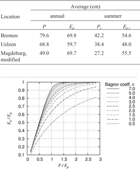
As the main advantage of Eq. (3) we would like to em-phasize its property to restrictEaeither to precipitation,P,or to potential evapotranspiration,Ep. Intermediate values of Eaare governed by the so-called Bagrov coefficientb. This parameter represents the availability of soil water to evapo-transpiration and depends on the amount of plant available soil water and capillary rise from groundwater. The Bagrov coefficient may vary between 0.5 for very restricted
availa-bility of soil water and about 8 for conditions of optimal evapotranspiration. The effect of b on actual evapotrans-piration is shown inFig. 1. This diagram could be used to evaluate Eq. (3) numerically. However, using the computer code provided is much more convenient.
There are two different conditions where the Bagrov method fails:
– because of the underlying assumption that infiltrated soil water be available to evapotranspiration,the method re-quires the residence time of infiltrated water in soil to be sufficient to make water available to evapotranspiration. This assumption is not met on sites with steep slope or with heavy storms on soils which exhibit at least tempora-rily an extremely high hydraulic conductivity,
– for plains under dry climatic conditions where the aquifer is recharged by groundwaterinflow from regions with pre-cipitation excess. Since Eq. (3) restricts actual evapo-transpiration to precipitation, it should not be used for wetlands whereEais enhanced by capillary rise from the groundwater table so much that it might exceed the local precipitation leading to groundwater depletion.
Both of these limitations require a different method to estimate actual evapotranspiration.
Location
Average (cm)
annual summer
P Ep Ps Ep,s
Bremen 79.6 69.8 42.2 54.6
Uelzen 68.8 59.7 38.4 48.0
Magdeburg, modified
49.0 69.7 27.2 55.5
T a b l e 3.Mean values ofPandEpat 3 locations(1961-1990)
RESULTS
The unknown parameter b may be estimated by a trans-fer function from data which are in general easily available. The best agreement between SWAP-simulated and Bagrov-estimated actual evapotranspiration was obtained by a trans-fer function of the form:
b c W c c q c C
P E
a
c s
s p s
= + +
-1 2 3 exp( 4 max) 5
,
, (4)
where: the variablesqmaxandCsare explained below,Psis precipitation,Ep,spotential evapotranspiration during sum-mer months (from April to September) and the coefficients c1...c5are fitting parameters.Wadenotes the maximum plant available soil water storage given by:
Wa=dr[ (q-63)- -q( 15850 ,)] (5)
where:dr– rooting detph (cm),q– soil water content as a fun-ction of soil water pressure head.
Parameters needed to evaluate Eq. (5) are shown in Tables 1 and 2. Please note thatWarepresents a soil and crop property which does not depend on evapotranspiration. In the context of this investigation, both of the pressure head values selected to represent field capacity and permanent wilting point are arbitrary variables to express correspond-ing soil hydraulic properties in Eq. (4). The detailed dis-cussion of field capacity is shown in Twarakavi (2009) and Zacharias and Bohne (2008) papers.
To consider the effect of capillary rise of water from the groundwater table to the root zone, an arbitrary steady-state flow rate,qmax, is chosen which approximates the maximum
flow rate to be expected under most conditions. The pressure head profile for any chosenqmaxis given (Bohne, 2005; Jury et al., 1991) as:
z( , )
( )
max min max
min
q h q
K h dh
h
= æ +
è
çç öø÷÷
ò 1
-0
1
, (6)
where: z – vertical coordinate, z = 0 at groundwater table (cm), q– flow rate (cm day-1),K(h) – unsaturated soil hydraulic con-ductivity (cm day-1),h– soil water pressure head (cm) and was calculated numerically. ForK(h), the van Genuchten-Mualem model of hydraulic conductivity was used (van Genuch-ten, 1980). A pressure value threshold ofhmin=-3 200 hPa
was chosen to obtain an approximate maximum capillary steady-state flow rate depending solely on soil hydraulic properties and flow distance,z. The advantage of this thres-hold is that data on unsaturated soil hydraulic conductivity to some extent are still available in this range (Rengeret al., 2009). Using Eq. (6) and soil hydraulic parameters as shown in Table 1, flow rates of texture classes were calculated. To bypass the processing of Eq. (6), an easy-to-use approxima-tion was prepared, which is given by:
qmax( )z = p z1 p2. (7)
The parametersp1andp2depend on texture class and
are shown in Table 4. Please note, that qmax describes steady-state maximum flow rates depending solely on soil hydraulic conductivity of the layer below the rooting zone and the flow distancezbetween the groundwater table and the lower boundary of the rooting zone without any regard to site, climate, and plant specific conditions.
Texture class p1 p2 Texture class p1 p2
Ss 1.524 103 -2.447 Uu 9.690 103 -2.100
Sl2 1.834 103 -2.383 Uls 2.766 103 -1.918
Sl3 5.875 103 -2.528 Us 1.948 103 -1.840
Sl4 5.183 102 -1.793 Ut2 3.835 103 -1.989
Slu 5.657 102 -1.721 Ut3 3.712 103 -1.986
St2 3.971 102 -1.497 Ut4 3.078 103 -2.008
St3 2.265 102 -1.804 Tt 6.213 101 -1.805
Su3 8.504 102 -1.742 Tl 9.920 101 -1.869
Su4 1.299 103 -1.736 Tu2 9.814 101 -1.864
Ls2 1.486 103 -1.586 Ts2 2.229 102 -1.963
Ls3 9.739 102 -1.794 Ts3 8.573 102 -2.103
Ls4 7.201 102 -1.766 Ts4 2.070 102 -1.520
Lt2 7.615 102 -1.762 fS 3.020 103 -2.481
Lt3 3.886 102 -1.671 mS 1.566 103 -2.454
Both of the influencing variables discussed so far describe the availability of soil water for evapotranspiration.
Actual evapotranspirationfurther depends on the
simulta-neity of atmospheric evapotranspiration demand and atmos-pheric water supply (Gluglaet al., 2003). If seasons with high potential evapotranspiration happen to be without rain-fall, actual evapotranspiration will be substantially lower than it would be in the case of evenly distributed rainfall. Based on thirty-year averages of monthly potential evapo-transpiration and precipitation a coefficient of simultaneity was established which is given by:
Cs
MAX E P
E
p i i
i
p i i
=
-å
å =
=
( , );
,
0
4 9
4
9 , (8)
where:PandEpdenote long-term averages of monthly sums
of precipitation and potential evapotranspiration, respec-tively. The expressionMAXstands for a function that re-turns the largest of the arguments given to it. The indexi de-notes the months from April to September.
To find the parameters of the transfer function Eq. (4) was substituted into Eq. (3) and the standard error of the predic-ted actual evapotranspitration was minimized by a FIBONACCI procedure (Vardavas, 1989). Integrations were performed
by the Simpson procedure and the implicit calculation ofEa
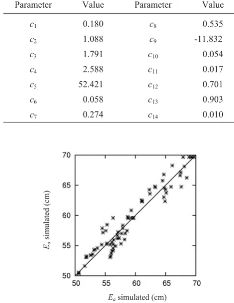
was done by the Newton algorithm. Because of the limita-tions of the Bagrov method as mentioned above, only two of the weather records were used to fit Eqs (3) and (4) to SWAP-generated data of actual evapotranspiration. The third re-cord, which was modified to represent semi-arid conditions, yielded substantial groundwater depletion and thus, a distur-bance of the local hydrological equilibrium. The results are shown inTable 5 and Fig. 2.Equation (3) predicts the actual evapotranspiration with a standard error of 1.55 cm.
The results discussed so far refer to soils without the in-fluence of anaerobiosis. For groundwater-affected clay soils
the Bagrov,b,parameter obtained from Eq. (4) should be
modified according to:
ba= -b c6(ha-c7)qcmax8 +c9qFC, (9)
where:hadenotes the soil water pressure head at the air
con-tent of 0.05 cm3cm-3,qFC=q(-63 hPa) is field capacity and bais the Bagrov coefficient corrected for anaerobiosis. The fitting coefficients,ci,are shown in Table 5. In the data base used are 15 data sets out of 135 showing anaerobiosis. The standard deviation betweenbaandbis 1.144.
If the long-term average of actual evapotranspiration exceeds precipitation, the limitations of the Bagrov method mentioned above require application of a different method. Based on the entire data base comprising 3 long-term wea-ther records, a statistic prediction equation was set up which is given by:
E
E c c P c q c W
a
p s
c
a
= 10+ 11 + 12 max13 + 14 . (10)
Equation (10) predicts the relationEa/Epusing the long-term average of summer precipitation,Ps(from April to September).
The remaining variables keep their meaning as explained above. It has been shown that during winter the difference between potential and actual evapotranspiration is
negligi-ble (Wessoleket al., 2011). Hence, from Eq. (1)
ground-water recharge,R,is obtained by:
R P E E E
E
p p s a
p
= - + æ
-è ç ç
ö ø ÷ ÷
, 1 , (11)
where:Ep,s– denotes the potential evapotranspiration
du-ring summer (from April to September).
The parameters of Eq. (11) are shown in Table 5. Equation (11) predicts groundwater recharge with an
stan-dard error of RMSE= 2.581 cm. Please note that this value
was obtained from the fitting procedure, not from applying
the method to an independent data set. The coefficient of
cor-relation between SWAP-simulated and predicted ground-water recharge is R = 0.975. Figure 3 displays results
Parameter Value Parameter Value
c1 0.180 c8 0.535
c2 1.088 c9 -11.832
c3 1.791 c10 0.054
c4 2.588 c11 0.017
c5 52.421 c12 0.701
c6 0.058 c13 0.903
c7 0.274 c14 0.010
T a b l e 5.Values of the fitting parameters of Eqs (4), (9), and (10)
Fig. 2.Comparison between simulated and estimated actual evapo-transpiration,Ea.
Easimulated (cm)
Ea
simulated
obtained from Eq. (11) vs. groundwater recharge. For Ea/Ep > 0.6 groundwater gets depleted. Because of high potential evapotranspiration, capillary water supply from groundwater is forced to meet the atmospheric demand.
CONCLUSIONS
1. The study has shown that it is feasible to estimate re-gional long-term groundwater recharge from easily avai-lable data. These are precipitation, potential evapotranspi-ration, soil texture and depth to groundwater.
2. There are two ways to estimate actual evapotrans-piration and groundwater recharge. If precipitation is higher than evapotranspiration, using the Bagrov method is sug-gested. This method is expected to yield reliable results under different conditions and its errors are tolerable. The method contains only one unknown parameter, which can be estimated by a transfer function. Since the Bagrov method restricts actual evapotranspiration to precipitation, it cannot be used for parts of catchments where long-term actual eva-potranspiration is in excess over precipitation. In this study, a purely statistic based method is provided to cover the general case.
3. The method described is meant for application in low-lands and its results need to be scrutinized.
4. It is expected that the method yields a reasonable first guess which may be improved by regional calibration.
REFERENCES
Allen R.G., Wright M.E., and Burman R.D., 1989.Operational estimates of evapotranspiration. Agron. J., 81, 650-662. Bohne K., 2005.An Introduction into Applied Soil Hydrology.
Catena Verlag Reiskirchen, Germany.
Bonta J. and Müller M., 1999.Evaluation of the Glugla method for estimating evapotranspiration and groundwater re-charge. Hydrol. Sci., 44(5), 743-761.
Glugla G., Jankiewicz P., Rachinow C., Lojek K., and Richter K., 2003.BAGLUVA - Wasserhaushaltsverfahren zur Bere-chnung vieljähriger Mittelwerte der tatsächlichen Verdun-stung und des Gesamtabflusses. Bundesanstalt für Gewäs-serkunde, Koblenz, Germany.
Glugla G. and Tiemer K., 1971.Ein verbessertes Verfahren zur Berechnung der Grundwasserneubildung. Wasserwirtschaft, Wassertechnik, 20(10), 349-353.
Jury W.A., Gardner W.R., Gardner W.H., 1991.Soil Physics. Wiley Press, New York, USA.
Kroes J.G. and van Dam J.C.(Eds),2003.Reference Manual SWAP version 3.0.3. Alterra Report, 773, Wageningen, the Netherlands.
Kroes J.G., van Dam J.C., Huygen J., and Vervoort R.W., 1999. Simulation of water flow, solute transport and plant growth in the Soil-Water-Atmosphere-Plant environment: User’s Guide od SWAP version 2. Technical Document Nr. 53 DLO Winand Staring Centre, Wageningen, the Netherlands. Luckner L., van Genuchten M.T., and Nielsen D.R., 1989.A
con-sistent set of parametric models for the two-phase flow of immiscible fluids in the subsurface. Water Resour. Res., 25, 10, 2187-2193.
Metselaar K. and de Jong van Lier Q., 2007.The shape of the transpiration reduction function under plant water stress. Vadose Zone J., 6, 124-139.
Renger M., Bohne K., Facklam M., Harrach T., Riek W., Schäfer W., Wessolek G., and Zacharias S., 2009. Boden-physikalische Kennwerte und Berechnungsverfahren für die Praxis. Bodenökologie Bodengenese, 40, 20-26.
Richter D.U., 1995. Ergebnisse methodischer Untersuchungen zur Korrektur des systematischen Messfehlers des Hell-mann-Niederschlagsmessers. Berichte des Deutschen Wetter-dienstes, 194, Offenbach, Germany.
Scheffer F. and Schachtschabel P., 1998.Lehrbuch der Boden-kunde. Ferdinand Enke Verlag, Stuttgart, Germany. Twarakavi N., 2009.An objective analysis of the dynamic nature of
field capacity. WRR45, W10410 doi: 10.1029/2009WR007944. Twarakavi N., Simunek J., and Schaap G., 2010.Can texture-based classification optimally classify soils with respect to soil hydraulics? Water Resour. Res., 46, W01501, doi:10.1029/2009WR007939.
van Dam J.C., Groenendijk K.P., Hendriks R.F.A., and Kroes J.G., 2008.Advances of modeling water flow in variably satu-rated soils with SWAP. Vadose Zone J., 7(2), 640-653. van Genuchten M.T., 1980. A closed-form equation for
pre-dicting the hydraulic conductivity of unsaturated soils. Soil Sci. Soc. Am. J., 44, 892-898.
Vardavas I.M., 1989.A Fibonacci search technique for model parameter selection. Ecol. Modeling, 48, 65-81.
Wessolek G., Bohne K., Duijnisveld W., and Trinks S., 2011. Development of hydro-pedotransfer functions to predict capillary rise and actual evapotranspiration for grassland sites. J. Hydrol., 400, 429-437.
Wessolek G., Duijnisveld W.H.M., and Trinks S., 2008. Hydro-pedotransfer functions (HPTFs) for predicting annual perco-lation rate on a regional scale. J. Hydrol., 356, 17-27. Zacharias S. and Bohne K., 2008. Attempt of a flux-based
evaluation of field capacity. J. Plant Nutr. Soil Sci., 171(3), 399-408.
Fig. 3.Groundwater recharge,R,vs. simulated and estimated rela-tionEa/Epunder arid climatic conditions.
R