Iranian Journal of Economic Studies
Journal homepage: ijes.shirazu.ac.ir
Gender and the Factors Affecting Child Labor in Iran: An Application of IV-TOBIT
Teimour Mohammadia,Zahra Karimi Mougharib, Sahand Ebrahimi Pourfaezb
a. Faculty of Economics, Allameh Tabataba’i University, Tehran, Iran.
b. Faculty of Economics and Administrative Sciences, University of Mazandaran, Babolsar, Iran.
Article History Abstract
Received date: 17 May 2017 Revised date: 14 December 2017 Accepted date: 18 December 2017 Available online: 20 December 2017
In this paper we first intend to examine the probability of falling into the realm of child labor by using the conditional probability theorem. Furthermore, we will compare the extent of each factor’s effect on boys and girls using a TOBIT regression model. Finally, we will analyze different aspects of Iran’s labor market to assess the future ahead of the children who are working at the moment. As the results will show, the probability of participating in the labor market conditional on belonging to the age group of 15 to 17 is 20.34 % for boys in comparison with girls that is 4.42 %. More probability scores are estimated in the paper. Moreover, the results from the TOBIT regression show that in general boys are more affected than the girls by the same factors. Also, based on the macro statistics published by Iran’s Statistical Center, the graduation of numerous people from graduate schools combined with the low and slow rate of economic growth makes it quite difficult to find a decent work in the country. As a result, the skilled labor force will be content with accepting low wage jobs which are more suitable for the unskilled workers. Therefore, those who left school earlier in their lives will face several problems in the future.
JEL Classification:
C34 I31 J83
Keywords:
Child labor Wealth paradox Luxury axiom TOBIT models Labor market
1. Introduction
ILO's 138 convention states that “any form of work that threatens a child's physical, mental or moral health” is considered child labor and hence must be
stopped. According to this definition, child labor includes a variety of forms. It could be done for hourly wages such as working in mines and factories; it could be done as free labor in family businesses such as family farms or even managing home chores such as taking care of the infants in the family so the mother could have more hours to work; or it could be done in forms of illegal activities such as prostitution and drug trafficking. The last for is what the ILO calls “The worst forms of child labor.”
[email protected]
Even though many countries signed this convention, one still finds that millions of children in developing nations are active in one or more types of child labor. Most studies consider poverty as the main reason behind such an event. When the parents' total earnings are not enough to make the ends meet, they become content with their children participating in the labor market. These studies claim, if given the choice, parents are reluctant to send their children to the labor market. This is known as the luxury axiom in the literature (Basu and Van, 1998). However, in households with family businesses, especially in the agriculture sector, the children possess a value as a free and reliable labor force. In other words, the marginal benefit of them participating in the family business surpasses the marginal benefit of them going to school. This is called the wealth paradox (Lima et al., 2015).
Besides the wealth paradox and the luxury axiom, there has been mention of other factors for child labor in the literature. In the presence of imperfect markets the demand for child labor as cheaper labor force increases (Dumas, 2013). Also lack of financial resources increases the tendency for supplying child labor (Bhalotra and Heady, 2003). In this case the children act as a form of insurance in the face of unexpected shocks. Some also consider inequality as a determining factor for child labor.
Before presenting solutions, one must fully understand the problem. Iran, as well as many developing nations lacks an official survey with emphasis on child welfare. Therefore, any attempt on assessing the state of child labor in Iran will have a considerable degree of error. Furthermore, many households hide their children’s activity status. Some because of shame, others simply don’t consider their children helping around the house or on the family farm as work. Hence, most of the data on child labor consists of truncated and censored observations. The most applicable survey in Iran for this purpose is the Households' Income - Expenditure Survey which has been conducted yearly since the late 1980s.
In this paper we extracted the information of children between the age of 7 and 17 years old. Our focus was on their personal characteristics such as age, gender, region and etc. as well as the household’s features such as the head's activity status, the head's gender and etc. using the conditional probability theorem we estimate the probability of a child participating in the labor market conditional on different personal and household features. Moreover, we apply a TOBIT model to assess the extent of different factor’s effect on child labor. For the purposes of comparison, we divided the data into two groups; boys and girls. Finally, by analyzing the combination of the labor force based on their education level, we presented a possible future for those who leave school and join the labor market earlier in their lives.
one can refer to Ranjan 2001). Also, among the studies which tried to take into account the indigeneity bias when estimating the TOBIT model – for instance, Keshavarz et al. (2014) – they applied a GMM method. This method solves the endogeniety problem. It however, keeps the truncation bias intact. In this paper we were able to apply an IV-TOBIT method which takes both problems into account. In other words, we tried to reach a more comprehensive result than the works done before on the matter.
The paper's structure is as follows. First a theoretical analysis of the reasons behind a child's choice to join the labor market is presented. Then the data and the estimation procedure will be discussed in more details. Afterwards, the probability of participating in the labor market conditional on different factors will be estimated. Moreover, a TOBIT regression will be estimated for boys and girls to give a point of comparison. Then the combination of the labor market in the period of 2006 - 2015 is analyzed. Finally, the concluding remarks are presented.
2. Theoretical Debate
2.1 Factors Affecting Child Labor
In most studies regarding child labor, the common belief is that when having alternatives, the parents are reluctant to send their children to the labor market. Bandera et al. (2014) have covered this argument in their work. According to such studies, the head of the family is considered an altruist. However, some studies beg to differ (Bhalotra and Heady, 2003; Kambhampati and Ranjan, 2006; Dumas, 2007; Kruger, 2007; and Lima et al., 2015). Basu and Van (1998) were the first to put emphasis on this argument by designing a household’s decision making model. In the literature this phenomenon is known as the luxury axiom. Based on the luxury axiom, given all other conditions are constant, parents prefer their children not to participate in the labor market. On the other we have the wealth paradox.
the first effect is known as the income effect (Basu and Van, 1998) and the second is known as the substitution effect (Bhalotra and Heady, 2003; Kambhampati and Ranjan, 2006; Dumas, 2007; Kruger, 2007; and Lima et al., 2015). However, the rate of altruism among household members (Fan, 2011) and their bargaining power (Keshavarz et al., 2014; Keshavarz and Borhani, 2012) affects the extent of income and substitution effects. The wealth paradox is also observable in non – farmer households where child labor is supplied. In this case, increase in parents’ hours of work means increase in their workload. In here the child plays the role of a cheap potential worker, hence the substitution effect exists .
Despite the disagreement regarding the supply of child labor in rural households with land property which has low liquidity rates (Lima et al., 2015), some agreements do exist. The most common reason for the existence of child labor which many agree upon is poverty (Basu and Van 1998; Bandera et al., 2014). The poor are more vulnerable in the face of economic and natural shocks (Landmann and Frolich, 2015). Therefore, these households show higher tendencies to supply child labor. Furthermore, economic shocks are themselves considered an affecting factor for the existence of child labor (Duryea et al., 2007; Dillon, 2013; Beegle et al., 2006). Households seek ways to mitigate the effects of economic shocks. Child labor is one of these ways (Cain, 1982; and Portner, 2001) that in the absence of alternatives such as social insurance (Landmann and Frolich, 2015), access to financial resources (Bandera et al., 2014) and properties with high rates of liquidity (Beegle et al 2008; Binswanger and McIntire, 1987) becomes more common among poor households. This has been examined quite often in the literature (Cu Ravallion and Chadhuri, 1997; Townsend, 1994; Zeldes, 1989; and Morduch, 1999).
2.2 Household’s Decision Making Model
When modeling the household’s behavior regarding the supply of child labor, most studies use an overlapping generation analysis (Cf Ranjan, 1999; and Pallage and Dessy, 2001). However, in some studies the decision to supply child labor is studied in one period and based on the household’s consumption incentives (Basu and Van, 1998; Basu et al., 2009). In this study we apply the former.
2.2.1 The Model’s Assumptions
The model’s assumptions are as follows:
- There is one household in the model consisting of a child and an adult;
- The model has two periods of 0 and 1;
- In the first period there is a child and an adult in the household;
- In the second period the adult has passed away and the child has become an adult;
- There are 3 forms of labor; skilled, unskilled and child labor;
- The unskilled labor earns a wage less than the skilled and more than the child;
- The difference between the skilled and unskilled worker’s earning is due to the difference between their efficiencies;
- The difference between the child and the unskilled labor’s earnings is due to the difference between their labor supplies.
2.2.2 The Household’s Decision Making
The household has the following utility function:
where C0 is the consumption in the first period, C1 is the consumption in the second period, is the rate of risk aversion and is the rate of time discount. Here the household seeks to maximize its total utility. Furthermore, the consumption in any of the periods cannot exceed the net income of the respective period.
For simplicity we assume that a household with a skilled adult, does not supply any child labor. This has been supported by the literature (Ranjan, 2001). The maximizing problem in front of the household is as follows:
where I0 and I1 are the income from work in the first and second periods. b is the household’s initial endowment in the first period and S0 is the household’s savings in the first period which will be spent in the second period. Furthermore, the household’s total endowment will be spent in the first period. Whether the household supplies child labor or not, Ii will have different values in the first and second periods:
{
{
where w is the market’s base wage, is the unskilled worker’s efficiency, L is the amount of labor supply, 0 and 1 are the indictors for the two periods, C and
A are respectively indicators for the child and the adult and is the efficiency of the skilled worker.
2.2.2.1 Scenario 1 ( )
In this case the household intends to maximize its lifespan utility given the constraints that the consumption in each period does not exceed the net earnings of the household in that period. Therefore:
In order to solve the optimization problem, we have two methods. One is to use the Lagrange Multiplier method. The other method is the fact that the marginal benefit for an extra unit of consumption in the first period must be equal to the marginal dis-benefit for a less unit of consumption in the second period in order to maximize the total utility of the households. Therefore:
[ ]
[ ]
[ ]
Rewriting the equation 10 gives us the equation 12 which is the rate of consumption exchange between the two periods. Using two simplifying assumptions, we can extract the initial endowment for not supplying child labor and the market wage in the absence of child labor. Assume that the household’s consumption is constant in the two periods and equals to 1. Also, in each period the adult supplies 1 unit of labor. Therefore:
[ ]
[ ]
b*in equation 17 is the equilibrium endowment when the household does not supply any child labor. It is worth noting that in this case not supplying child labor in the first period means the household’s child attends school or training and hence the household’s labor in the second period will be a skilled worker. Therefore, in the second period the household’s earnings from the labor’s income will exceed its income in the first period due to the higher efficiency of the skilled worker (1<Γ) in comparison with the unskilled labor (0<γ<1). Solving the equation 15 for w gives us the equilibrium wage in the first scenario: [ ]
[ ]
2.2.2.2 Scenario 2 ( )
In the second scenario the household, instead of accumulating human capital, decides to supply child labor in the first period. In this case, the household will maximize the equation 1 (total utility) subject to new constraints:
This time, in the first period the earnings from the child’s work will be included besides the unskilled adult worker’s earnings in the constraint for this period. Furthermore, since the child did not attend any form of education or training in the first period, the earnings from the labor supply in the second period will be for an unskilled worker. In this case, like the first scenario, we could extract the equilibrium values. Marginal benefit of an extra unit of consumption in the first period must be equal to the dis-benefit of a less unit of consumption in the second period. Therefore:
[ ]
[ ]
This time the rate of exchange for consumption between two periods will be the equation 24 which is more than the same ratio in scenario 1. In here, by assuming the equations 13 and 14 we can extract the child’s labor supply:
[ ]
[ ]
adult’s inadequate income. Therefore, the child only works as much as is needed and hence more wages mean less hours of work. In the literature this is called the poverty hypothesis (Dumas, 2013). However, in the presence of imperfect markets (Dumas, 2015) or the absence of alternatives (Landmann and Frolich, 2015; Bandera et al., 2014), the child’s leisure will be considered a luxurious good and therefore until a higher income threshold is reached the relationship remains positive (Dumas, 2013). Next we enter two more simplifying assumptions. First, we assume that in the second scenario the household lacks any initial endowment. Moreover, we assume that the household has no savings in the first period. In other words:
The reason for assumptions 28 and 29 are quite simple. According to the literature, the main objective behind the supply of child labor is to compensate for the inadequacies of the adults’ income in meeting the household’s consumption needs (Basu and Van, 1998; Ersado, 2005; and Kruger, 2007). In this case, lack of endowment and savings gives a more realistic model:
( ) Also:
[ ]
Comparing the market wage in the presence of child labor (wc) and in its absence (w*) shows that the existence of child labor can result in lower market wages.
3. Methodology and Data 3.1 Data
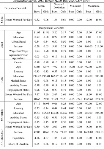
The data source for this study is the households’ income – expenditure survey conducted in 2013. This survey covers 140,359 individuals. We extracted the information for people with more than 6 and less than 18 years of age (24,903 individuals). 81 individuals where omitted due to lack of sufficient data. The descriptive statistics are presented in table 1.
Table 1. The Descriptive Statistics (Extracted from the Households' Income - Expenditure Survey, 2013, Include 11,335 Boys and 10,677 Girls)
Dependent Variable Mean
Standard
Deviation Minimum Maximum
Boys Girls Boys Girls Boys Girls Boys Girls
C
hi
ld
Hours Worked Per Day 0.32 0.06 1.54 0.61 0.00 0.00 12.00 15.00
Independent Variables
C
hi
ld
Age 11.95 11.86 3.20 3.17 7.00 7.00 17.00 17.00
Education 0.92 0.88 0.27 0.32 0.00 0.00 1.00 1.00
Urban/Rural 0.54 0.54 0.50 0.50 0.00 0.00 1.00 1.00
Income 0.28 0.05 5.89 2.28 0.00 0.00 460.00 219.00
Wage/NonWage 1.93 1.98 0.34 0.19 0.00 0.00 1.00 1.00
Agriculture/ Non
Agriculture 0.03 0.01 0.19 0.12 0.00 0.00 1.00 1.00
H
E
A
D
Gender 0.98 0.98 0.13 0.13 0.00 0.00 1.00 1.00
Age 43.03 42.78 7.92 8.18 18.00 18.00 99.00 92.00
Literacy 0.83 0.83 0.37 0.37 0.00 0.00 1.00 1.00
Education 197.22 196.48 162.79 161.66 0.00 0.00 905.00 905.00
Marital Status 0.98 0.98 0.13 0.13 0.00 0.00 1.00 1.00
Activity Status 0.98 0.98 0.14 0.13 0.00 0.00 1.00 1.00
Employment Status 0.96 0.96 0.20 0.19 0.00 0.00 1.00 1.00
Hours Worked Per Day 7.57 7.60 2.67 2.66 0.00 0.00 18.00 18.00
Income 40.66 39.35 73.49 70.61 -6.85 -27.0 1599.60 1599.60
M
O
T
H
E
R
Age 37.17 36.93 9.06 9.25 0.00 0.00 90.00 72.00
Literacy 0.75 0.74 0.44 0.44 0.00 0.00 1.00 1.00
Education 157.0 155.12 145.28 144.62 0.00 0.00 905.00 905.00
Activity Status 0.15 0.15 0.36 0.36 0.00 0.00 1.00 1.00
Employment Status 0.15 0.15 0.36 0.36 0.00 0.00 1.00 1.00
Hours Worked Per Day 0.80 0.80 2.07 2.06 0.00 0.00 15.00 15.00
H
O
U
S
E
H
O
L
D
Income 42.03 40.68 73.96 71.22 0.00 0.00 1608.83 1608.83
Population 4.76 4.87 1.35 1.40 1.00 1.00 13.00 13.00
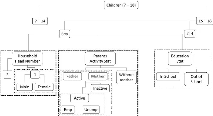
Figure 1. The Primary Decision Tree for Participation in the Labor Market
After extracting the data on children between the ages of 7 and 17 years old, we divided them into two categories; those who are economically active and those who are not. To take a closer look at the factors defining their choice, we defined a cluster of micro level factors, namely the characteristics of the child and his or her household. Finally, using the conditional probability theorem, we estimated the probability of a child participating in the labor market conditional on his or her personal and household characteristics. For instance, the probability of a child participating in the labor market conditional on his or her gender is estimated as stated in the following:
|
In other words, the probability of a child participating in the labor market conditional on him being a boy, is estimated by dividing the probability of participating in the labor market and being a boy by the probability of being a boy. Based on the different characteristics that the child may have, we designed a decision tree (figure 1).
3.2 The Methodology 3.2.1 The TOBIT Model
importance, then multiple regressions will be consistent. However, when faced with such data, both procedures will be biased. Because it matters that with what probabilities the observations are above or below the limit and also it is important to know what absolute values they take. In econometrics this form of bias is called the truncation bias or the censored data bias. In this case the dependent variable takes the following form:
{
In other words, the dependent variable whether takes non negative values of or 0. In the above equation system follows the following regression model:
In this paper we focus on factors that besides affecting the household’s decision on children’s participation in the labor market, also has effect on the hours the children work. We use the micro data from the Households’ Income – Expenditure Survey. Since a considerable number of households hide the activity status of their children, the data faces the problem of censored data. Due to the two sided nature of our objective and also because of the possibility of censored data, applying the TOBIT model seems to be the best estimation procedure.
The estimated equation in our study will be as follows:
{
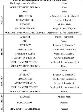
Table 2. The Independent Variables Used in the Model
The Independent Variables Units
C
H
IL
D
HOURS WORKED PER DAY Hour
AGE Years
EDUCATION In School: 1, Out of School: 0
URBAN/RURAL Urban: 1, Rural: 0
INCOME Million Rials
WAGE/NONWAGE Wage: 1, Non-Wage: 0
AGRICULTURE/NONAGRICULTURE Agriculture: 1, Non-Agriculture: 0
H
E
A
D
GENDER Male: 1, Female: 0
AGE Years
LITERACY Literate: 1, Illiterate: 0
EDUCATION The Level of Education
MARITAL STATUS Married: 1, Single: 0
ACTIVITY STATUS Active: 1, Inactive: 0
EMPLOYMENT STATUS Employed: 1, Unemployed: 0
HOURS WORKED PER DAY Hours
M
O
T
H
E
R
AGE Years
LITERACY Literate: 1, Illiterate: 0
EDUCATION The Level of Education
ACTIVITY STATUS Active: 1, Inactive: 0
EMPLOYMENT STATUS Employed: 1, Unemployed: 0
HOURS WORKED PER DAY Hours
H
O
U
S
E
H
O
L
D INCOME Million Rials
POPULATION Persons
SHARE OF THE CHILDREN Percent
4. Estimation Results
4.1 The Conditional Probabilities
probability of participating in the labor market conditional on the child’s different characteristics. It is worth noting that the probability formula gives us the labor force participation rates. For instance, the probability of a boy participating in the labor market conditional on his age will be the number of boys in the specific age group who are active divided by the number of boys in that age group. As one can see, this is the same as the participation rate for boys in a specific group.
Given the results, age has a considerable effect on the probability of a child participating in the labor market. As can be seen in Figure 2 the probability for the age of 15 to 17 years is considerably higher than for the age of 7 to 14 years. This is in accordance with the tendency of many researchers in the field to use the square of age besides age itself in their studies.
On the other hand, the probability of participating in the labor market among boys is considerably higher than among girls. This holds for the both age groups. This indicates that in higher ages, children’s tendency to enter the labor market also rises. Also, it is noteworthy to mention the great increase in the gap between girl’s and boy’s probabilities, especially at the age group of 15 to 17. This in turn indicates the fact that boys have a higher tendency to participate in the labor market instead of keeping with their studies.
Figure 2. The probability of participating in the labor market conditional on age
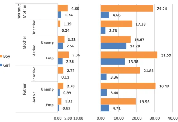
Since the great difference among children between the age group of 7 to 14 with the age group of 15 to 17 we divided the children into the two age groups. The figures on the left are for the age group of 7 to 14 and the figures on the right belong to the age group of 15 to 17.
As one can see in figure 3, the probability of participating in the labor market is higher in one headed households. Results also indicate that one headed households with male heads are more content with their children participating in the labor market.
The probability of participating in the labor market for the age group of 15 to 17 is considerably higher than the age group of 7 to 14. Moreover, in both groups, the probability of boys’ participation is higher than girls. However, the
0.61 4.42
1.94
20.34
0.00 5.00 10.00 15.00 20.00 25.00
7_14 15_18
Boy
gap widens with increase in age. That is partly because in higher ages, boys and girls take different paths with the former participating in the labor market and the latter participating in household unpaid chores or getting married.
Figure 3. The probability of participating in the labor market conditional on households head numbers
The parents’ activity status has also a considerable effect on the children’s participation in the labor market. The probability of a child participating in the labor market conditional on the mother being employed is higher in both age groups and for both the genders. This indicates that the economically active children are usually working with their mothers. The considerable difference in the numbers between the two age groups and the increase in the gap between the two genders again indicate the results we mentioned earlier.
Figure 4. The probability of participation in the labor market conditional on parent's activity status 8.33 0.69 0.55 10.77 2.59 1.86
0.00 10.00 20.00 30.00 40.00 Male Female 1 2 Boy Girl 11.43 4.52 4.34 34.29 30.00 19.71
0.00 10.00 20.00 30.00 40.00
0.65 0.99 0.11 2.36 2.56 0.24 1.74 1.81 2.70 2.74 5.36 3.23 1.19 4.88
0.00 5.00 10.00 Emp Unemp Emp Unemp A ct iv e In ac ti ve A ct iv e In ac ti ve Fa th er M o th er W it h o u t M o th er Boy Girl 4.71 3.40 3.36 13.38 14.29 2.73 4.66 19.56 30.43 21.83 31.59 16.67 17.38 29.24
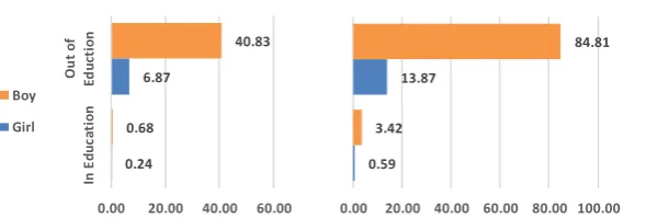
According to Figure 5 the probability of participating in the labor market conditional on leaving school is considerably high. This holds for both the age groups. Furthermore, this probability is quite higher for boys in respect to girls. The gap increases with age. Also, the participation in the labor market after leaving school in the age group of 15 to 17 is almost definite. The higher gap between boys and girls in the age group of 15 to 17 supports our prior conclusion. Girls are more prone to leave school for marriage or participation in unpaid house chores.
Figure 5. The probability of participating in the labor market conditional on education status
4.2 The IV-TOBIT Results
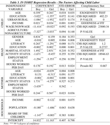
In this paper we divided the data into two groups; girls and boys. This division was to compare the extent of each variable’s effect on each gender. According to the results (Table 3) the null hypothesis for exogeneity is rejected for the first model (boys) with a 99 % degree of confidence. However, the same cannot be said for the second model (girls). Since the null hypothesis was not rejected, we did not apply the instrumental method for the second model. Also, the mother’s employment status arose the problem of convergence. Therefore, it was omitted from the estimation.
In both models increase in age has a significant positive effect on the probability of working and the hours worked. However, this effect is stronger in boys (0.359) in comparison with girls. Attending school decreases the probability of working and the hours worked. Again the effect in the first model (-3.022) is stronger than the second (-1.357). Living in urban areas decreases the hours worked given they work. However, this time the effects in the first model (-1.084) are weaker than the second (-1.952). The results of the estimations reject the poverty hypothesis in both models. As will be shown in the next section that is mainly because of imperfections in the labor market. Having wage jobs has a negative effect on the dependent variable. The difference between boys and girls is not considerable here. Working in agriculture has also a negative effect on the hours worked given they work. The effects for boys (-7.327) is much stronger than for girls (-3.033) .
0.24 6.87
0.68
40.83
0.00 20.00 40.00 60.00
In
E
d
u
ca
ti
o
n
O
u
t
o
f
Ed
u
ct
io
n
Boy
Girl
0.59 13.87
3.42
84.81
Table 3. IV-TOBIT Regression Results - The Factors Affecting Child Labor
INDEPENDENT VARIABLE
COEFFICIENT STD-ERROR Complimentary Stat
Boy Girl Boy Girl Boy
C
H
IL
D
AGE 0.359*** 0.263*** 0.018 0.035 EXOGENEITY TEST
EDUCATION -3.022*** -1.357*** 0.072 0.141 CHI-SQUARED 402.23
URBAN/RURAL -1.084*** -1.952*** 0.073 0.174 P-VALUE 0
INCOME 0.021*** 0.034*** 0.001 0.003 GOODNESS of FIT
WAGE/NONWAGE -11.414*** -10.023*** 0.092 0.193 CHI-SQUARED 23880.34
AGRICULTURE/
NONAGRICULTURE -7.327
***
-3.033*** 0.094 0.148 P-VALUE 0
H
E
A
D
GENDER 0.834*** 0.159 0.184 0.353 Girl
AGE -0.010** 0.005 0.004 0.008 EXOGENEITY TEST
LITERACY 0.263*** -1.291*** 0.088 0.171 CHI-SQUARED 1.2
EDUCATION -0.002*** 0.002*** 0.000 0.001 P-VALUE 0.2737
MARITAL STATUS 1.492*** 2.831*** 0.210 0.352 GOODNESS of FIT
ACTIVITY STATUS -1.671*** -0.457 0.255 0.359 CHI-SQUARED 18946.63
EMPLOYMENT
STATUS -1.294
***
-3.353*** 0.256 0.359 P-VALUE 0
HOURS WORKED
PER DAY 0.170
***
0.192*** 0.013 0.024 Pesudo R2 0.667
M O T H E R
AGE -0.024*** -0.039*** 0.004 0.008
LITERACY 0.131 -0.313* 0.091 0.177
EDUCATION -0.001* -0.002*** 0.000 0.001
ACTIVITY STATUS 1.731*** -4.279*** 0.527 0.273
EMPLOYMENT
STATUS -3.439
***
- 0.542 -
HOURS WORKED
PER DAY 0.244
***
0.567*** 0.023 0.036
H O U S E H O L
D INCOME -0.002*** 0.122* 0.001 0.075
POPULATION -0.180*** -1.686** 0.043 0.638
SHARE OF THE
CHILDREN -1.147
**
-0.003** 0.383 0.001
INTERCEPT 14.832*** 11.163*** 0.407 0.798
Note: *** 99 % degree of confidence ** 95 % degree of confidence * 90 % degree of confidence
(1.492 for boys and 2.831 for girls). It seems though that the girls take a bigger hit from this variable. An active head of household decreases the de pendent variable by 1.671 points for boys. However, it has no significant effects on girls. On the other hand, being employed has a strong negative effect on the hours worked given they work in both models. The effect for girls ( -3.353) is much stronger than for boys (-1.294). The relationship between the hours worked given they work and the hours worked by the head of the household are significant and positive in both models. The difference between the two is not considerable.
Increase in mother’s age decreases the dependent variable in both models (-0.024 for boys and -0.039 for girls). The difference is not considerable. The mother’s literacy shows no significant effect for boys however it has a negative effect for girls (-0.313) with 90 % degree of confidence.
The effect of mother’s education level is significant and negative for both models. However, its value is negligible. Interestingly the coefficient for the mother’s activity status is positive for boys and negative for girls. In other words, when the mother is active the girl’s work will mainly consist of home chores and domestic works. The mother’s employment status was omitted from the second model due to the problem of convergence. It however, has a negative significant effect of the dependent variable for the boys. The more the mother works, the more the children who work participate. This is in par with the wealth paradox .
The household’s income shows a negative effect in the first model. However, its effect is not statistically significant in the second model. The small value of this coefficient is partly due to the largeness of the variable in comparison with the dependent variable. In the more populated households the probability of a child’s work or his/her amount of work decreases. The effect for girls (-1.686) is much stronger than for boys (-0.180). The proportion of children to adults has also a negative effect. This time, the effect for boys (-1.147) is much stronger than for girls.
4.2 The Future of the Out of School Children in Iran’s Labor Market
The data for this part of the paper has been extracted from Iran’s Survey on Labor Market. This survey is conducted seasonally and focuses on Iranian’s employment aspects. We mentioned earlier that in imperfect labor markets the employment options for those who choose work instead of schooling in their earlier periods of life will be limited during their adulthood. According to the data presented here, this may very well be the case in Iran’s labor market.
education (32.87 %) and higher education (20.93 %) increased considerably. By the year 2015, highly educated work force had the highest share (42.24 %) among the unemployed population .
In 2006 the highest share of inactivity belonged to those with higher levels of education (24.26 %). By the year 2015 this share declined to 14.25 %. However, the absolute numbers paint a more drastic picture. The total population of the country in 2015 who were economically active was around 25 million people. The number of the inactive population is about 40 million persons. With a closer look one can see that the number of active population with higher education (around 6 million) is as much as the number of inactive persons with higher education (more than 5 million).
Iran economy is now in a state of recession. After two years of negative rates, the GDP has reached a growth rate of 1.88 % in 2014. On the other hand, the rate of unemployment is as high as 12 %. This rate is twice as high when estimated for the youth. Furthermore, the participation rate in 2015 was 38.18 %. When accounting for gender the rate becomes more significant. Female participation rate was 13.25 % and male participation rate was 63.21 %. In other words, the employment opportunities in the economy are quite slim. Also, a vast majority of the population have left the labor market and attended the universities in the hopes of better jobs in the future.
Unfavorable labor market conditions will have negative effects on the future of the children who have chosen work instead of school in their early ages. The economy at its current state is incapable of cre ating jobs for the vast number of highly skilled workers who will soon graduate from universities. Therefore, those who do not find the employment they desire and are not able to migrate to countries with better job opportunities, inevitably will accept unskilled, low paid jobs in Iran. In other words, the blue color job vacancies will be filled by the higher educated work force; as employers will prefer to hire them instead of illiterate or low skilled workers who left school in their childhood. At the moment a large proportion of semi-skilled and low skilled jobs such as taxi drivers, store salesmen, and factory guards have bachelor or higher degrees. It is highly probable that in the near future, illiterate laborers and workers with low literacy levels will get the lowest paid, insecure jobs. So, the chance to get out of the poverty trap will be very slim for the children who leave schools in their early ages. In other words, they and their households might fall into a vicious circle of poverty.
5. Concluding Remarks
working more than 8 hours a day. In here we attempted to shed some light on the reasons behind such events .
The purpose of our paper was to study the extent of different personal and household characteristics and their effects on the probability of a child entering the labor market and the amount of work he/she has to endure. In order to do so, we extracted the micro data on 24,822 children between the ages of 7 and 17 years old. Our focus was on their personal and household features. The data are extracted from the yearly Households’ Income – Expenditure Survey that is published by Iran’s Statistical Center .
According to the data, 2,470 children out of the 24,822 children were not enrolled in any form of schooling. Among them 41.54 % were male; 7.65 % lived in one headed households; 8.7 % were between 7 to 10 years old; 57.1 % were between 10 to 15 years old; 34.25 % were between 16 to 17 years old; 91.2 % lived in male headed households; 36.8 % were economically active; 27.33 % resided in urban areas; 83.72 % had an active father and 16.8 % had an active mother.
Then we estimated the conditional probabilities for children participating in the labor market conditional on different factors such as their gender or the activity status of their parents. Based on the results, by the increase in age the probability of a child participating in the labor market increases as well. Furthermore, being in a one headed household increases the probability of participation in the labor market. Moreover, there is a considerable gap between boys’ and girls’ probability of participation in the labor market. This gap widens with increase in age in favor of boys. This is partly due to the fact that girls mostly tend to participate in unpaid house chores and also their tendency to get married increases with age.
Afterwards, applying a TOBIT regression model, we presented a comparison between the determining factors for boys and for girls. In the model for boys the exogeneity hypothesis was rejected. Therefore, we used the head of household’s net income as an instrument for the household’s net income. The test was not rejected for girls and hence the second model was estimated without any instrumental variables. Also, the mother’s employment status was omitted in the second model due to the problem of convergence.
According to the results, boys’ personal characteristics in general have stronger effects on the hours worked given they work in comparison with girls. For instance, the coefficient for education in boys is almost 3 times the coefficient for girls. Furthermore, the head of household’s literacy shows different effects between the boys and the girls. This difference is in favor of the girls. However, with improvement in the head’s education level the balance shifts towards the boys. Moreover, the characteristics of the mother have stronger effects on girls. On the other hand, the share of children in a household works in favor of the boys.
educated labor force has increased significantly in the past two decades. University educated work force hope to find white color jobs that are related to their set of skills. However, in a labor market with about 12 % unemployment rate, more than 20 % youth unemployment rate and around 50 % participation rate, the future does not seem so optimistic. In the coming years the number of active population with higher education levels will face a big boom. However, there are not as much vacancies in the high wage, formal sector .
References
Bandara, A., Dehejia, R., & Lavie, S. (2014). Impact of income and non-income
shocks on child labor, Working Paper No 118. Retrieved from United
Nations University: http://www.wider.unu.edu/
Basu, K., & Van, P. H. (1998). The economics of child labor. American
Economic Review, 88(3), 412-427.
Beegle, K., Dehejia, R. H., & Gatti, R. (2006). Child labor and agricultural shocks. Journal of Development Economics, 81(1), 80-96.
Beegle, K., Dehejia, R., Gatti, R., & Krutikova, S. (2008). The consequences of
child labor: Evidence from longitudinal data in rural Tanzania. Washington, DC: World Bank.
Bhalotra, S., & Heady, C. (2003). Child farm labor: The wealth paradox. The
World Bank Economic Review, 17(2), 197-227.
Binswanger, H. P., & McIntire, J. (1987). Behavioral and material determinants
of production relations in land-abundant tropical agriculture. Economic
Development and Cultural Change, 36(1), 73-99.
Cain, M. (1982). Perspectives on family and fertility in developing countries. Population Studies, 36(2), 159-175.
Dillon, A. (2012). Child labor and schooling responses to production and health shocks in northern Mali. Journal of African economies, 22(2), 276-299. Dumas, C. (2007). Why do parents make their children work? A test of the
poverty hypothesis in rural areas of Burkina Faso. Oxford Economic Paper,
59(2), 301-329.
Dumas, C. (2013). Market imperfections and child labor. World Development,
42(1), 127-142.
Dumas, C. (2015). Shocks and child labor, Working Paper No 458. Retrieved
from Université de Fribourg: http://doc.rero.ch./
Duryea, S., Lam, D., & Levison, D. (2007). Effects of economic shocks on
children's employment and schooling in Brazil. Journal of development
economics, 84(1), 188-214.
Ebrahimi-Pourfaez, S. (2012). The Status of Decent Work Indicators among
Chosen Developing Countries. Master’s Thesis. Faculty of Economics. University of Mazandaran.
Ersado, L. (2005). Child labor and schooling decisions in urban and rural areas:
Comparative evidence from Nepal, Peru, and Zimbabwe. World
Development, 33(3), 455-480.
Fan, C. S. (2011). The luxury axiom, the wealth paradox, and child labor. Journal of Economic Development, 36(3), 25-45.
Kambhampati, U. S., & Ranjan, R. (2006). Economic growth: A panacea for child labor? World Development, 34(3), 426-445.
Individual Labor Supply in Iran. Journal of Economics Studies, (4)47, 155 – 177 [In Persian].
Keshavarz-Haddad, G., Nazarpour, M., & Seifi-Kafshgari, M. (2014). Child Labor among Iranian Households. Economic Policies, University of Mofid, 7(26), 125 – 143 [In Persian].
Kruger, D. I. (2007). Coffee production effects on child labor and schooling in rural Brazil. Journal of Development Economics, 82(2), 448-463.
Landmann, A., & Frölich, M. (2015). Can health-insurance help prevent child
labor? An impact evaluation from Pakistan. Journal of Health Economics,
39(1), 51-59.
Lima, L. R., Mesquita, S., & Wanamaker, M. (2015). Child labor and the wealth paradox: The role of altruistic parents. Economics Letters, 130(1), 80-82. Morduch, J. (1999). Between the state and the market: Can informal insurance
patch the safety net? The World Bank Research Observer, 14(2), 187-207.
Pörtner, C. C. (2001). Children as insurance. Journal of Population Economics,
14(1), 119-136.
Ranjan, P. (2001). Credit constraints and the phenomenon of child labor. Journal of Development Economics, 64(1), 81-102.
Ravallion, M., & Chaudhuri, S. (1997). Risk and insurance in village India: Comment. Econometrica, 65(1), 171-184.
Tobin, J. (1958). Estimation of relationships for limited dependent variables. Econometrica, 26(1), 24-36.
Townsend, R. M. (1994). Risk and insurance in village India. Econometrica,
62(3), 539-591.