Projection Space Maximum A Posterior Method
for Low Photon Counts PET Image
Reconstruction
Liu Zhen
Computer Department / Zhe Jiang Wanli University / Ningbo
ABSTRACT
In this paper, we proposed a new MAP method more suitable for low signal to noise (SNR) measurements. Different from conventional MAP method, we assume the projection space as a Gibbs field and the penalty term we used was defined in projection space. The spatial resolution of our method was studied and we furthermore modified our method to obtain nearly spatial invariant resolution. Both simulated data and real clinical data were used to testify our method, and future work was discussed at the end of the paper.
Keywords: PET, image reconstruction, MAP, Gibbs, local impulse response
I. INTRODUCTION
PET image reconstruction problem is an ill posed inverse transform (ill-posed), tiny disturbance observation data reconstruction results may lead to a serious distortion, so often need to adopt regularization method to improve the reconstruction quality. The most common one is the maximum posterior probability density (MAP) algorithm based on Bayes estimation, [1-7]. In MAP algorithm, the distribution rule of image space usually takes the form of prior function as regular item, and the algorithm is constrained. Different prior functions have different effects on reconstruction results. However, for the convenience of computation, people often limit their influence range to a smaller neighborhood when constructing a priori function. This definition is based on prior distribution function, often local features in the image is more sensitive, but the overall characteristics of the image is not well described, so the reconstruction of high noise observation data, the results are often not ideal. Although the weight of the prior function can be increased by modifying the super parameter (hyper parameter), the binding of the prior function to the algorithm can be enhanced, but it may lead to instability of the algorithm.
In this paper, we propose a new reconstruction method for high noise pollution observation data, which is called projection space maximum posterior probability density algorithm. Unlike the traditional MAP algorithm, we consider the projection space (the Radon transform space of the image) as a Gibbs random field, and construct a prior distribution function in this space. This transcendental function definition fully considers the overall features of the image, the neighborhood system is equivalent to the definition in the image space of non local and global, in the case of high noise convergence for the algorithm provides effective binding.
For the traditional MAP algorithm, even if the spatial invariant (space-invariant) projection method and the spatial invariant penalty term are used, the reconstructed results may still have non-uniform spatial resolution related to objects. Fessler Made a detailed study of this phenomenon and proposed several methods to correct the spatial resolution characteristics of the reconstructed results[8-11]. In this paper, a similar method is used to correct the projection space prior function in order to obtain approximately consistent image spatial resolution.
and proposed that different sub parameters were selected according to the area of the reconstructed object, so that different resolutions of [9, 11, 14] were obtained in different regions of the image. Qi proposes another method of selecting hyper parameters, [15, 16]. He used the contrast recovery coefficient (CRC: Contrast Recover y Coefficient) to describe the spatial resolution characteristics of the image, and the noise contrast (CNR: Contrast to Noise Ration) as a function of the observed variables, by modifying the parameters to maximize the CNR, this method realizes automatic selection of hyper parameters, and obtain approximate consistent spatial resolution. In this paper, we use the maximum likelihood estimation (ML: Maximum Likelihood) method to select the global hyper parameter. Zhou has applied this method to the selection of [17] parameters in MAP estimation, but its drawback lies in the large amount of computation. However, the projection space priors proposed in this paper can effectively reduce the computational complexity of ML estimation.
This paper is organized as follows: in section second, first reviewed the MAP estimation model, and then puts forward the projection space prior function method is proposed to modify the spatial resolution, after that, we discuss the selection of hyper parameters. In the third section, the reconstruction effect of the algorithm is analyzed and compared by using simulated data and real projection data. Finally, the algorithm is summarized and discussed.
II. RECONSTRUCTIONALGORITHM
A. MAP reconstruction model
As { }
i y
=
y as the observation data, the parameters q = {qj}to be estimated are defined ,yand qdefined in the
observation data space Y and parameter space Q respectively. According to the Bayes formula, the MAP estimate
can be expressed as:
ˆ( )y = a r g m a x { (L y | )+ P( ) }
q
q q q (2-1)
In the PET image reconstruction problem, the projection data y = {yi}obtained by the system is the image to be
reconstructedq = {qj}.The optimization must satisfy the non negative constraint of Q.It consists of two parts,
( | )
L y q is a logarithmic likelihood function.PET observations are generally considered to be a set of independent
Poisson random variables, based on the assumption that L(y | q) can be represented as:
( | ) i lo g i( ) i( )
i
L y q = å y Y q - Y q + c o n s t a n t(2-2)
{ i( ) } (i 1, ,I)
= =
Y Y q L represents the ideal projection value to satisfy:
( ) = +
Y q Aq r (2-3)
Ais I ´ J of the large sparse matrix, which represents the system matrix, r is the background noise.
In the PET reconstruction problem, the most commonly used prior model is the Gibbs prior model. The model regards the image space as neighborhood Gibbs field, and represents the relationship between pixels in the form of potential energy. The distribution function of Gibbs random fields has the following general form:
1
( ) e x p ( U( ) )
Z
b
P q = - q (2-4)
The energy functionU( )q in the formula is the parameter b that controls the prior weight, that is, the super parameter. The corresponding prior function, that is, the prior function:
( ) lo g ( ) ( )
P q = P q = - bU q (
2-5) B. projective space priors
We first review the classical image space two times a priori,
1
( ) '
2
U q = q Rq (2-6)
( )
, i f
, i f ( )
0 , e l s e
j k k j
j k j k
r k j
R r k j
Î Ã = ìï ï ïï = í - Î Ã ï ï ï ïî å
(2-7)
( )j
Ã
represents the neighborhood of pixels j .
Image Space is C ,
1 ,
0 ,
j k j k j k ì = ï ï = í ï ¹ ïî
e (2-8)
Image space can be regarded as Gibbs field, and the projection space can also be regarded as Gibbs. We construct a projection space prior function by using two times a priori image space:
( ) '
U h = h W h (
2-9)
In this paper, a first-order neighborhood definition is adopted. Such neighborhood definitions correspond to neighborhood systems that define global in image space. That is, the pixel values of the whole image domain are used to constrain the estimation of the current pixel. However, considering the weighted matrix definition of image space, the neighborhood relation between pixels should be taken into account when the neighborhood of order two or more is considered. The interaction between pixels should be inversely proportional to the distance between pixels.
C. Filter design
In the filter back projection reconstruction algorithm, the filter selection has a significant impact on the reconstruction effect. Similarly, in the projection space priors, the selection of the filter is also a key part. According to the Radon transform and the central slice theorem, the ramp filter can be used in the filter back projection algorithm:
H w( ) =| w |(2-10)
The filter focuses on high frequency space. Because the high frequency signals are often sensitive to noise, the band limited Ram-Lak filter is often used:
( ) | | ( | | / s)
H w = w U w w (2-11)
In the reconstruction process, due to the existence of noise, the sharp cut-off frequency is not easy to determine: too large to cause high frequency component suppression, and to reduce the frequency domain resolution. Therefore, the following expansion methods can be used to define:
( ) | | ( )
H w = w W w (2-12)
W is the band limited window function. By designing W, we can choose the appropriate high frequency response according to the requirements, for example:
Shepp-Logan Filter: ( ) s i n ( | | ) (| |)
m a x m a x
H w w U w
w p w
= (2-13)
Blackman Filter:
| |
( ) | | ( 0 . 4 2 0 . 5 c o s ( ) 0 . 0 8 c o s ( 2 ) ) ( )
m a x m a x m a x
H w w p w p w U w
w w w
= + + (2-14)
Hamming Filter:
| |
( ) | | ( (1 ) c o s ( ) ) ( ) 0 1
m a x m a x
H w w a a p w U w a
w w
= + - £ £ (2-15)
| |
( ) | | ( ) , 0
m a x
H w w a U w a
w
= > (2-16)
According to the observed data, the appropriate filter can be reconstructed by noise pollution. The effect of the above filter will be compared in the experiment.
D. Local shock response and resolution adjustment
MAP estimation is nonlinear biased estimation. For spatial invariant projection schemes and spatially invariant penalty terms, the reconstructed results may still have non-uniform spatial resolution of object correlation [18]. Fessler describes the resolution characteristics of MAP estimation by using local shock response [8].
( )y ) q
represents the estimate of the pair, and mis the expected operator. Then the local shock response of the pixel jposition is defined as:
0
( ) ( )
( ) lim
j j
l
d
m d m
d
®
+
-= q e q
q (2-17)
Under the Poisson observation model and the MAP estimation operator, the local shock response ( ) j
l q
can be written as:
s y m 1
( ) ( )
j j
l q = A D A¢ q + bQ - A D A¢ q e (2-18)
In PET reconstruction, the system matrix A can be represented as:
=
A C G B (2-19)
Among them, the projection correlation matrix of the system is used to simulate some data correction links, such as the attenuation factor of LOR in different positions of the system and the compensation matrix of the sensitivity difference between detectors. Used to describe image related factors in the system, including spatial resolution, no uniformity, and spatial correlation attenuation factors. The ideal probability matrix of the photon detected in each location of the imaging region is detected by the system. Unrelated to the imaged object, it is only related to the geometry of the system. Therefore, it can also be called geometric projection matrix. For simplicity's sake, this article assumes. According to the derivation of the literature [9], the local shock response can be approximated as:
1 1 s y m 1 1
( ) ( )
j j
j
l q » k D-k G G¢ + bD-k Q D-k - G G e¢ (2-20)
We modify the projection space priors as follows:
1
k k
-¢ =
Q% D A F L F W A D (2-21)
III. SIMULATIONTESTANDALGORITHMANALYSIS A. Comparison of reconstruction results
In this section, we compare the reconstructed effect of projection space MAP algorithm and traditional MAP algorithm. We test the algorithm using the Shepp-Logan template diagram (Figure 1). The observation data consists of 192 angles, the sampling number of each angle is 192, and the reconstructed image size is pixel1 2 8´ 1 2 8.
We simulate actual observations in the following manner:
*
( , ) ( ( , ) ( , ) ) ( ( , ) )
g s q = P o i s s o n g s q + a s q + V - P o i s s o n a s q (2-22)
In order to evaluate the reconstruction effect of the algorithm, the mean square error(MSE) and correlation coefficient of the reconstructed results (CORR)are calculated respectively. MSE is defined as:
* 2
* 2
M S E 1 0 0 %
f f
f
-= P P ´
P P
(2-23)
Theoretically, the smaller the MSE, the smaller the difference between the reconstruction results and the template. We first set the total number of photons to 500K, and Figure 2 and figure 3 are the reconstruction results and error curves respectively. As can be seen from figures 2 and 3, the projection space MAP algorithm is close to the traditional MAP method in the case of moderate photon number.
(a) (b) (c)
(d) (e)
Figure 2.Reconstruction results of 500K photon number observation data
(a) (b)
(a) (b) (c) (d) Figure 4.Reconstruction results of 100k photon number observation data
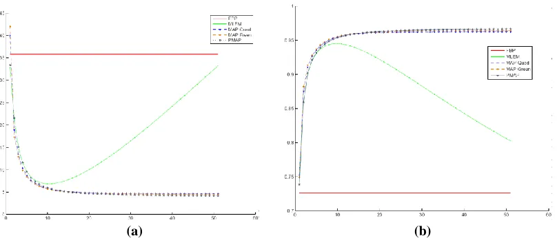
Figure5: 100K photon number observation data reconstruction error curve: (a) MSE (b) CORR From Figure 4 and figure 5 can be seen in the photon number less, serious noise pollution situation, the FBP method due to the lack of effective restraint mechanism of the noise, the reconstruction results become difficult to identify; and the image space of traditional MAP method because of constraints using only neighborhood information, the reconstruction results of noise was still obvious. In contrast, projection space MAP algorithm can provide better global constraints, and use the information of the entire image domain to correct the current pixel values, so as to obtain more smooth reconstruction results.
B. Filter Effects
In the reconstruction process, the filter L is replaced, which has different effects on the reconstruction results. In this experiment, Shepp-Logan template is still used for simulation. The different filters used are shown in figure 6. We reconstructed the 500K photon number data and the 100k photon number data respectively, and the reconstruction results are shown in Figure 7, shown in figure 8.
Figure7.Reconstruction effect of different filters under 500K photon number(a):Ram-Lak, MSE=4.42%; (b): Shepp-Logan, MSE=4.63%; (c):Blackman, MSE=5.93%; (d):Hamming, MSE=5.46%; (e):generalized ramp
with α = 0:5, MSE=5.02%; (f):generalized ramp filter with α= 1:25,MSE=4.38%
Figure8: Reconstruction effect of different filters under 100K photon number(a):Ram-Lak, MSE=4.42%; (b):Shepp-Logan, MSE=4.63%; (c):Blackman, MSE=5.93%; (d):Hamming, MSE=5.46%; (e):generalized
ramp with α = 0:5, MSE=5.02%; (f):generalized ramp filter with α= 1:25,MSE=4.38%
suppress the high-frequency component more, the reconstruction result produces an over smoothing effect. From the MSE numerical value, the reconstruction result is different from the template map.
C. Spatial Resolution
Figure. 9: Simplified heart lung template
In order to test the spatial resolution property of projective space MAP method, the local shock response of some pixels in simplified heart lung template is selected (Figure 9). In Figure 9, the U region represents the heart, and the left bright spot represents the tumor. The U region and the bright spot are surrounded by the thoracic region, and the heart, tumor, and chest pixel values are 4:5:1. For the sake of simplification, the attenuation coefficient is set to 0. The traditional MAP method uses the space invariant two times a priori. In order to ensure convergence, all iterative algorithms are iterated 100 times (also using OS, SAGE and other methods to accelerate convergence). The correlation results are shown in figure 10.
Figure10.Simplified local impact response of vertical points of heart lung template CONCLUSION
the process of constructing transcendental functions, we through the filter, simulation system of generalized inverse matrix, distance weighted on the prior model, and studied the influence of different filters on the reconstruction results of different levels of noise data. In order to obtain approximately consistent image spatial resolution, we study the local shock response of the algorithm, and modify a priori term definition accordingly. Finally, the ML estimation is used to estimate the super parameters, and an alternating iterative algorithm is designed to optimize the reconstructed image and hyper parameters simultaneously. Experimental results show that the proposed algorithm can effectively improve the quality of reconstruction in low photon number, and provide smooth reconstruction results.
REFERENCES
[1]. L. A. Shepp, Y. Vardi. Maximum likelihood reconstruction for emission tomography. IEEE Trans. Med. Imaging [J], 1982. 1(2): 113-122.
[2]. J. A. Fessler, A. O. Hero Iii. Penalized maximum-likelihood image reconstruction using space-alternating generalized EM algorithms. Image Processing, IEEE Transactions on [J], 1995. 4(10): 1417-1429.
[3]. J. A. Fessler. Penalized weighted least-squares image reconstruction for positron emission tomography. Medical Imaging, IEEE Transactions on [J], 1994. 13(2): 290-300.
[4]. C. V. Alvino, A. J. Yezzi Jr. Tomographic reconstruction of piecewise smooth images. Computer Vision and Pattern Recognition, 2004. CVPR 2004. Proceedings of the 2004 IEEE Computer Society Conference on [J]. 1. [5]. M. C. Hong, M. G. Kang, A. K. Katsaggelos. Regularized multichannel restoration approach for globally
optimal high-resolution video sequence. Proceedings of SPIE [J], 1997. 3024: 1306.
[6]. J. Kalifa, A. Laine, P. D. Esser. Regularization in tomographic reconstruction using thresholding estimators. Medical Imaging, IEEE Transactions on [J], 2003. 22(3): 351-359.
[7]. E. Levitan, G. T. Herman. A Maximum a Posteriori Probability Expectation Maximization Algorithm for Image Reconstruction in Emission Tomography. Medical Imaging, IEEE Transactions on [J], 1987. 6(3): 185-192. [8]. J. A. Fessler. Resolution properties of regularized image reconstruction methods. Ann Arbor, MI [J], 1995:
48109-2122.
[9]. J. A. Fessler, W. L. Rogers. Spatial resolution properties of penalized-likelihood image reconstruction: space-invariant tomographs. Image Processing, IEEE Transactions on [J], 1996. 5(9): 1346-1358.
[10]. J. W. Stayman, J. A. Fessler. Compensation for no uniform resolution using penalized-likelihood reconstruction in space-variant imaging systems. Medical Imaging, IEEE Transactions on [J], 2004. 23(3): 269-284.
[11]. J. W. Stayman, J. A. Fessler. Regularization for uniform spatial resolution properties in penalized-likelihood image reconstruction. Medical Imaging, IEEE Transactions on [J], 2000. 19(6): 601-615.
[12]. V. E. Johnson, W. H. Wong, X. Hu, et al. Image restoration using Gibbs priors: boundary modeling, treatment of blurring, and selection of hyper parameter. IEEE Transactions on Pattern Analysis and Machine Intelligence [J], 1991. 13(5): 413-425.
[13]. P. C. Hansen. Analysis of Discrete Ill-Posed Problems by Means of the L-Curve. SIAM Review [J], 1992. 34: 561.
[14]. J. A. Fessler, S. D. Booth. Conjugate-gradient preconditioning methods for shift-variant PET image reconstruction. Image Processing, IEEE Transactions on [J], 1999. 8(5): 688-699.
[15]. J. Qi, R. M. Leahy. Resolution and noise properties of MAP reconstruction for fully 3-DPET. Medical Imaging, IEEE Transactions on [J], 2000. 19(5): 493-506.
[16]. J. Qi, R. H. Hues man. Theoretical study of lesion detectability of MAP reconstruction using computer observers. Medical Imaging, IEEE Transactions on [J], 2001. 20(8): 815-822.
[17]. Z. Zhou, R. Leahy, E. Mumguoclu. A comparative study of using anatomical boundary in PET reconstruction [C]. 1993.