Carbon Footprint and Order Quantity in Logistics

JIEM, 2014 – 7(2): 475-490 – Online ISSN: 2013-0953 – Print ISSN: 2013-8423 http://dx.doi.org/10.3926/jiem.1031

Carbon Footprint and Order Quantity in Logistics

Zhiyong Tian, Lingyu Huo, Guicheng Shen

School of Information, Beijing Wuzi University (China)

[email protected]; [email protected]; [email protected]

Abstract:

Purpose:

Even without economic factors and government regulations, the pressure and

motivation of corporation to reduce emissions are still increasing. This is because the key

factors for corporation to reduce emissions have been corporate social responsibility and

increasing awareness of low carbon among consumers and society not economic trade-off and

stringent government regulations. So, the purpose of this paper is to provide quantity methods

for the logistics organizations with wish of voluntary reduction and social responsibility to

reduce emissions through operations adjustment.

Design/methodology/approach:

Being difference from the traditional research that takes

economic value as objective and carbon footprint as constraint or another source of economic

cost, this paper takes carbon footprint as objective directly, order quantity as decision variable.

By referring to the traditional economic order quantity model, the paper proposes logistics

carbon footprint model which takes transport and inventory into account. Then it solves the

model by calculating the values of order quantity, carbon footprint and revenue using the

method of optimization.

Originality/value:

The study takes carbon footprint as objective directly and creates the

corresponding quantity model. By comparing with the traditional economic order quantity

model, it can provide quantity methods and some meaningful insights for the logistics

organizations to reduce emissions.

Keywords:

inventory, transport, carbon footprint, order quantity

1. Introduction

one of which is carbon cost. The question is similar to Cachon’s (2013), so is the approach for treating carbon emission.

2. The Model

The activities of logistics can lead to either economic costs or carbon footprints. Carbon footprints are equal to carbon emission factor (EF) multiplied by action data (AD). EF is greenhouse gases (GHG) emissions per unit activity. It is measured by CO2 equivalent. AD is the quantity of activities releasing GHG. For economic costs, it is easier to get the accurate data of activities generally, which can be used in calculating carbon footprints. For carbon footprints, the coefficient is more difficult to obtain. Though there are some public available data, they may not be a proper match for AD. Fortunately, our purpose is not to obtain public, authoritative and accurate data of carbon, but to support making the decision of reduction. As for lack of accurate detailed data, Daganzo (2010) believes that detailed data may be harmful to making rational decision in the analysis of logistics. Caro, Charles, Tan and Rob (2011) thinks that focusing on the life-cycle assessment and carbon footprint literature avoiding double-counting is misguided, for over-allocated emission is benefit for making efficient measure to reduce emissions. Then we believe that it can achieve the research purpose of this paper only by estimating the data about carbon footprint roughly. So, the focus of this paper is not on acquiring accurate authority data.

Our study is limited to transport and inventory, which account for a large proportion of logistics either in cost or in carbon. There are two types of carbon footprint. One is direct carbon footprint, also called variable carbon footprint, due to the activities related to output directly. The other is indirect carbon footprint, also called fixed carbon footprint, due to the supporting activities being no related to output directly. The relationship between the two types of carbon footprint is similar as that of the variable and fixed costs. The notations employed in the model are as follows:

• Atf fixed activity of transport

• Ftf EF of fixed activity of transport

• Ctf cost per unit fixed activity of transport

• Atv variable activity of transport

• Ftv EF of variable activity of transport

• Ctv cost per unit variable activity of transport

• Ahf fixed activity of inventory

• Fhf EF of fixed activity of inventory

• Ahv variable activity of inventory

• Fhv EF of variable activity of inventory

• Chv cost per unit variable activity of inventory

• Q order quantity (decision variable)

• D demand per unit time (demand speed)

We adopt the conventional hypothesis of classical inventory theory, namely deterministic demand. So, order cycle is t=Q/D. For simplicity without loss of generality, we suppose linear relationship between variable activity and carbon or cost, which is commonly used in the literatures.

2.1. Transport

The carbon footprint per unit time is:

TFt(Q) = (Ftf · Atf + Ftv · Atv ·Q)/ Q

D = Ftf Atf D

Q + Ftv Atv D

The transport cost per unit time is:

TCt(Q) = (Ctf · Atf + Ctv · Atv · Q)/Q

D = Ctf Atf D

Q + Ctv Atv D

2.2. Inventory

The carbon footprint per unit time is:

TFh(Q) = (Fhf · Ahf + Fhv · Ahv · Q 2

The inventory cost per unit time is:

The total carbon footprint per unit time is:

TF(Q) = TFt(Q) + TFh(Q) = Ftf Atf D

Q + Ftv Atv D + Fhf Ahf + Fhv Ahv Q

2 (1)

The total cost per unit time is:

TC(Q) = TCt(Q)+ TCh(Q) = Ctf Atf D

Q + Ctv Atv D + Chf Ahf + Chv Ahv Q

2 (2)

3. Analysis

Equation (1) and (2) are similar to classical EOQ model in forms of expression, so is the solving method. The two objective functions are convex by Q. So, we can get the optimal solution by first order condition (FOC).

LetQ^ denote carbon optimization order quantity (COQ), Qx _{denote EOQ. Then,}

^

Q=

√

2FtfAtfD

F_hvA_hv (3)

Qx =

√

2C_tfA_tfD

C_hvA_hv (4)

3.1. The order quantity in optimal solution

Theorem 1.

(1) if Ftf F_hv>

C_tf

C_hv , then Q^ > Q

x_;

(2) if Ftf F_hv=

C_tf

C_hv , then Q^ = Q

x_;

(3) if Ftf F_hv<

C_tf

C_hv , then Q^ < Q

x_.

Proof. Comparing equation (3) and (4), we can derive Theorem 1 easily.

Theorem 1 is similar to the result of Hua et al. (2011), which is obtained in the case of carbon trade. The second item of Theorem 1 means low carbon and low cost, in which the two objectives of carbon and cost are consistent. By optimizing cost, carbon is at its optimal situation too. This ideal case is possible because carbon has positive even linear correlation with cost for many logistics activities. For example, Tian and Yang (2013) established logistics index system to measure the level of low carbon only from the perspective of energy consumption. Meanwhile, it also means that there is no chance to reduce emissions by selecting order quantity. But the other two cases are more common, which mean that there are opportunities to reduce emissions by optimizing order quantity. Then, one question appears that the one being at optimal point leads to how much the other deviates from its optimal point? That is what we will answer in the following.

3.2. The objective value in optimal solution

Substituting (3) and (4) into the objective function (1) and (2) respectively, we get:

TF(Q^ ) = Ftv Atv D + Fhf Ahf +

√

2F_tfA_tfF_hvA_hvD

TC(Qx) = Ctv Atv D + Chf Ahf +

√

2C_tfA_tfC_hvA_hvD

Next, we still continue our analysis by supposing the role is important. We get the new objective function by removing the first two items. Then,

TF_v( ^Q)=F_tfA_tfD_^

Q+FhvAhv

^ Q

2 (5)

TC_v(Qx)=C_tfA_tf D

Qx+ChvAhv Qx

2 (6)

If order quantity deviates from optimal order quantity by r times, then

TF_v(rQ)=^ 1 2(r+

1

r )TFv( ^Q) (7)

TC_v(rQx)=1 2(r+

1

r)TCv(Qx) (8)

Obviously, if and only if r=1, the objective value is minimum. Otherwise it is larger. This is the robustness of classical EOQ that is well known.

α= Q^ Qx=

√

C_hv C_tf⋅

F_tf

F_hv (9)

For the symmetry of the problem, there is theorem 2.

Theorem 2. The relationship between cost of COQ and carbon footprint of EOQ is:

TF

v(Qx)=

1 2(α+

1

α)TFv( ^Q) (10)

TC_v( ^Q)=1

2(α+ 1

Proof. From equation (7) and (8), we can derive Theorem 2 easily.

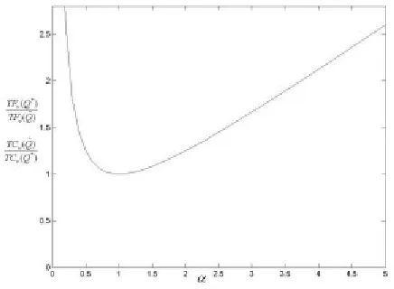
Equation (10) and (11) can be shown as Figure 1. Like classical EOQ, the objective value, either carbon or cost, shows rather robustness when order quantity changes in a certain range. E.g. when a=2, namely COQ is twice of EOQ, carbon emissions will be increased only by 25%

if choosing EOQ, and costs will be increased only by 25% if choosing COQ.

Figure 1. Ratio of objective function value and a

According to Theorem 2, if choosing COQ, the absolute amount of costs penalty is:

ΔTC=TC_v( ^Q)−TC_v(Qx)=1 2(α+

1

α−2)

√

2CtfAtfChvAhvD

If choosing EOQ, the absolute amount of carbon footprints penalty is:

ΔTF=TF_v(Qx)−TF_v( ^Q)=1 2(α+

1

α−2)

√

2FtfAtfFhvAhvD

By the two equations, it can define an economic assessment for carbon through operations adjustment, which can provide some meaningful insights for corporations in quantity. The equation is:

ΔTC

ΔTF=

√

C_tfC_hv

Theorem 2 describes the two extreme cases of order quantity, which is equal to either COQ or EOQ. It can be extended to the general case. There are some corollaries as follows.

Corollary 1. If order quantity Q is r times of COQ, then

(1) TF_v(Q)=1

2(r+ 1

r)TFv( ^Q)

(2) TC_v(Q)=1

2(rα+ 1

rα)TCv(Qx)

Proof. By substituting variables among equation (7), (8) and (9), we can derive Corollary 1 easily.

According to Corollary 1, r=1 means the decision is made by optimizing carbon, where Q is equal to COQ, and equation of corollary 1(2) is equivalent to equation (11). The case of r=1/a

means the decision is made by optimizing cost, where Q is equal to EOQ, and equation of corollary 1(1) is equivalent to equation (10).

For the symmetry of the problem, Corollary 1 can be expressed as follows.

Corollary 2. If order quantity Q is r times of EOQ, then

(1) TF_v(Q)=1₂(_αr+α_r)TF_v( ^Q)

(2) TC_v(Q)=1

2(r+ 1

r)TCv(Qx)

According to Corollary 2, r=1 means Q is equal to EOQ, and equation of Corollary 2(1) is equivalent to equation (10). The case of r=a means Q is equal to COQ, and equation of

Corollary 1(2) is equivalent to equation (11).

According to the four equations of corollary 1 and 2, when order quantity deviates from optimal order quantity, the objective value is larger than the optimal objective value. It is as follows.

TF_v(Q)

TF_v( ^Q)>1 ,

TC_v(Q)

TC_v(Qx)>1

Corollary 3. If order quantity Q is r times of COQ, then

(1) If a < 1 and r < 1

√

a , or if a > 1 and r > 1

√

a , then TF

v(Q)

TF_v( ^Q)<

TC

v(Q)

TC_v(Qx) ;

(2) If a = 1 and r = 1

√

a , then

TF_v(Q)

TF_v( ^Q)=

TC_v(Q)

TC_v(Qx) ;

(3) If a < 1 and r > 1

√

a , or if a > 1 and r < 1

√

a , then TF

v(Q)

TF_v( ^Q)>

TC

v(Q)

TC_v(Qx) .

Proof. Comparing the two equations of corollary 1, we can derive Corollary 3 easily.

Given the degree that order quantity deviates from CQO, we can judge whether the increasing of carbon footprints is larger than that of costs or not by Corollary 3. Specially, Corollary 3(1) means the effect on carbon is less than on cost, so carbon profits are larger. Corollary 3(2) means the effect on carbon is equal to on cost. Corollary 3(3) means the effect on carbon is larger than on cost, so carbon profits are smaller.

Like Corollary 1, according to equation (9), there is Corollary 4 corresponding with Corollary 3.

Corollary 4. If order quantity Q is r times of EOQ, then

(1) If a < 1 and r <

√

a, or if a > 1 and r >

√

a, then

TF_v(Q)

TF_v( ^Q)<

TC_v(Q)

TC_v(Qx) ;

(2) If a = 1 or r = a, then;

TF_v(Q)

TF

v( ^Q)

=TCv(Q)

TC_v(Qx)

(3) If a < 1 and r >

√

a, or if a > 1 and r <

√

a , then

TF_v(Q)

TF_v( ^Q)>

TC_v(Q)

TC_v(Qx) .

4. Numerical Studies

In this section we present a series of numerical examples to illustrate the above analytical results. Due to the analysis in section 3, some parameters have nothing to do with the objective. For simplicity, we only give the data of the parameters having relevant to the objective. Let D=60,000, and the rest of the parameters and the results are summarized in Table 1.

　 Ctf Chv Ftf Fhv Atf Ahv Q^ Qx a TFv TCv

Ftf Fhv

C_tf C_hv

1 36 0.3 60 0.2 5 2 232.38 146.97 1.58 92.95 88.18 300 120

2 36 0.3 60 0.2 5 2 232.38 146.97 1.58 92.95 88.18 300 120

3 40 0.4 50 0.2 5 2 212.13 134.16 1.58 84.85 107.33 250 100

4 40 0.4 50 0.2 5 2 212.13 134.16 1.58 84.85 107.33 250 100

5 40 0.2 60 0.3 5 2 189.74 189.74 1 113.84 75.89 200 200

6 40 0.4 50 0.5 5 2 134.16 134.16 1 134.16 107.33 100 100

7 50 0.4 45 0.5 5 2 127.28 150 0.85 127.28 120 90 125

8 50 0.4 45 0.5 5 2 127.28 150 0.85 127.28 120 90 125

9 60 0.4 50 0.5 5 2 134.16 164.32 0.82 134.16 131.45 100 150

10 60 0.4 50 0.5 5 2 134.16 164.32 0.82 134.16 131.45 100 150

11 60 0.4 50 0.5 5 2 134.16 164.32 0.82 134.16 131.45 100 150

12 60 0.4 50 0.5 5 2 134.16 164.32 0.82 134.16 131.45 100 150

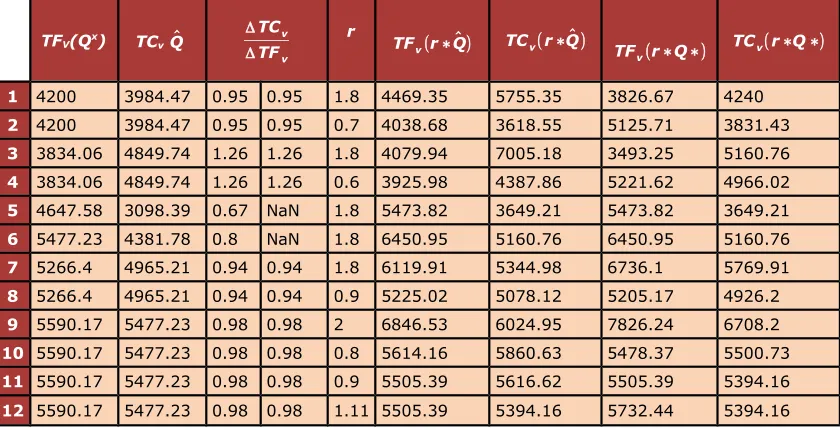
TFV(Qx) TCvQ^

ΔTC_v

ΔTF_v r TFv(r∗ ^Q) TCv(r∗ ^Q) _TF

v(r∗Q∗)

TCv(r∗Q∗)

1 4200 3984.47 0.95 0.95 1.8 4469.35 5755.35 3826.67 4240

2 4200 3984.47 0.95 0.95 0.7 4038.68 3618.55 5125.71 3831.43

3 3834.06 4849.74 1.26 1.26 1.8 4079.94 7005.18 3493.25 5160.76

4 3834.06 4849.74 1.26 1.26 0.6 3925.98 4387.86 5221.62 4966.02

5 4647.58 3098.39 0.67 NaN 1.8 5473.82 3649.21 5473.82 3649.21

6 5477.23 4381.78 0.8 NaN 1.8 6450.95 5160.76 6450.95 5160.76

7 5266.4 4965.21 0.94 0.94 1.8 6119.91 5344.98 6736.1 5769.91

8 5266.4 4965.21 0.94 0.94 0.9 5225.02 5078.12 5205.17 4926.2

9 5590.17 5477.23 0.98 0.98 2 6846.53 6024.95 7826.24 6708.2

10 5590.17 5477.23 0.98 0.98 0.8 5614.16 5860.63 5478.37 5500.73

11 5590.17 5477.23 0.98 0.98 0.9 5505.39 5616.62 5505.39 5394.16

12 5590.17 5477.23 0.98 0.98 1.11 5505.39 5394.16 5732.44 5394.16

Table 1. Results of the examples

The results in Table 1 verify Theorem 1-2 and Corollary 1-4. They show that the relationship

between EOQ (Qx_{) and COQ (Q}^ _{) was determined by the relationship between} Ftf F_hv and

the case of Ftf

F_hv ≠ C_tf

C_hv , we get Q

x_≠Q^ _{which means there are opportunities to reduce emissions}

by choosing order quantity. In the case of Ftf

F_hv =

C_tf

C_hv , the objective of cost is consistent with

the objective of carbon, and there are no opportunities to reduce emissions by operations adjustment.

If we obtain the order quantity only by one objective, such as carbon or cost, it will lead to the value of the other objective increasing. But the increasing ratio, which only depends on a, is

symmetrical for each of the two objectives. In Table 1, there are also the increasing quantities of each objective, which can act as the economic assessment standard for carbon emission. The data in Table 1 shows that the value of economic assessment standard of carbon emission does not exist when a=1, because it has already been at its optimal point for each objective.

In general, we don’t choose the order quantity by one objective only, but by the trade-off between the two objectives. In Table 1, we calculate the ratio of one objective to the other. The results verify Corollary 1-4. When we choose order quantity r times of COQ, in the case of a>1

or a<1, there exists a certain range of r. If r is within the range, the change or increasing of

carbon emissions is less than that of costs. Otherwise, the increasing of carbon emissions is larger. Only in the case of a=1 or r2=1, the changes of carbon emissions is equal to that of

costs. When choosing order quantity r times of EOQ, we can get the similar results from the data in Table 1. All these can help logistics organizations to make trade-off between costs and carbon emissions in quantity.

5. Conclusions

low carbon among consumers and society. So unlike the traditional research, we put our research in the background of corporation being social responsibility and consumers or society pursuing low carbon, and then take carbon footprint as objective directly to search out the reduction opportunities by choosing order quantity. Though we assume that corporation has the motivation to reduce emissions voluntary, economic factor is still necessary for it to survive, develop and achieve its visions. So, we also take the research on EOQ as a reference. By the comparative analysis study and a series of numerical examples, we obtained some meaningful insights. The optimal order quantity, either EOQ or COQ, has nothing to do with fixed activities of inventory and variable activities of transport. Whether EOQ is larger than COQ or not depends on the relative values of EF, cost coefficient of fixed activity of inventory and EF, cost coefficient of variable activity of transport. In extreme cases, which order quantity is equal to EOQ or COQ, the ratio of total costs and carbon footprints is rather robust. We also obtain some corollaries in general case when order quantity is not equal to EOQ or COQ. If order quantity deviates from EOQ or COQ by r times, these corollaries can be employed to judge whether the increasing ratio to the optimal value of cost is larger than that of carbon or not, which can be as the foundation for corporations to make trade-offs between cost and carbon. All these can help the corporations with social responsibility and wish of voluntary reduction to make rational decision. There are some topics for further research in this area. In this paper, we assumed that the demand is deterministic and the lead time is zero. The further research can be extended to take into account more factors influencing inventory or transport considered in the classical EOQ framework, such as stochastic demand, constant or variable lead time, discounts, and etc.

Acknowledgments

References

Arslan, M.C., & Turkay, M. (2010). EOQ Revisited with Sustainability Considerations. Working paper.

Battini, D., Persona, A., & Sgarbossa, F. (2013). A Sustainable EOQ Model: theoretical formulation and applications. International Journal of Production Economics, available online 15 August 2013.

B e a r i n g Po i n t , 4 t h S u p p l y C h a i n M o n i t o r, 2 0 1 0 - 2 0 1 1 , a v a i l a b l e o n l i n e a t

http://www.bearingpointconsulting.com/de-de/download/TAP-SC_EN.pdf (date of last access October 6th,

2013).

Benjaafar, S., Yanzhi, L., & Daskin, M. (2013). Carbon Footprint and the Management of Supply Chains: Insights From Simple Models. IEEE Transactions on Automation Science and Engineering, 10(1), 99-116. http://dx.doi.org/10.1109/TASE.2012.2203304

Blengini, G.A., & Shields, D.J. (2010). Green Labels and Sustainability Reporting. Management of Environmental Quality: An International Journal, 21(4), 477–493.

http://dx.doi.org/10.1108/14777831011049115

Bouchery, Y., Ghaffari, A., Jemai, Z., et al. (2012). Including sustainability criteria into invento r y m o d e l s . European Journal of Operational Research, 222(2), 229-240.

http://dx.doi.org/10.1016/j.ejor.2012.05.004

Cachon, G.P. (2013). Retail store density and the cost of greenhouse gas emissions. Working paper.

Carlsson, J.G., & Jia, F. (2012). Minimizing emissions in facility location. University of Minnesota working paper.

Caro, F., Charles, J.C., & Tan, T., & Rob, Z. (2011). Carbon-Option and Carbon-Neural Supply Chains. Working paper. http://dx.doi.org/10.1596/1813-9450-5878

Chen, X., Benjaafar, S., & Elomri, A. (2012). The carbon-constrained EOQ. Operations Research Letters, 41(2), 172-179. http://dx.doi.org/10.1016/j.orl.2012.12.003

Daganzo (2010). Logistics systems analysis. Beijing. Publishing house of electronics industry.

Hoen, K.M.R., Tan, T., Fransoo, J.C., et al. (2011) . Effect of carbon emission regulations on transport mode selection in supply chains. Eindhoven University of Technology.

Lieb, K.J., & Lieb, R.C. (2010). Environmental sustainability in the third-party logistics (3PL) industry. International Journal of Physical Distribution & Logistics Management, 40(7), 524-533. http://dx.doi.org/10.1108/09600031011071984

Tian, Y., & Yang, M. (2013). Demonstration analysis for the low-carbon factors index system of logistics enterprises. Journal of Industrial Engineering and Management, 6(1), 297-307.

http://dx.doi.org/10.3926/jiem.681

Wakeland, W., Sears, L., & Venkat, K. (2009). Measuring the Effects of Carbon Footprint Training on Consumers. Sustainability: The Journal of Record, 2(1), 45–52.

http://dx.doi.org/10.1089/SUS.2009.9900

Journal of Industrial Engineering and Management, 2014 (www.jiem.org)

Article's contents are provided on a Attribution-Non Commercial 3.0 Creative commons license. Readers are allowed to copy, distribute and communicate article's contents, provided the author's and Journal of Industrial Engineering and Management's names are included.