www.elsevier.com/locate/patcog
Domain described support vector classifier for
multi-classification problems
Daewon Lee, Jaewook Lee
∗Department of Industrial and Management Engineering, Pohang University of Science and Technology, Pohang, Kyungbuk 790-784, Republic of Korea
Received 8 November 2005; received in revised form 1 May 2006; accepted 6 June 2006
Abstract
In this paper, a novel classifier for multi-classification problems is proposed. The proposed classifier, based on the Bayesian optimal decision theory, tries to model the decision boundaries via the posterior probability distributions constructed from support vector domain description rather than to model them via the optimal hyperplanes constructed from two-class support vector machines. Experimental results show that the proposed method is more accurate and efficient for multi-classification problems.
䉷2006 Pattern Recognition Society. Published by Elsevier Ltd. All rights reserved.
Keywords:Multi-class classification; Kernel methods; Bayes decision theory; Density estimation; Support vector domain description
1. Introduction
Support vector machines (SVMs), originally formulated for two-class classification problems, have been successfully applied to diverse pattern recognition problems and have become in a very short period of time the standard state-of-the-art tool. The SVMs, based on the structured risk minimization(SRM), are primarily devised in order to min-imize the upper bound of the expected error by optimizing the trade-off between the empirical risk and the model com-plexity[1–3]. To achieve this, they construct an optimal hy-perplane to separatebinary classdata so that the margin is maximal.
Since many real-world applications are multi-class clas-sification problems, several approaches to extend two-class SVMs to a multi-class SVM for multi-category classifica-tions have been proposed. Most of the previous approaches try to decompose a multi-class problem to a set of multiple binary classification problems where two-class SVMs can be trained and applied. For example, one-against-all algo-rithm transforms ac-class problem intoctwo-class problems
∗Corresponding author. Tel.: +82 54 279 2209. E-mail addresses:[email protected](D. Lee), [email protected](J. Lee).
0031-3203/$30.00䉷2006 Pattern Recognition Society. Published by Elsevier Ltd. All rights reserved. doi:10.1016/j.patcog.2006.06.008
where one class is separated from the remaining ones; one-against-one (pair-wise) algorithm converts the c-class problem intoc(c−1)/2 two-class problems where pairwise optimal hyperplanes for each pair of classes are constructed and max-voting strategy is used to predict their classes, and so on (cf. [4,5]). These approaches, however, have some drawbacks inherent in the architecture of multiple binary classifications: some unclassifiable regions may exist if a data point belongs to more than one class or to none, result-ing in low accuracy in correct classification. Also, to train two-class SVMs multiple times for the same data set re-peatedly often results in a highly intensive time complexity for large scale problems.
To overcome such drawbacks, in this paper, we propose a novel support vector classifier for multi-classification prob-lems. The proposed classifier, based on the Bayesian opti-mal decision theory, tries to model the posterior probability distributions via support vector domain description (SVDD) [6,7]rather than to model the decision boundaries by con-structing optimal hyperplanes. The performance of the pro-posed method is confirmed through simulation.
with an illustrative example and Section 4 provides the the-oretical basis of the proposed method. In Section 5, simula-tion results are given to illustrate the effectiveness and the efficiency of the proposed method.
2. Previous works
In this section, we first review the Bayesian optimal de-cision theory and describe the existing density estimation algorithms. Then we briefly outline the SVDD algorithm employed in our proposed method.
2.1. Bayesian optimal decision theory
According to the Bayesian decision theory, an optimal classifier can be designed if we know the prior probabil-ities p(wi) and the class-conditional densities p(x|wi),
that is, with Bayes formula, the posterior probabilities are given by
p(wi|x)=
p(x|wi)p(wi)
p(x)
=p(x|wi)p(wi) c
i=1p(x|wi)p(wi)
, (1)
wherecis the number of output class labels. The optimal decision rule to minimize the average probability of error can then be shown to be the Bayesian decision rule[8,9]that selects thewi maximizing the posterior probabilityp(wi|x)
as follows:
Decidewi ifp(wi|x) > p(wj|x) for allj =i. (2)
In typical classification problems, estimation of the prior probabilities presents no serious difficulties (normally all are assumed to be equal or Ni/N). However, estimation
of the class-conditional densities is quite another matter. During the last decades, lots of density estimation algo-rithms have been proposed and the existing density esti-mation algorithms may generally be categorized into three approaches: parametric, semi-parametric, and nonparametric methods.
Parametric methods assume a specific functional form of
p(x|wi)to contain a number of adjustable parameters. The
simplest and the most widely used form is a normal distri-bution given by
p(x|wi,i,i)=
1
(2)(d/2)|i|1/2
exp
−1
2(x−i) T−1
i (x−i)
. (3)
The drawback of such an approach is that a particular form of parametric function might be incapable of describing the true data distribution.
Second, semi-parametric methods have a form of finite mixtures of Gaussians as follows:
p(x|wi,1, . . . ,M)=
M
k=1
p(x|wi,k, k)p(k), (4)
where p(x|wi,k, k) is a kth component in the form of
Gaussian function andp(k)are mixing parameters. In semi-parametric methods, training data do not provide any
com-ponent labels to say which component was responsible for
generating each data point. To select the number of compo-nents and to estimate its parameters, however, we need to in-corporate with an iterative scheme such as an EM algorithm, which often proved to be highly computationally extensive. The third approach is nonparametric methods which es-timate the class-conditional density function as a weighted sum of a set of kernel functions, K(·,·), to be determined entirely by the data
p(x|wi)= N
j=1
jK(xj,x). (5)
Though such methods have the most descriptive capability, they typically suffer from the problem that the number of parameters grows with the size of the data set, so that the models can quickly become unwieldy.
2.2. Support vector domain description
The existing methods for density estimation have a trade-off between a descriptive ability and a computational burden. To solve this problem, our proposed method utilizes a so-called trained kernel support function that characterizes the support of a high dimensional distribution of a given data set, inspired by the SVMs. We first review a support vector domain description (SVDD) procedure (also called a one-class support vector machine). Then we build a trained kernel support function, to be used as a pseudo-density function, via SVDD.
The basic idea of SVDD is to map data points by means of a nonlinear transformation to a high dimensional feature space and to find the smallest sphere that contains most of the mapped data points in the feature space [6,7]. This sphere, when mapped back to the data space, can separate into several components, each enclosing a separate cluster of points. More specifically, let{xi} ⊂Xbe a given training data set of X ⊂ Rn, the data space. Using a nonlinear transformationfromXto some high dimensional feature space, we look for the smallest enclosing sphere of radius
Rdescribed by the following model:
min R2+C
j
j
s.t. (xj)−a2R2+j,
wherea is the center and j are slack variables allowing for soft boundaries. To solve this problem, we introduce the Lagrangian
L=R2−
j
(R2+j− (xj)−a2)j
−
j
jj+C
j
j.
Setting jL/jR =0 andjL/ja=0, respectively, leads to
jj=1 and
a=
j
j(xj). (7)
Using these relations and transforming the objective function into a function of the variablesj only, the solution of the primal (6) can then be obtained by solving the following Wolfe dual problem:
max W=
j
K(xj,xj)j −
i,j
ijK(xi,xj)
s.t. 0jC,
j
j=1, j=1, . . . , N, (8)
where the Gaussian kernel K(xi,xj)=(xi)·(xj)=
exp(−qxi −xj2)with width parameterq is used. Only those points with 0<j< C lie on the boundary of the sphere and are called support vectors (SVs). The trained Gaussian kernel support function, defined by the squared ra-dial distance of the image of x from the sphere center, is then given by
f (x):=R2(x)= (x)−a2
=K(x,x)−2
j
jK(xj,x)
+
i,j
ijK(xi,xj) (9)
and the domain that describes the support of the data points is given by {x : f (x)= ˆR2} whereRˆ2=R2(xi) for any
support vectorxi.
3. The proposed method
In this section, we present a method for multi-classification problems. Suppose that a set of training data {(xi, yi)}Ni=1 ⊂ X×Y is given where xi ∈ X denotes
an input pattern and yi ∈ Y= {w1, . . . , wc} denotes its output class. The central idea of the proposed method is to utilize the information of the domain description gen-erated by the SVDD for estimating the distributions of each partitioned class data and then to utilize the esti-mates to classify a data point via Bayesian decision rule. The detailed procedure of the proposed method is as follows:
Step 1 (Data partitioning): We first partition the given training data into c-disjoint subsets {Dk}ck=1 according to their output classes. For example, thekth class data set,Dk, containsNk elements as follows:
Dk= {(xi1, wk), . . . , (xiNk, wk)}. (10)
Step 2 (SVDD for each class data set): For each class data set Dk, we build a trained Gaussian kernel support function via SVDD. Specifically, we solve the dual problem Eq. (8). Let its solution be ¯il, l=1, . . . , Nk, and Jk ⊂
{1, . . . , Nk}be the set of the index of the nonzero¯il. The
trained Gaussian kernel support function for each class data setDk is then given by
fk(x)=1−2
il∈Jk
¯
ile−qNx−xil2
+
il,im∈Jk
¯
il¯ime−qNxil−xim2. (11)
Step3 (Constructing a pseudo-density function for each class): We construct the following pseudo-density function for each classk=1, . . . , c:
ˆ
p(x|wk)=12(rk−fk(x)) for k=1, . . . , c, (12) whererk=R2(xsk)for any support vector xsk offk(·).
Step 4 (Classification using estimated pseudo-posterior probabilities): For each class k, k = 1, . . . , c, we esti-mate a pseudo-posterior probability distribution function as follows:
(wk|x)=const.× ˆp(wk|x)= ˆp(wk)· ˆp(x|wk)
=Nk
N (−fk(x)+rk), (13)
wherep(ˆ x|wi)is a pseudo-density function obtained in step
2. Then we classifyxinto the class
arg max
k=1,...,c(wk|x).
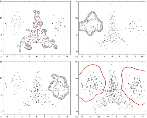
To illustrate the proposed method, seeFig. 1where a data set with three classes is given. At step 1, we partition the given data set into three data sets according to their output classes and perform the SVDD for each class-conditional data set at step 2. At step 3, using the trained Gaussian kernel support functions obtained in step 2, we construct the pseudo-density functions given by Eq. (12) for each classi=1,2,3 which are shown in (a)–(c) ofFig. 1. At step 4, we determine the final decision boundary via posterior density estimates in Eq. (13), which is shown in (d) ofFig. 1.
The constructedpseudo-density function in Eq. (12) has several nice properties compared with the existing methods reviewed in Section 2. Firstly, each p(ˆ x|wk)(up to a
15
10
5
0
15
10
5
0
15
10
5
0
15
10
5
0
-2 0 2 4 6 8 10 12 14 -2 0 2 4 6 8 10 12 14
-2 0 2 4 6 8 10 12 14 -2 0 24 6 8 10 12 14
(a) (b)
(d) (c)
Fig. 1. Illustration of the proposed method applied to thetriangledata set. (a), (b), and (c) denote contours of pseudo-density functions on classes 1, 2, and 3, respectively. In (d), a red solid line represents a final decision boundary determined by the estimated posterior-density functions.
Theorem 1 in Section 4. Secondly, since only a small portion of the ¯j turn out to have nonzero values (corresponding points are SVs) as a result of optimizing Eq. (8), the con-structed estimate highly reduces the computational burden involved in the computation ofp(ˆ x|wk). Finally, as shown
in Theorem 2 in Section 4, for a finite sample size, each set {x:p(ˆ x|wk)0}estimates a support of its class-conditional
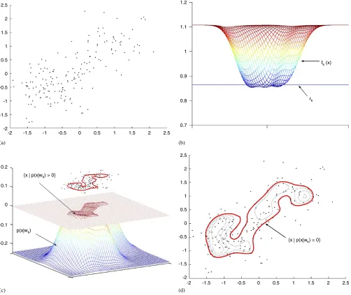
distribution and has a good enough descriptive ability to de-scribe highly nonlinear and arbitrary-shaped structures, in-cluding multi-modal or noisy distributions (seeFig. 2).
4. Theoretical basis
In this section we provide a theoretical basis for the proposed method developed in the previous section. To be-gin with, we give an asymptotic convergence result for the
constructed pseudo-density functions in our proposed method to estimate the unknown class-conditional densities for large sample size. Then we present a theoretical result on the generalization error, which characterizes estimation er-ror of the support of the data distribution for a finite sample size.
Theorem 1. Let N samples x1, . . . , xN ∈ Rd be drawn
independently and identically distributed(i.i.d.) according
to some unknown probability law p(x) and the estimate
pN(x)is given by
pN(x)=(qN/)d/2 N
i=1
ie−qNx−xi2,
where the i are the set of the coefficients satisfying
N
2.5
2.5 2
2 1.5
1.5 1
1 0.5
0.5 0
0 -0.5
-0.5 -1
-1 -1.5
-1.5 -2
-2
1.2
1.1
1
0.9
0.8
0.7
fk (x)
rk
0.2
0.1
0
-0.1
-0.2
{x | p(x|wk) > 0}
{x | p(x|wk) = 0}
p(x|wk)
2.5
2.5 2
2 1.5
1.5 1
1 0.5
0.5 0
0 -0.5
-0.5 -1
-1 -1.5
-1.5 -2
-2
(a) (b)
(c) (d)
Fig. 2. Illustrations of steps 2 and 3 of the proposed method: (a) is akth class data artificially generated from the mixture of three 2D Gaussian functions; (b) is a trained Gaussian kernel support functionfk(x)obtained in step 2; (c) presents apseudo-density functionp(ˆ x|wk)in Eq. (12) obtained in step 3; (d) shows a contour plot of{x| ˆp(x|wk) >0}where the region inside the solid line represents an estimate of the support of its class distribution.
CN, qNsatisfy the following conditions:
lim
N→∞qN= ∞ and Nlim→∞CNq d/2
N =0.
Then the estimatepN(x)converges top(x), i.e.,
lim
N→∞p¯N(x)=p(x),
lim
N→∞¯
2
N(x)=0.
Proof. Let
N(x−xi)=(qN/)d/2e−qNx−xi
2 .
Then we haveN(x−xi)dx=1 andN(x−xi)approaches
a Dirac delta function centered at xi as qN approaches to
infinity. From this fact, we get
¯
pN(x)=E[pN(x)] = N
i=1
iE[(qN/)d/2e−qNx−xi
2 ]
=
N
i=1
i N(x−v)p(v)dv
−→
(x−v)p(v)dv=p(x) asN → ∞
since Ni=1i =1 and qN → ∞ as N → ∞. Because
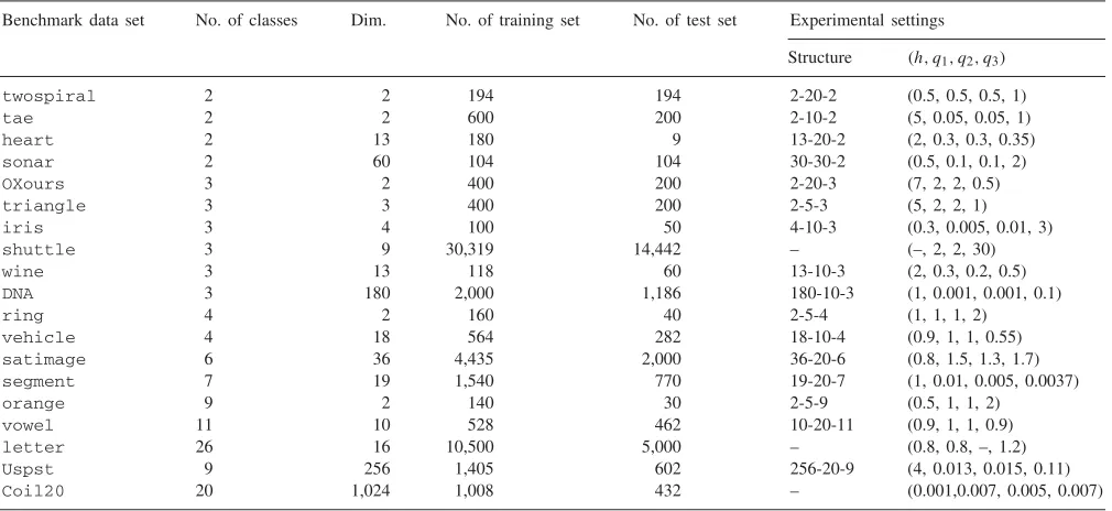
Table 1
Benchmark data description and experimental settings
Benchmark data set No. of classes Dim. No. of training set No. of test set Experimental settings Structure (h, q1, q2, q3)
twospiral 2 2 194 194 2-20-2 (0.5, 0.5, 0.5, 1)
tae 2 2 600 200 2-10-2 (5, 0.05, 0.05, 1)
heart 2 13 180 9 13-20-2 (2, 0.3, 0.3, 0.35) sonar 2 60 104 104 30-30-2 (0.5, 0.1, 0.1, 2) OXours 3 2 400 200 2-20-3 (7, 2, 2, 0.5) triangle 3 3 400 200 2-5-3 (5, 2, 2, 1)
iris 3 4 100 50 4-10-3 (0.3, 0.005, 0.01, 3)
shuttle 3 9 30,319 14,442 – (–, 2, 2, 30)
wine 3 13 118 60 13-10-3 (2, 0.3, 0.2, 0.5)
DNA 3 180 2,000 1,186 180-10-3 (1, 0.001, 0.001, 0.1)
ring 4 2 160 40 2-5-4 (1, 1, 1, 2)
vehicle 4 18 564 282 18-10-4 (0.9, 1, 1, 0.55) satimage 6 36 4,435 2,000 36-20-6 (0.8, 1.5, 1.3, 1.7) segment 7 19 1,540 770 19-20-7 (1, 0.01, 0.005, 0.0037) orange 9 2 140 30 2-5-9 (0.5, 1, 1, 2)
vowel 11 10 528 462 10-20-11 (0.9, 1, 1, 0.9) letter 26 16 10,500 5,000 – (0.8, 0.8, –, 1.2) Uspst 9 256 1,405 602 256-20-9 (4, 0.013, 0.015, 0.11) Coil20 20 1,024 1,008 432 – (0.001,0.007, 0.005, 0.007) In theexperimental settingscolumn, structure means network structure ofBR-NNandhis a window size ofBDM-Parzen.q1, q2, q3are the Gaussian kernel parameters of1-1-SVM,1-all-SVM, andProposedmethod, respectively.
random variables, its variance is the sum of the variances of the separate terms, and hence
¯2
N(x)
=
N
i=1
E i(qN/)d/2e−qNx−xi
2 − 1
Np¯N(x) 2
=N
i=1
E[2i(qN/)de−2qNx−xi
2 ] − 1
Np¯N(x)
2
max
i i
(qN/)d/2E
× N
i=1
i(qN/)d/2e−qNx−xi
2 ·1
− 1
Np¯N(x)
2
CN(qN/)d/2E[pN(x)] =CNqNd/2−d/
2¯
pN(x)
→0 asN → ∞
since maxiiCN andCNqNd/2asN → ∞.
Since the dual optimal solutions ¯j where (C, q) = (CN, qN) are in the set SN = { = (1, . . . ,N)T :
N
i=1i =1, 0iCN}and the volume of the set SN
shrinks to zero as CN → ∞, controlling the parameters
(CN, qN)as above leads to the second term of the trained
Gaussian kernel support function f converging to an un-known density function up to a constant multiple.
In relation with our pseudo-density function constructed via the SVDD, note that for eachk,k=1, . . . , c, Eq. (12) can be written as
ˆ
p(x|wk)=
⎛ ⎝
il∈Jk
¯
ile−qNx−xil2−
il∈Jk
¯
ile−qNxsk−xil2 ⎞ ⎠.
(14)
Since the second term of the right-hand side converges to zero as qN → ∞, each p(ˆ x|wk)(up to a constant
multi-ple) plays the role of an asymptotic estimate for a class-conditional density function.
We next present a result on generalization error bound, which explains theoretically how the constructed pseudo-density function characterizes the support of the class-conditional distributions.
Theorem 2. Let N samplesx1, . . . , xN be drawn
indepen-dently and identically distributed(i.i.d.)according to some
unknown probability distribution law P,which does not
con-tain discrete components. Suppose,moreover,we solve the
optimization problem Eq.(6) and obtain a solution f given
explicitly by Eq. (9).LetCa,r := {x :f (x)r}denote the
induced region for a level value r.With probability1−
over the draw of the random sample x1, . . . , xN, for any
>0,
P{x:x∈/Ca,Rˆ2+} 2
N
k+log2
N2
2
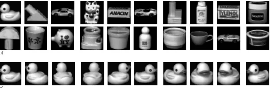
Fig. 3. (a) Images of 20 different objects in theCoil20data set. (b) Different poses from different angles of the first object (in the same class) in the Coil20data set.
where
k=c1log(c2ˆ
2
N)
ˆ
2 +Dˆlog2
e
(2N−1)ˆ
D +1
+2,
c1=16c2, c2=ln(2)/(4c2), c=103, ˆ
=/a, D=
i
max{0, f (xi)− ˆR2},
andRˆ2=R2(xs)for any support vector xs off (·).
Proof. Consider the problem of returning a function that takes the value+1 in a small region capturing most of the data points and−1 elsewhere. Mapping the data into the fea-ture space corresponding to the kernel and separating them from the origin with maximum margin can be formulated as the following quadratic programming (QP).
min 1
2w 2+
C
j
j−
s.t. (w·(xj))−j, j0. (15)
Then the functiongiven by
(x)=w·(x)=
j
jK(xj, x), (16)
w=
j
j(x), (17)
where the j are the solution of the Wolfe dual form of problem Eq. (15):
min W=1
2
i,j
ijK(xi,xj)
s.t. 0jC,
j
j=1, j=1, . . . , N, (18)
describes the decision function that solves problem Eq. (15) by choosing the sign of((x)− ˆ)whereˆ=(xi)for any
support vectorxi. For a Gaussian kernel whereK(x,x)=1, problem Eq. (18) is equivalent to problem Eq. (8). Therefore, we have
w=a,
f (x):=R2(x)=1−2(x)+ a2.
Therefore, the generalization error bound in[10, Theorem 1] can be equally applied to get the result by changing
w −→ a = w, −→ ˆR2=1−2+ a2,
−→=2,
D=
i
max{0,ˆ−(xi)} −→D
=
i
max{0, f (xi)− ˆR2} =2D.
5. Simulation results
To demonstrate the performance of the proposed method empirically, we have conducted simulations on some clas-sification problems which are categorized as follows. And additional description of the data sets is given inTable 1.
Artificial data:twospiral,tae,OXours,triangle, ring, and orangeare generated from highly nonlinear-shaped distribution in order to demonstrate generalization capability of the various methods.
Small-scale real-world data: heart, sonar, iris, wine,vehicle,vowelare from the UCI machine learn-ing repository[11]and Statlog database[12].
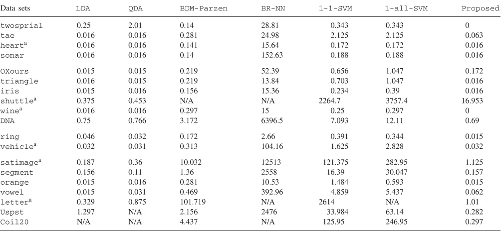
Table 3
Simulation results on benchmark problems: model building time (s)
Data sets LDA QDA BDM-Parzen BR-NN 1-1-SVM 1-all-SVM Proposed
twosprial 0.25 2.01 0.14 28.81 0.343 0.343 0
tae 0.016 0.016 0.281 24.98 2.125 2.125 0.063
hearta 0.016 0.016 0.141 15.64 0.172 0.172 0.016 sonar 0.016 0.016 0.14 152.63 0.188 0.188 0.016 OXours 0.015 0.015 0.219 52.39 0.656 1.047 0.172 triangle 0.016 0.015 0.219 13.84 0.703 1.047 0.016
iris 0.015 0.016 0.156 15.36 0.234 0.39 0.016
shuttlea 0.375 0.453 N/A N/A 2264.7 3757.4 16.953
winea 0.016 0.016 0.297 15 0.25 0.297 0
DNA 0.75 0.766 3.172 6396.5 7.093 12.11 0.69
ring 0.046 0.032 0.172 2.66 0.391 0.344 0.015
vehiclea 0.032 0.031 0.313 104.16 1.625 2.828 0.032 satimagea 0.187 0.36 10.032 12513 121.375 282.95 1.125 segment 0.156 0.11 1.36 2558 16.39 30.047 0.157 orange 0.015 0.016 0.281 10.53 1.484 0.593 0.015 vowel 0.015 0.031 0.469 392.96 4.859 5.437 0.062 lettera 0.329 0.875 101.719 N/A 2614 N/A 1.01 Uspst 1.297 N/A 2.156 2476 33.984 63.14 0.282 Coil20 N/A N/A 4.437 N/A 125.95 246.95 0.297
aThe corresponding data set is normalized and N/A meansnot available.
(image segmentation data), letter (classification of the English alphabet images) [12], Uspst (handwritten digit recognition), Coil20(classification of gray-scale images of 20 objects, seeFig. 3)[13].
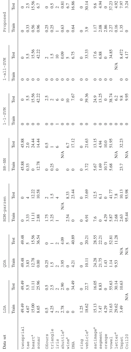
The performance of the proposed method is compared with six widely used methods; linear discriminant analysis (LDA), quadratic discriminant analysis (QDA), Bayesian decision method using parzen windows (BDM-parzen), Bayesian regularization neural network (BR-NN), one-against-one SVM (1-1-SVM), and one-against-all SVM (1-all-SVM)[5]. The criteria for evaluating the performance of these methods are their mis-classification error rates for training data sets and test data sets (Table 2), and model building time (Table3).
We chose the best parameters by performing model se-lection. That is, alternative models are constructed on the training data where the test data are assumed unknown and then the parameter set, with the best performance for the test set, is selected for constructing the final model. In our experiments, to reduce the search space of parameter sets, we used the same q values in all the pseudo-density functions of Eq. (12) (by settingC=1, i.e., not using soft margins). The detailed descriptions of parameter values are reported in the last column ofTable 1. Also the struc-ture inTable 1 means a network architecture of BR-NN. For example, 13-20-2 means a multi-layer neural network architecture that has an input layer with 13 nodes, a hid-den layer with 20 nodes, and an output layer with two nodes.
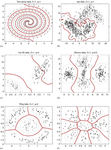
Experimental results are shown in Fig. 4,Tables 2, and 3. Fig. 4shows a decision boundaries, constructed by the
proposed method applied to multi-class data sets (from 2 class to 9 class problems) including highly nonlinear shaped data sets (e.g., two-spiral data). In Tables 2 and 3, train,
test, andtimedenote training error (%), test error (%), and computation time for model building (s), respectively. Ex-perimental results demonstrate that the proposed method achieves a better or comparable performance in terms of ac-curacy and efficiency for most of the multi-class data sets (even for two-class data sets).
To analyze the time complexity of the proposed method and conventional SVM methods, let N be the number of training pattern andcis the number of output class labels. Both the proposed method and the conventional SVM have a QP procedure and most of the QP solvers have time complexityO(N3)[14], so that the computational load for the large-scale multi-class problems is quite intensive (for example, in Table 2, 1-all-SVM on letter data is not available due to lack of memory). Generally, the SVM ap-proaches for multi-classification adopt one of one-against-one or one-against-all. The one-against-one SVM for multi-classification decomposes the multi-class problems into(c·(c−1))/2 binary subproblems, each one composed of (2N)/c. Its time complexity, therefore, is O((4N3)/c). The one-against-allSVM uses cdifferent SVMs and each one has N training patterns, so that its time complexity is
O(c·N3). The proposed method uses c QP problems of Eq. (8) and each one has N/c training patterns. There-fore, the time complexity of the proposed method is
6
6 4
4 2
2 0
0 -2
-2 -4
-4
6
4 8 10 12 14
2 0 -2 -4 -6
11
10
9
8
7
6
5
-3 -2.5 -2 -1.5 -1
-2 -1 0 1 2
-0.5 0 0.5 1 1.5
-2 -2
-1.5 -1.5
-1 -1
-0.5 -0.5
0 0
0.5 0.5
1 1
1.5 1.5
2 2.5
-2 -1.5 -1 -0.5 0 0.5 1 1.5 2 2.5
2 -6
15
15 20
10
10 5
5 0
0 -5
-5 -10
-10
8
6
4
2
0
-2 10
Two-spiral data, C=1, q=1 tae data, C=1, q=1
Iris 2D data, C=1, q=4 OXours data, C=1, q=0.5
Ring data, C=1, q=2
(a) (b)
(c) (d)
(f) (e)
Fig. 4. Experimental results on the 2D benchmark data sets where the red solid lines represent decision boundaries.
6. Conclusions
In this paper, a new classifier for multi-class classification problems has been proposed. The proposed method utilizes the information of the domain description generated by the SVDD to estimate the distributions of each partitioned class data. Then it classifies a data point with this estimate ac-cording to the Bayesian decision rule. Benchmark results demonstrate that the proposed method is more accurate, ef-ficient, and robust compared to other existing methods. The application of the method to more diverse real-world prob-lems remains to be investigated.
Acknowledgment
This work was supported partially by the Korea Re-search Foundation under the Grant number KRF-2005-041-D00708 and partially by the KOSEF under the Grant number R01-2005-000-10746-0.
References
[2]V.N. Vapnik, An overview of statistical learning theory, IEEE Trans. Neural Networks 10 (1999) 988–999.
[3]K.-R. Muller, S. Mika, G. Rätsch, K. Tsuda, B. Schölkpf, An introduction to kernel-based learning algorithms, IEEE Trans. Neural Networks 12 (2) (2001) 181–202.
[4]C.-W. Hsu, C.-J. Lin, A comparison of methods for multiclass support vector machines, IEEE Trans. Neural Networks 13 (2002) 415–425. [5]J. Weston, C. Watkins, Multi-class support vector machines, in: M. Verleysen (Ed.), Proceedings of ESANN99, Brussels, Belgium, 1999. [6]D.M.J. Tax, R.P.W. Duin, Support vector domain description, Pattern
Recogn Lett. 20 (1999) 1191–1199.
[7]J. Lee, D. Lee, An improved cluster labeling method for support vector clustering, IEEE Trans. Pattern Anal. Mach. Intell. 27 (3) (2005) 461–464.
[8]C.M. Bishop, Neural Networks for Pattern Recognition, Oxford University Press, Oxford, 1995.
[9]R.O. Duda, P.E. Hart, D.G. Stork, Pattern Classification, Wiley-Interscience Publication, New York, 2001.
[10]B. Schölkpf, J.C. Platt, J. Shawe-Taylor, A.J. Smola, Estimating the support of a high-dimensional distributions, Neural Comput. 13 (2001) 1443–1471.
[11] http://www.ics.uci.edu/∼mlearn/MLRepository.html, UCI Reposi-tory of machine learning databases.
[12]D. Michie, D.J. Spiegelhalter, C.C. Taylor, Machine Learning, Neural and Statistical Classification, Ellis Horwood, Chichester, UK, 1994. [13]O. Chapelle, A. Zien, Semi-supervised classification by low density separation, Proceedings of the Tenth International Workshop on Artificial Intelligence and Statistics, 2005, pp. 57–64.
[14]J.C. Platt, Fast training of support vector machines using sequential minimal optimization, Advances in Kernel Methods: Support Vector Machines, MIT Press, Cambridge, MA, 1999, pp. 185–208.
About the Author—DAEWON LEE received B.S. in industrial engineering from Pohang University of Science and Technology (POSTECH) in 2002 and is currently a Ph.D. candidate in the Department of Industrial and Management Engineering at POSTECH. He is interested in pattern recognition, support vector machine, and their applications to data mining.
About the Author—JAEWOOK LEE is an associate professor in the Department of Industrial and Management Engineering at Pohang University of Science and Technology (POSTECH), Pohang, Korea. He received the B.S. degree from Seoul National University, and the Ph.D. degree from Cornell University in 1993 and 1999, respectively.