Accounting for Changes in Between-Group Inequality
Ariel Burstein Eduardo Morales Jonathan Vogel
UCLA Princeton University Columbia University
Determinants of Changes in Relative Demand
Pronounced changes in between-group inequality in U.S., e.g., more educated workers relative to less educated workers women relative to men
=⇒large changes in relative demand
Voluminous literature—following Katz and Murphy (1992)—studying how changes in relative supply and demand for labor groups shape relative wages Changes in relative demand have been linked to, e.g.,
computerization (or a reduction in price of equipment more generally)
e.g., Krusell et al. (00), Acemoglu (02), Autor and Dorn (13), Beaudry and Lewis (14)
changes in relative productivity or demand across occupations or sectors (driven by structural transformation, offshoring, international trade...)
e.g., Autor et al. (03), Grossman and Rossi-Hansberg (08), Buera et al. (15)
Computerization
1984 1989 1993 1997 2003
All 27.4 40.1 49.8 53.3 57.8
Education College 45.5 62.5 73.4 79.8 85.7
Non-college 22.1 32.7 41.0 43.7 45.3
Gender Female 32.8 47.6 57.3 61.3 65.1
Male 23.6 34.5 43.9 47.0 52.1
Computer use rises over time
Changes across occupations
−1
−.5
0
.5
1
Growth of occupation labor payment share
0 .2 .4 .6 .8 1
Occupation college intensity averaged over 1984 & 2003
−1
−.5
0
.5
1
Growth of occupation labor payment share
0 .2 .4 .6 .8 1
Occupation female intensity averaged over 1984 & 2003
Decomposing Changes in Relative Wages
Assignment framework building on Eaton and Kortum (2002), Hsieh et al. (2013), and Lagakos and Waugh (2013)
many groups of workers (in empirics: 30 education-gender-age groups) many occupations (in empirics: 30 e.g. executives, technicians )
extended to incorporate equipment (in empirics: computers vs. other)
Changes in relative wages across worker groups are shaped by shocks to labor composition (relative supply of labor groups)
occupation shifters(combo of changes in demand and productivity of occs) equipment productivity(combo of changes in cost/productivity of equipment) labor productivity(combo of factors affecting productivity of worker groups, independent of equipment and occupations)
Comparative Advantage
Impact of shocks on inequality shaped by comparative advantage Consider impact of computerization
A labor group may use computers intensively for two reasons has direct comparative advantage (CA) with computers
uses computers relatively more within an occupation computerization increases wages of these worker groups this is the case for more educated workers
has direct CA in occupations in which computers also have direct CA uses computers as intensively as any other labor group within an occupation computerization may increase or decrease wages of these worker groups this is the case for female workers
Measuring comparative advantage btw worker groups, equipment types, occupations a key ingredient in quantitative analysis
Preview of the Results: 1984-2003
Using data on
allocations of workers to equipment types and occupations, and wages,
decompose changes in between-group inequality
Computerization⇒majority of rise in between-education-group inequality at
high and low levels of education aggregation (∼60% for skill premium)
Occupation shifters and computerization⇒ ∼80% of rise in skill premium
Contrasts with most previous results attributing rise in skill premium largely to unobservables; e.g. Bound et al. (1992) and Lee and Wolpin (2010)
Relation to a large literature
Approach: A simple assignment (Ricardo-Roy) model...
Assumptions build on Eaton and Kortum (2002), previously applied to labor markets by Hsieh et al. (2013) and Lagakos and Waugh (2013)
... extended to incorporate equipment
Objective: Link quantitative evolution of inequality to observables Most similar to Krusell et al. (2000) Lee and Wolpin (2010) Our approach allows for greater disaggregation using detailed factor allocations (allocation of workers to occupations and computer use)
Related work using differential regional exposure to computerization studies differential effect across regionsAutor and Dorn (2013), Beaudry and Lewis (2014) Complement by embedding computerization into GE model to quantify effect of computerization (+ other shocks) on evolution of inequality
Rely on detailed data on computer usage across workers rather than regional variation in exposure
Relation to a large literature
Approach: A simple assignment (Ricardo-Roy) model...
Assumptions build on Eaton and Kortum (2002), previously applied to labor markets by Hsieh et al. (2013) and Lagakos and Waugh (2013)
... extended to incorporate equipment
Objective: Link quantitative evolution of inequality to observables Most similar to Krusell et al. (2000) Lee and Wolpin (2010) Our approach allows for greater disaggregation using detailed factor allocations (allocation of workers to occupations and computer use)
Related work using differential regional exposure to computerization studies differential effect across regionsAutor and Dorn (2013), Beaudry and Lewis (2014) Complement by embedding computerization into GE model to quantify effect of computerization (+ other shocks) on evolution of inequality
Rely on detailed data on computer usage across workers rather than regional variation in exposure
Outline
Model
Without sectors and without international trade Equilibrium in changes
Intuition
Decomposing Changes in Relative Wages Describing the data
Factor allocation and comparative advantage
Measuring changes in equipment and occupation shifters Estimation of parameters
Environment
Static environment with a unique final good Economy is closed
All markets are competitive
CES technology mapping the services from occupations to the final good
Yt =
X
ω µt(ω)
1
ρYt(ω) ρ−1
ρ ρρ−1
, ρ >0
The final good may be used for consumption or to produce equipment goods
Ct+
X
κ
Occupation Production Function
There is a continuum of workersz ∈ Zt who supply labor inelastically
All workers have an identical homothetic utility function increasing inCt
Workers are divided into labor groups, indexed byλ
The output of a workerz∈ Zt(λ) who useskt units of equipmentκin the
production of occupationω is
[Tt(λ, κ, ω)εt(z, κ, ω)]1−αkt(κ)α
with
εt(z, κ, ω)∼Fr´echet : G(ε) = exp(−ε−θ), θ >1
In paper we incorporate absolute advantage withinλ
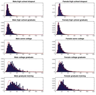
Fr´echet analytically tractable and provides reasonable approximation of observed wage distribution; e.g., Saez (2001) and figures below
Occupation Production Function
[Tt(λ, κ, ω)εt(z, κ, ω)]1−αkt(κ)α
Cobb-Douglas production function at the level of occupation Whenρ >1, employment grows in computer-intensive occupations
Even though strong restrictions are imposed on the occupation production function, aggregate implications for wages nest those of
canonical model; e.g. Katz and Murphy (1992)
Partial Equilibrium
Given price of each occupation,pt(ω), and price of each type of equipment,
pt(κ), each workerz ∈ Zt(λ) chooses
a type of equipmentκand an occupationω; and, given the choice (κ, ω), the quantity of equipmentk
The probability that a workerz ∈ Zt(λ) chooses the pair (κ, ω) is
πt(λ, κ, ω) =
h pt(κ)
−α
1−αpt(ω)
1
1−αTt(λ, κ, ω) iθ
P
κ0,ω0
h pt(κ0)
−α
1−αpt(ω0)
1
1−αTt(λ, κ0, ω0)
iθ
Alternative decentralization
Partial Equilibrium: Factor Allocation and Wages
Comparative advantage (CA) shapes factor allocation As an example
Tt(λ, κ, ω)
Tt(λ, κ0, ω)
> Tt(λ
0, κ, ω) Tt(λ0, κ0, ω)
⇔ πt(λ, κ, ω)
πt(λ, κ0, ω)
> πt(λ
0, κ, ω)
πt(λ0, κ0, ω)
Similarly for the other two types of comparative advantage Implication: use data on factor allocation to measure CA
Average wage ofλworkers is
wt(λ) = ¯αγ(λ)
X
κ,ω
Tt(λ, κ, ω)pt(κ) −α
1−αp
t(ω) 1
1−α
θ !1/θ
where ¯αandγ(λ) are constants Discussion and between-within decomposition
General Equilibrium
Occupation pricespt(ω) must be such that total expenditure in occupationω
is equal to total revenue earned by all factors employed in occupationω:
µt(ω)pt(ω)1−ρEt =
1 1−αζt(ω)
whereζt(ω) is total income of workers employed in occupationω,
ζt(ω) =
X
λ,κ
wt(λ)Lt(λ)πt(λ, κ, ω),
Decomposing Changes in Relative Wages
Goal is to decompose observed changes in relative average wages between any two labor groups between two periodst0andt1
In baseline impose (generalize in robustness)
Tt(λ, κ, ω) =Tt(λ)Tt(κ)Tt(ω)T(λ, κ, ω)
to decompose wage changes into four channels: labor composition,Lt(λ);
combination of productivity,Tt(κ), and production cost,pt(κ), of equipment:
qt(κ)≡pt(κ)
−α
1−αTt(κ)
combination of productivity,Tt(ω), and demand,µt(ω), for occupations:
at(ω)≡µt(ω)Tt(ω)(1−α)(ρ−1)
labor productivity,Tt(λ)
System in Changes
Denoting by ˆx≡xt1/xt0 for any variablex, we have
ˆ
w(λ)=Tˆ(λ)
" X
κ,ω
(qˆ(ω)qˆ(κ))θπt0(λ, κ, ω)
#1/θ
whereqt(ω)≡pt(ω)1/(1−α)Tt(ω)
determined by system of equations
ˆ
π(λ, κ, ω)= (qˆ(ω)qˆ(κ))
θ
P
κ0,ω0(qˆ(ω0)qˆ(κ0))θπt0(λ, κ
0, ω0)
ˆ
a(ω)qˆ(ω)(1−α)(1−ρ)Eˆ= 1
ζt0(ω)
X
λ,κ
System in Changes
Denoting by ˆx≡xt1/xt0 for any variablex, we have
ˆ
w(λ)=Tˆ(λ)
" X
κ,ω
(qˆ(ω)qˆ(κ))θπt0(λ, κ, ω)
#1/θ
whereqt(ω)≡pt(ω)1/(1−α)Tt(ω) determined by system of equations
ˆ
π(λ, κ, ω)= (qˆ(ω)qˆ(κ))
θ
P
κ0,ω0(qˆ(ω0)qˆ(κ0))θπt0(λ, κ
0, ω0)
ˆ
a(ω)qˆ(ω)(1−α)(1−ρ)Eˆ= 1
ζt0(ω)
X
λ,κ
wt0(λ)Lt0(λ)πt0(λ, κ, ω)wˆ(λ)Lˆ(λ)πˆ(λ, κ, ω)
Key equation
ˆ
w(λ) = ˆT(λ) "
X
κ,ω
( ˆq(ω) ˆq(κ))θπt0(λ, κ, ω)
#1/θ
Taking first-order approx of wage equation, micro-found regression model introduced in Acemoglu and Autor (2011)
log ˆw(λ) = log ˆT(λ) +X
κ,ω
πt0(λ, κ, ω) (log ˆq(ω) + log ˆq(κ))
In general, changes in wages log-linear in changes inTt(λ) and CES
combination of changes inqt(ω) andqt(κ)
Intuition
Changes inat(ω) and Lt(λ), in limiting case withα= 0,T(λ, ω)
log-supermodular, no idiosyncratic productivity: Costinot and Vogel (2010)
Equipment: consider ˆq(κ)>1 for someκ
raises wages of worker groups that useκintensively
reduces prices in occupations in whichκis used intensively, lowering relative wages of worker groups intensively employed in these occupations
Case 1. If CA is only between workers and equipment: no change in relative occupation prices
Case 2. If CA is only btw workers and occupations and btw equipment and occupations:
if occs. gross substitutes (ρ >1), relative wages of worker groups intensively employed inκ-intensive occs. rise as does employment in these occupations both effects exactly cancel in the Cobb-Douglas case
Intuition
Changes inat(ω) and Lt(λ), in limiting case withα= 0,T(λ, ω)
log-supermodular, no idiosyncratic productivity: Costinot and Vogel (2010)
Equipment: consider ˆq(κ)>1 for someκ
raises wages of worker groups that useκintensively
reduces prices in occupations in whichκis used intensively, lowering relative wages of worker groups intensively employed in these occupations
Case 1. If CA is only between workers and equipment: no change in relative occupation prices
Case 2. If CA is only btw workers and occupations and btw equipment and occupations:
if occs. gross substitutes (ρ >1), relative wages of worker groups intensively employed inκ-intensive occs. rise as does employment in these occupations both effects exactly cancel in the Cobb-Douglas case
Our approach
From system in changes, need Measures of variables in periodt0
πt0(λ, κ, ω),wt0(λ),Lt0(λ), ζt0(ω)
Measures of shocks
ˆ
L(λ) ˆ
L(λ1) , Tˆ(λ)
ˆ
T(λ1) , qˆ(κ)
θ
ˆ
q(κ1)θ , aˆ(ω)
ˆ
a(ω1)
Estimates of parameters
ρ, α, θ
Data
Measurewt(λ) and Lt(λ) as average hourly wages and hours worked for
groupλusing Combined CPS May, Outgoing Rotation Group
Measureπt(λ, κ, ω) using October CPS in 1984, 1989, 1993, 1997, and 2003
In these years, October CPS asks if respondent uses computers at work refers only to “direct” or “hands on” use of a computer
defines computer as a machine with typewriter-like keyboards
πt(λ, κ0, ω) is the share of hours worked byλwho are employed in occupation
ω and use a computer,κ0, at work, relative to the total hours worked byλ
Narrow view of computerization (not capture automation of assembly lines) Not using data on non-computer allocation
Factor Allocation: Education - Computer
More educated workers (λ0 andλare CLG and HSG of the same gender) use computers (κ0) relatively more within occupations
logπt λ
0 , κ0, ω
πt λ0, κ, ω −log
πt λ, κ0, ω
πt λ, κ, ω
Histogram across all time periods, occupations, and genders x ages (5 x 30 x 6)
Factor Allocation: Gender - Computer
No clear difference between female (λ0) and male (λ) workers’ computer (κ0) usage within occupations
logπt λ
0 , κ0, ω
πt λ0, κ, ω −log
πt λ, κ0, ω
Measuring Shocks: Equipment
Equipment productivity (to the powerθ):
ˆ q(κ)θ ˆ q(κ1)θ
= πˆ(λ, κ, ω) ˆ
π(λ, κ1, ω)
Measure positive growth in the equipment shifter corresponding to computers (λ, ω) pairs experience growth in the share of hours worked with computers
Measuring Shocks: Occupation Shifters
Similar approach to measure transformed occupation prices (to the powerθ)
ˆ q(ω)θ ˆ q(ω1)θ
= πˆ(λ, κ, ω) ˆ
π(λ, κ, ω1)
which we use to construct occupation shifters once we estimateρ,α,θ
ˆ a(ω) ˆ a(ω1)
= ˆ
ζ(ω) ˆ
ζ(ω1)
ˆ q(ω) ˆ q(ω1)
(1−α)(ρ−1)
ζt(ω) is total payments to labor inω
Measuring Shocks: Labor Productivity
Using above measures of ˆq(κ)θq(ˆ κ1)θ and ˆq(ω)θ
ˆ
q(ω1)θ, construct
ˆ
s(λ) =X
κ,ω
ˆ q(ω)θ ˆ q(ω1)θ
ˆ q(κ)θ
ˆ q(κ1)θ
πt0(λ, κ, ω)
Together with estimate ofθ, measure changes in labor productivity ˆ
T(λ) ˆ T(λ1)
= wˆ(λ) ˆ w(λ1)
sˆ(λ
1)
ˆ s(λ)
1/θ
Parameter Estimates
We calibrateαand estimateθ andρ
Calibrateα= 0.24 as in Burstein, Cravino, and Vogel (2013) to match equipment share (of equipment + labor)
Can estimateθandρusing variation in levels (with the appropriate set of fixed effects) or using time differences
Estimating
θ
θshapes elasticity of wages to equipment productivity and occupation prices
log ˆw(λ) =βθ(t) +βθlog ˆs(λ) +ιθ(λ)
whereβθ(t) is a time effect,βθ≡1/θis the coefficient of interest,
ˆ
s(λ) =X
κ,ω
ˆ q(ω)θ ˆ q(ω1)θ
ˆ q(κ)θ ˆ q(κ1)θ
πt0(λ, κ, ω)
andιθ(λ)≡log ˆT(λ) are unobserved changes inλproductivity
ˆ
s(λ) depend on prices, ˆq(ω), which depend on labor productivity, ιθ(λ). To
address this endogeneity, instrument for ˆs(λ) using
χθ(λ)≡log
X
κ
ˆ q(κ)θ
ˆ q(κ1)θ
X
ω
π1984(λ, κ, ω)
Instrument details Alternative approaches: time trends, levels, ...
Estimating
θ
θshapes elasticity of wages to equipment productivity and occupation prices
log ˆw(λ) =βθ(t) +βθlog ˆs(λ) +ιθ(λ)
whereβθ(t) is a time effect,βθ≡1/θis the coefficient of interest,
ˆ
s(λ) =X
κ,ω
ˆ q(ω)θ ˆ q(ω1)θ
ˆ q(κ)θ ˆ q(κ1)θ
πt0(λ, κ, ω)
andιθ(λ)≡log ˆT(λ) are unobserved changes inλproductivity
ˆ
s(λ) depend on prices, ˆq(ω), which depend on labor productivity, ιθ(λ). To
address this endogeneity, instrument for ˆs(λ) using
χθ(λ)≡log
X q(ˆ κ)θ X
Estimating
ρ
ρshapes elasticity of occupation expenditure to occupation prices
log ˆζ(ω) =βρ(t) +βρlog
ˆ q(ω)θ ˆ q(ω1)
θ+ιρ(ω)
whereβρ(t) is a time effect,βρ≡(1−α) (1−ρ)/θthe coefficient of
interest, andιρ(ω)≡log ˆa(ω) the unobserved occupation shifter
Prices depend on occupation shifters. To address this endogeneity, construct Bartik-style instrument
χρ(ω)≡log
X
λ,κ
ˆ q(κ)θ ˆ q(κ1)θ
L1984(λ)π1984(λ, κ, ω)
P
λ0,κ0L1984(λ0)π1984(λ0, κ0, ω)
Instrument details Alternative approaches: time trends, levels, ...
Estimating
ρ
ρshapes elasticity of occupation expenditure to occupation prices
log ˆζ(ω) =βρ(t) +βρlog
ˆ q(ω)θ ˆ q(ω1)
θ+ιρ(ω)
whereβρ(t) is a time effect,βρ≡(1−α) (1−ρ)/θthe coefficient of
interest, andιρ(ω)≡log ˆa(ω) the unobserved occupation shifter
Prices depend on occupation shifters. To address this endogeneity, construct Bartik-style instrument
χρ(ω)≡log
X
λ,κ
ˆ q(κ)θ
ˆ q(κ1)θ
L1984(λ)π1984(λ, κ, ω)
P
Estimates
Para- Diffs. Time Esti- Implied First
meter or levels trend? mate (SE) Param. Stage (F-stat)
θ Diffs No 0.56 (0.08) 1.78 0.47 (157.68)
Diffs Yes 0.89 (0.17) 1.13 0.41 (22.91)
Levels No 0.64 (0.06) 1.57 0.89 (240.08)
Levels Yes 0.53 (0.11) 1.90 1.68 (42.41)
ρ Diffs No -0.33 (0.11) 1.78 -1.10 (45.66)
Diffs Yes -0.68 (0.29) 2.59 -0.76 (7.97)
Levels No -0.81 (0.43) 2.90 -0.87 (4.42)
Levels Yes -0.81 (0.49) 2.90 -1.07 (1.83)
Estimate refers toβθin the first four rows andβρin the last four rows. We report Huber-White standard errors (SE). First stage reports the coefficient
on the instrument in the first stage regression and the final column reports the Kleibergen-Paap Wald rk F statistic (F-stat).
Decomposing Changes in Skill Premium
Changes in the log of the composition-adjusted skill premium 1984-2003
Labor Occupation Equip. Labor
Data comp. shifters prod. prod.
0.151 -0.114 0.049 0.159 0.056
Computerizationaccounts for∼60% of the demand-side forces. Intuition:
Computerization raises skill premium through two channels
1 Strong education-computer comparative advantage
2 Educated and computers have CA in similar occupations andρ >1
Occupation shiftersaccount for ∼19%. Intuition:
Growth of education-intensive occupations (e.g. health assessment) shift-share
Labor productivityaccounts for∼21%
Decomposing Changes in Wages by Education Group
Changes in skill premium aggregate across heterogeneous changes in relative wages between more disaggregated groups
Labor Occupation Equip. Labor
Data comp. shifters prod. prod.
HS grad / HS dropout 0.037 -0.094 0.022 0.128 -0.060
Some college / HS dropout 0.074 -0.095 0.050 0.231 -0.110
College / HS dropout 0.174 -0.161 0.062 0.296 -0.022
Grad training / HS dropout 0.232 -0.189 0.104 0.310 0.009
Conclusions for skill premium hold at more disaggregated level
Decomposing Changes in Wages by Gender
Changes in the log of the composition-adjusted gender gap 1984-2003
Labor Occupation Equip. Labor
Data comp. shifters prod. prod.
-0.133 0.042 -0.067 -0.047 -0.061
Computerizationaccount for∼27% of demand-side forces
Intuition: women and computers have CA in similar occupations andρ >1 Consistent with local labor mkt empirics: Beaudry and Lewis (2014)
Occ. shiftersaccount for ∼38%, driven by contraction in certain male-intensive occupations (e.g. mechanics, machine operators, ...) Labor productivityaccounts for∼35%
forces such as discrimination may be important, esp. early in our sample
Robustness
Vary the values ofθandρusing alternative estimates Allow comparative advantage to change over time Restrict sources of comparative advantage
Alternative Values for
θ
θ↑ ⇒ relative importance of changes in labor productivity↑
Computerization accounts for majority and labor productivity a small share of changes in skill premium
Labor productivity accounts for a relatively larger share of fall in gender gap
Skill premium Gender gap
Labor Occ. Equip. Labor Labor Occ. Equip. Labor θ comp. shifters prod. prod. comp. shifters prod. prod.
1.13 -0.159 0.066 0.221 0.021 0.058 -0.097 -0.063 -0.031 1.57 -0.126 0.054 0.175 0.047 0.046 -0.074 -0.051 -0.053 1.78 -0.114 0.049 0.159 0.056 0.042 -0.067 -0.047 -0.061 1.90 -0.109 0.047 0.152 0.060 0.040 -0.063 -0.045 -0.064
Alternative Values for
ρ
ρ↑ ⇒occupation prices less responsive to shocks
Less responsive occupation prices reduce effects of labor composition and reduce the indirect effect (onωprices) of computerization
ρalso affects measured occupation shifters
ρ↑ ⇒occupation shifters less biased towards educated workers
Skill premium Gender gap
Labor Occ. Equip. Labor Labor Occ. Equip. Labor ρ comp. shifters prod. prod. comp. shifters prod. prod.
1.78 -0.114 0.049 0.159 0.056 0.042 -0.067 -0.047 -0.061 2.59 -0.088 -0.012 0.191 0.059 0.032 -0.038 -0.066 -0.063 2.90 -0.080 -0.029 0.199 0.060 0.030 -0.030 -0.071 -0.063
We use the baseline estimate ofθ, which is independent ofρ
Further intuition
Changing Comparative Advantage over Time
Three different cases
Tt(λ, κ, ω) =
Tωt(ω)Tλκt(λ, κ)T(λ, κ, ω) case 1
Tκt(κ)Tλωt(λ, ω)T(λ, κ, ω) case 2
Tλt(λ)Tκωt(κ, ω)T(λ, κ, ω) case 3
Results are largely unchanged, holdingα, ρ, θfixed Consider, e.g., case 2
Measures of labor composition (data), equipment productivity (measured withinλ×κpairs) are the same as in baseline
⇒Contribution of labor comp., equipment prod. identical to baseline
Restricting sources of comparative advantage
Abstract from equipment CA:T(λ, κ1, ω) =T(λ, κ2, ω)
Similarly abstract from occupation CA:T(λ, κ, ωi) =T(λ, κ, ωj) for alli,j
Labor Occupation Equip. Labor comp. shifters prod. prod.
Skill premium Baseline -0.114 0.049 0.159 0.056
Onlyλ×κCA 0 0 0.240 -0.088
Onlyλ×ω CA -0.114 0.116 0 0.149
Gender gap Baseline 0.042 -0.067 -0.047 -0.061
Onlyλ×κCA 0 0 -0.105 -0.029
Onlyλ×ω CA 0.042 -0.056 0 -0.120
We fixα,ρ, andθat their baseline values
Introducing Sectors
Introduce sectors that aggregate occupations: decompose effect of changes in occ. shifters into changes in between-sector and within-sector shifters Final good aggregates sectoral output, sectors aggregate occ. output
Yt=
X
σ µt(σ)
1
ρσYt(σ)ρσ
−1
ρσ ρσρσ−1
Yt(σ) =
X
ω
µt(ω, σ) 1
ρYt(ω, σ) ρ−1
ρ ρρ−1
Occupations produced as in our baseline specification: worker’s productivity depends only on occupationω, not sector of employmentσ
Ifρ=ρσ, the model with sectors is identical to baseline, with
µt(ω) =
X
σ
µt(ω, σ)µt(σ).
Introducing International Trade
Incorporate trade in: (1) equipment, (2) sectors, (3) occupations Final good and sectoral output:
Yn= X
σ µn(σ)
1
ρσDn(σ)ρσ
−1
ρσ ρσρσ−1
Yn(σ) =
X
ω
µn(ω, σ)
1
ρD n(ω, σ)
ρ−1
ρ ρ−ρ1
Given iceberg transportation costsdni(x), forx=κ, σ, ω,
Dn(x) = X
i
Din(x) η(x)−1
η(x)
η(x)
η(x)−1
Yn(x) = X
i
dni(x)Dni(x)
Resource constraints
International Trade Counterfactual
What is the impact on relative wages if countrynwere to move to autarky? Does not require solving world general equilibrium...
... or using data from any other country
Changes in wages can be evaluated using the closed economy system of equations, where equipment shifters, sector shifters, and within-sector shifters are functions of trade shares in equipment, occupations and sectoral output
ˆ
q(κ) = (1−snn(κ)) 1
1−η(κ)
ˆ
a(σ) = (1−fnn(σ))(1−snn(σ))
ρσ−η(σ)
η(σ)−1
ˆ
a(ω, σ) = (1−fnn(ω))(1−snn(ω))
ρ−η(σ)
η(σ)−1
wheresnn is the import share andfnn is the export share
Conclusions
Developed, parameterized framework linking four types of shocks to inequality Computerization drives majority of changes in between-education-group inequality in the U.S. between 1984 and 2003
Computerization + occ. shifters account for∼65% of fall in gender gap
Framework remains tractable Included trade and sectors Further decomposed shocks
Fruitful avenues for future research include Measuring “occupation” (occupation) trade
Intra-national trade leveraging regional analyses (e.g. Autor and Dorn 2013) Distribution of income accruing to labor and capital
Within-group inequality
Skill Premium Over Time
.35
.4
.45
.5
.55
.6
.65
.7
Log Wage Gap
1964 1967 1970 1973 1976 1979 1982 1985 1988 1991 1994 1997 2000 2003 2006 2009 Composition Adjusted Skill Premium, 1963−2008
Autor (2014): '2/3 of↑ wage dispersion 1980-2005 accounted for by↑
post-secondary education premium
Partial Equilibrium
An occupation production unit hiringk units of equipmentκandl efficiency units of laborλearns profit
pt(ω)kα[Tt(λ, κ, ω)l]1−α−pt(κ)k−Wt(λ, κ, ω)l
whereWt(λ, κ, ω) = wage per efficiency unit of laborλteamed withκinω
Profit maximizing choice ofk and the zero profit condition yield
Wt(λ, κ, ω) = (1−α)
α
pt(κ)
1−αα pt(ω)
1
1−αTt(λ, κ, ω)
if there is positive entry in (λ, κ, ω)
Facing wage profileWt(λ, κ, ω), each workerz ∈ Zt(λ) chooses (κ, ω) to
Occupations
Executive, administrative, managerial Health service(e.g. nursing aids)
Management related Building, grounds cleaning, maintenance
Architect Child care
Engineer Administrative support
Life, physical, and social science Miscellaneous*
Computer and mathematical Housekeeping, cleaning, laundry Community and social services Food preparation and service
Lawyers Protective service(e.g. police, fire, security)
Education, training, etc...* Construction
Arts, design, entertainment, sports, media Mechanics and repairers Health diagnosing Agriculture and mining
Health assessment and treating Handlers, equip. cleaners, helpers, laborers Technicians and related support Transportation and material moving Financial sales and related Machine operators, assemblers, inspectors
Retail sales Precision production
Fr´
echet Implication For Wage Variation
Fr´echet assumption implies average wages forλin (κ, ω), denoted
wt(λ, κ, ω), does not vary with (κ, ω)
This implication is rejected by the data
Do these differences drive our results?
We conduct a btw w/in decomposition of changes inwt(λ)/wt
wt(λ)
wt
=X
ω
wt(λ, ω)
wt
πt(λ, ω)
btw and w/inω only (b/c insufficient data on wages byκ)
Model: changes accounted for by changes in w/in componentwt(λ, ω)/wt
1984-2003: the median contribution acrossλof the w/in component>86%
Factor Allocation: Other examples
Can similarly show, e.g.,
Women much more likely to work in administrative support relative to in construction, conditional onκ
Computers much more likely to be used in administrative support relative to in construction, conditional onλ
An example of a more general relationship:
Women employed in occupations in which all worker groups relatively more likely to use computers
Back
Instrument for
θ
log ˆs(λ) = logX
κ,ω
ˆ q(ω)θ ˆ q(ω1)θ
ˆ q(κ)θ ˆ q(κ1)θ
πt0(λ, κ, ω)
χθ(λ)≡log
X
κ
ˆ q(κ)θ
ˆ q(κ1)θ
X
ω
π1984(λ, κ, ω)
In model, changes in equip productivity are exogenous
Sufficient condition in practice: changes in labor productivity (not supply) do not affect relative cost of purchasing or productivity of using equipment types In alternative estimation approach, incorporate aλ-specific time trend
Estimating
θ
: Alternative Approaches
1 Trends inλproductivity, explanatory variables, and instruments may bias estimation. Incorporate aλ-specific time trend, as in Katz and Murphy (1992) and canonical model, and estimate
log ˆw(λ) =βθ(t) +βθ(λ)×(t1−t0) +βθlog ˆs(λ) +ιθ1(λ)
Identification uses variation in deviations from trend in (i) wage changes and (ii) predicted changes in ˆs(λ), instrumented by variation from trend inχθ(λ)
2 Estimateθusing levels rather than changes (similar instrument) 3 Estimateθusing levels and including time trend (similar instrument)
4 Theory predicts labor supply only matters through ˆs(λ)
Supply insignificant and coefficient of interest unchanged
5 Use within-λwage dispersion as in Hsieh et al. (2013) and Lagakos and Waugh (2013)
Back
Estimating
θ
: Alternative Approaches
1 Trends inλproductivity, explanatory variables, and instruments may bias estimation. Incorporate aλ-specific time trend, as in Katz and Murphy (1992) and canonical model, and estimate
log ˆw(λ) =βθ(t) +βθ(λ)×(t1−t0) +βθlog ˆs(λ) +ιθ1(λ)
Identification uses variation in deviations from trend in (i) wage changes and (ii) predicted changes in ˆs(λ), instrumented by variation from trend inχθ(λ)
2 Estimateθusing levels rather than changes (similar instrument) 3 Estimateθusing levels and including time trend (similar instrument)
4 Theory predicts labor supply only matters through ˆs(λ)
Instrument for
ρ
log ˆζ(ω) =βρ(t) +βρlog
ˆ q(ω)θ ˆ q(ω1)
θ +ιρ(ω)
χρ(ω) = log
X
λ,κ
ˆ q(κ)θ
ˆ q(κ1)θ
L1984(λ)π1984(λ, κ, ω)
P
λ0,κ0L1984(λ0)π1984(λ0, κ0, ω)
In model, changes in equipment productivity are exogenous
Sufficient condition in practice: changes in occupation shifter and weighted changes in equipment productivity uncorrelated acrossω
In alternative estimation approach, incorporate anω-specific time trend Require that deviations from trend in occ. shifters do not affect deviations from trend in...
Also show that growth of computer-intensive occupations similar in manufacturing (traded) and in non-manufacturing (non-traded)
Suggests international comparative advantage in computer-intensive occupations not generating correlation btw instrument and error term
Back
Estimating
ρ
: Alternative Approaches
1 Incorporate anω-specific time trend and estimate
log ˆζ(ω) =βρ(t) +βρ(ω) (t1−t0) +βρlog
ˆ q(ω)θ ˆ q(ω1)
θ +ιρ1(ω)
using same instrument as in baseline
2 Estimateρusing levels rather than changes (similar instrument) 3 Estimateρusing levels and including time trend (similar instrument)
Shift-share analyses
W/Cobb-Douglas utility, production functionsshift-share analysis structurally decomposes into w/in and btw occ. shifters changes inwage bill shares
i.e. changes inw(λ)L(λ) relative toP
λ0w(λ
0
)L(λ0)
Changes inwage bill sharesvery different from changes in relative wages when changes in labor composition are large, as they are in the data
Cobb Douglas utility, production functions
preclude “capital-skill complementarity” inconsistent with our estimate ofρ >1
Back
Intuition for varying
ρ
Computerization doesn’t affect income shares across occupations ⇐⇒ ρ= 1
⇒computerization only impacts wages through direct CA with computers
ρ= 1⇒↑ wages of groups with CA using computers
ρ >1⇒↑ wages of groups with CA in occs. in which computers have CA
ρ <1⇒↓ wages of groups with CA in occs. in which computers have CA
Skill premium Gender gap
Labor Occ. Equip. Labor Labor Occ. Equip. Labor ρ comp. shifters prod. prod. comp. shifters prod. prod.
Fit of
θ
using MLE
Figure : Empirical and predicted wage distributions for middle-aged workers for year