Comparative Analysis of Nearest Neighbor Query Processing Techniques

(1)

Procedia Computer Science 57 ( 2015 ) 1289 – 1298

Peer-review under responsibility of organizing committee of the 3rd International Conference on Recent Trends in Computing 2015 (ICRTC-2015) doi: 10.1016/j.procs.2015.07.438

ScienceDirect

3rd International Conference on Recent Trends in Computing 2015 (ICRTC-2015)

Comparative Analysis of Nearest Neighbor Query Processing

Techniques

Rajendra Prasad Mahapatra

a

, Partha Sarathi Chakraborty

b

*

a_{Professor, Dept. of CSE, SRM University, NCR Campus, Ghaziabad, India} b_{Research Scholar, Dept. of CSE, SRM University, NCR Campus, Ghaziabad, India}

Abstract

The goal of Nearest Neighbour (NN) search is to find the objects in a dataset A that are closest to a query point q. Existing algorithms presume that the dataset is indexed by an R-tree and searching a query point q in a large volume of a dataset, is a tedious task that effects the quality and usefulness of the NNQ processing algorithms which determined by the time as well as space complexity. The simplest solution to the NNS problem is to compute the distance from the query point to every other point in the database. However, due to these complexities issue, the various research techniques have been proposed. It is a technique which has applications in various fields such as pattern recognition, moving object recognition etc. In this paper, a comprehensive analysis on data structures, processing techniques and variety of algorithms in this field is done along with different way to categorize the NNS techniques is presented. This different category such as weighted, additive, reductional, continuous, reverse, principal axis, which are analyzed and compared in this paper. Complexity of different data structures used in different NNS algorithms is also discussed.

Peer-review under responsibility of organizing committee of the 3rd International Conference on Recent Trends in Computing 2015 (ICRTC-2015).

Keywords: NNQ processing algorithms; Complexity; Data Structure; Query Processing;

* Corresponding author.

E-mail address: [email protected]

Peer-review under responsibility of organizing committee of the 3rd International Conference on Recent Trends in Computing 2015 (ICRTC-2015)

(2)

1.Introduction

Originally nearest neighbour decision rule and pattern classification was proposed by P. E. Hart and T. M. Cover

in 1966 – 67, and now it is very popular in application and research field. Its simplicity is one of the main reason of

its popularity and efficient in programming. Earlier using the nearest neighbour rule, the searching result needs high

memory and computation requirements. But after several year of research, it’s already modify a lot and used in

different field of high computations field such as robotics, industrial management, telematics system, etc., along with advantage over high volume dataset. There are number of research paper where the NN rule is widely discussed and used such as pattern recognition, application for predicting economic events, vehicle telematics, and robotics.

The query processing technique is applied generally small dataset, but when the dataset is large (in high volume), high dimensions and uncertain, then the nearest neighbour decision rule come into vital role. There is numerous numbers of k-nearest neighbour algorithms available and recent development is lead to it in fast processing.

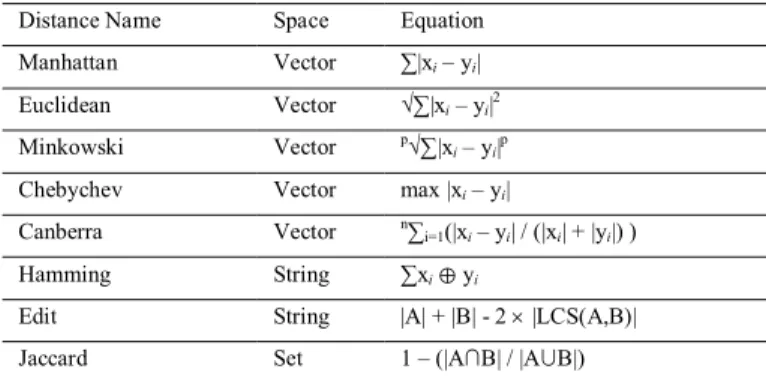
A NNS problem can be defined in two ways, metric and non-metric. The focus of this research paper is on the problems defined on a metric space. The distance formula in non-metric space is converted to a distance in metric space. Different metric distance functions can be defined on the searching space. Table 1 shows a list of formulas along with space that have presented different categorizing and analyzed of NNS.

Table 1. Distance Equations

Distance Name Space Equation Manhattan Vector ∑|xi– yi|

Euclidean Vector √∑|xi– yi|2

Minkowski Vector p_√∑|x

i– yi|p

Chebychev Vector max |xi– yi|

Canberra Vector n_∑

i=1(|xi– yi| / (|xi| + |yi|) )

Hamming String ∑xiΔ yi

Edit String |A| + |B| - 2 u |LCS(A,B)| Jaccard Set 1 – (|A…B| / |A»B|)

2.NNS Data Structures

One of the main parts in NNS is data structure which used in each technique. Now there are different data structures that can use for solving this problem. By paying attention to different applications and data, each of these techniques has to use structure for maintaining, indexing points and searching. Some of these structures are techniques for NNS such as LSH, Ball-Tree, kd-Tree and etc.[2]; and the other are infrastructures in some techniques such as R-tree, R* Tree, B-Tree, X-Tree and etc. A brief overview about some of these data structures is presented as follow.

LSH (Locality Sensitive Hashing) is one of the best algorithms that can be used as a technique. The LSH algorithm is probably the one that has received most attention in practical context. Its main idea is to hash the data points using several hash function so as to ensure that, for each function the probability of collision is much higher for points which are close to each other than for those which are far apart.

In LSH algorithm at first preprocessing should have been done. In preprocessing all data points hash by all functions and determine their buckets. In searching step query point q is hashed and after determining buckets all of its data points retrieve as the answer [2,5].

One of the other structures that use as a technique is kd-Tree that creates for a set with n points in d-dimensional space recursive. kd-Tree and its variance remain probably the most popular data structure used for searching in multidimensional space at least in main memory. In this structure, in each step the existence space is divided by paying attention to points dimensions.

(3)

This division is continued recursively until that in each zone just a point is remained. Finally the data structure that produced is a binary tree with n level and depth. For searching nearest neighbor a circle is drawn with query

point q as center and | p – q | as radius that p is in query point q zone. With assisting of points that are interfered with

the circle, the radius and p are updated. This operation is continued until up to dating is possible and finally NN is reported [6-9].

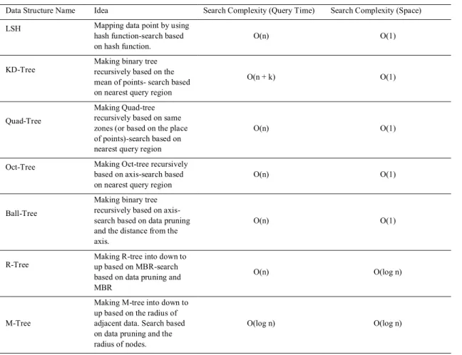
Table 2. Computational Complexity of Data Structures

Data Structure Name Idea Search Complexity (Query Time) Search Complexity (Space) LSH Mapping data point by using

hash function-search based on hash function.

O(n) O(1)

KD-Tree Making binary tree _{recursively based on the} mean of points- search based on nearest query region

O(n + k) O(1)

Quad-Tree

Making Quad-tree recursively based on same zones (or based on the place of points)-search based on nearest query region

O(n) O(1)

Oct-Tree Making Oct-tree recursively based on axis-search based on nearest query region

O(n) O(1)

Ball-Tree

Making binary tree recursively based on axis-search based on data pruning and the distance from the axis.

O(n) O(1)

R-Tree Making R-tree into down to up based on MBR-search based on data pruning and MBR

O(n) O(log n)

M-Tree

Making M-tree into down to up based on the radius of adjacent data. Search based on data pruning and the radius of nodes.

O(log n) O(log n)

Quad-Tree and Oct-Tree act similar to kd-Tree, as Quad–Tree used in two dimensional spaces and for creating

tree in it, each zone in each repetition is divided to four parts. Oct-Tree used in 3D and each zone in each repetition

is divided to eight parts. Searching operation in these two structures are similar to kd-Tree [10 – 14].

Also we can point to Ball-Tree [15, 16]. A Ball-Tree is a binary tree where each node represents a set of points, called Pts(N). Given a data set, the root node of a Ball-Tree represents the full set of points in the data set. A node can be either a leaf node or a non-leaf node. A leaf node explicitly contains a list of the points represented by the node. A non-leaf node has two children nodes: N.child1and N.child2.

Pts(N.child1) … Pts(N.child2) = f

Pts(N.child1) » Pts(N.child2) = Pts(N)

Points are organized spatially. Each node has a distinguished point called a Pivot. Depending on the implementation, the Pivot may be one of the data points, or it may be the centroid of Pts(N). Each node records the maximum distance of the points it owns to its pivot.

For searching in this tree, the algorithms such as KNS1, KNS2, KNS3 and KNSV can be used. As these algorithms have rules for pruning points. One of the other important extant structures is R-Tree that also named

(4)

spatial access method. R-trees are a generalized B-tree. R-trees can handle multidimensional data. R-Trees can be used in Temporal and Spatial Data and also in commercial database management systems such as Oracle, MySQL and Postgre SQL. Furthermore in spaces which points are moveable, R-Tree is one of the most usable structures. This tree one of data structures which operate based on local indexing. This local indexing is defined as rectangular vicinity named MBR (Minimum Bounding Rectangle). MBR is the smallest local rectangle that contains its all points and subset nodes. R-Tree uses three concept distance for searching: MinDist, MaxDist and MinMaxDist. Also this tree is a balance tree and all of its leaves are in the same level. For R-Tree there are two algorithms for searching nearest neighbor to HS and RKV that HS is a breadth search Algorithm and RKV is a branch and bound algorithm that use depth search [17 - 21].

Another structure that can be used for NNS is M-Tree that is inspirited from R-Tree and B-Tree with the difference that pay more attention to memory and I/O.M-Tree is defined by paying attention to different situation and tries to prune more points. Searching in this is similar to R-Tree but with priority queue searching algorithm is optimum. For indexing points in metric space M-Tree is used such as VP-Trees, Cover-Trees, MVP-Trees and BK-Trees [22, 23]. And another structures for NNS that is created by R-Tree idea are R*-Tree, R+-Tree, TPR-Tree, X-Tree, SS-X-Tree, SR-X-Tree, A-Tree and BD-Tree. At the end of this section the complexity of some of the structures are compared in table 2.

3.Nearest Neighbor Search Technique

One of the most important reasons that have made it pervasive is widespread of application and its extent. This wide spreading caused heterogeneous data, conditions and system environment and made the solution hard. So it is necessary to create a technique that has the best result. With this reason for solving NNS problem, different technique with different approach has been created. Each of these techniques can be divided to two parts. The first part consists suitable structure for indexing and maintaining data points that is discussed in the last section. It is necessary to mention that some of these structures itself can be used as a technique for NNS, such as KD-Tree, Ball-Tree and LSH.

The second part consists a suitable algorithm for finding the nearest points to query point q. linear searching and kNN can be mentioned as simple and first techniques [2]. In linear searching for each query point q, its distance from all points in S is calculated and each point that has the lowest distance is chosen as a result. The main problem in this technique is unsalable that in high dimensional or by increasing the points in space, the speed of searching is really decreased.

kNN technique for the first time in T. M. Cover et. al. [24] has been presented for classification and used simple algorithm. A naive solution for the NNS problem is using linear search method that computes distance from the query to every single point in the dataset and returns the k closest points. This approach is guaranteed to find the exact nearest neighbors. However, this solution can be expensive for massive datasets. By paying attention to this

initial algorithm, different techniques have been presented that each of them tries to improve kNN’s performance. In

present study, a new, suitable and comparable categorizing from these techniques is presented. By paying attention to this, these techniques have been categorized to different groups that are discussed as follow.

3.1.Weighted techniques

In such these groups of techniques, by give weight to points the effect of each of them on final result is denoted that one of the main applications of this group is its usage in information classification. Some of these techniques are mentioned as follow: Weighted k-Nearest Neighbor (Weighted-kNN), Modified k-Nearest Neighbor (Modified-kNN) and Pseudo k-Nearest Neighbor (Pseudo-(Modified-kNN).

Surveying the position of each point compare to other points for query point q is one of the most application methods which kNN use it. In this technique if distance is defined as weight, it names distance Weighted-kNN. Usually each of the points has different distance from query point q, so nearer points have more effects. In this technique calculating weight based on distance of points S. A. Dudani et. al [25, 26].

(5)

If space has imbalance data, it is better to use Neighbor Weighted-kNN instance of Weighted-kNN. If in a set of data same of the classes have many members in compare to others, its score very high and so more query belong to this class. For solving this problem it is necessary that the classes with more members gain low weight and the classes with less members gain high weight. The weight for each class calculated in S. Tan et. al [27, 28].

For example in point classification for presenting better answer instead of distance, product of distance and weight must be used. Here by paying attention to space weight is calculated by one of these techniques. In more problems choosing neighbors based on distance have some problems such as low Accuracy and incorrect answers. Modified-kNN method which use for classification, tries to solve these problems. At first a preprocessing is done on all of the points and gives a validity value to each point. This value defines based on each point H nearest neighbor. 3.2.Reductional techniques

One of the necessary needs in data processing is extra data and its suitable summarize. This is introduced in spaces which has massive data or data that need high memory. These techniques caused improving performance of systems by decreasing data. Condensed k-Nearest Neighbor (Condensed-kNN), Reduced k-Nearest Neighbor (Reduced-kNN), Model Based k-Nearest Neighbor (ModelBased-kNN) and Clustered k-Nearest Neighbor

(Clustered-kNN) are discussed in this section [29 – 35].

Data that are considered as unnecessary information, identical with other data, are deleted in Condensed-kNN. There are two approaches, A) It is assumed that the data are labeled. Then instead of saving the data along with their classes, sample data is saved so that there will be no duplicate data in the dataset. B) Data might be without label; thus the desired cluster can be found by clustering and sample data is obtained from the center of the cluster. kNN

operation then, is carried out on the remainder of the data [29 – 31].

Another approach, which uses the nearest neighbor to reduce information volume, is Reduced-kNN (a developed version of condensed-kNN). In addition to removing identical data, null data is also deleted. This even shrinks more the data volume and facilitates the system response to queries. Moreover, smaller memory space is required for processing. One of the drawbacks is increase in complexity of computations and costs of execution of the algorithm consequently. In general, these two approaches are time consuming [29, 32].

The next technique to reduce information volume is ModelBased-kNN. As the technique dictates, a data model is first extracted from the information and replaces the data. This removes a great portion of the information volume. It is noticeable, however, that the data model needs to resemble well the whole data. In place of the whole data, for instance, one may use the data that show the points (usually the central point), number of the member, distance of

the farthest data from the resemblance and the class label in some cases. Modelbased-kNN employs “largest local

neighborhood” and “largest global neighborhood” to create a simpler structure and definition of the model so that the data are modeled step by step [33, 34].

3.3.Additive Techniques

In this group of techniques it is tried to increase system operation accuracy by increasing data volume. Another aim of these techniques is paying attention to all of points together that can affect each other. Nearest Feature Line (NFL), Local Nearest Neighbor (Local-kNN), Center Based Nearest Neighbor (CenterBased-kNN) and Tunable

Nearest Neighbor (Tunable-kNN) are discussed in this section [36 – 41].

When the number of points for classification is not enough, accuracy of the final result is unacceptable. It is necessary to have another technique for increasing data volume and the accuracy consequently. One answer, Euclidean and 2D spaces, is NFL technique. By converting each two points in a class (future points) into a line, not only NFL increases the data volume but it adds to effect of the points in each class. Future points (FP) symbolize features of a class and there are two FPs at least in each class. The lines drawn between the two FPs are called future lines (FL). Instead of calculating distance between q and other data points, perpendicular distance between q and each FL is measured (Figure 1a).

With high efficiency of the technique in small dataset, by increasing size of dataset the computation complexities is increased. There is a risk of wrong determination of nearest FL in NFL for distant q and FPs (Figure 1b). Figure

(6)

Fig. 1. (a) Mapping Query Point on Future Line [36], (b) Nearest Future Line Drawback in Classification [38]

To deal with the drawback, Local-kNN was introduced, so that FPs are chosen among k nearest neighbors of q in each class. This ensures accurate determination of nearest FL, though great deal of computation is required. For classification, first kNN for each class is computed.

If k=2, distance between q and the FL is created from 2NN of each class and if k = 3, distance between q to future plane created from 3NN of each class are obtained. Finally, the class with shortest distance to q is taken as the result 3.4.Reverse Techniques

Reverse techniques are the most important and most application techniques in NNS. This group is variety that in present paper some of them are discussed. In this group of techniques the approach of problem is changed and data points are taken more attention than query points. Reverse Nearest Neighbor (Reverse-kNN) and Mutual Nearest

Neighbor (Mutual-kNN) are described in this section [42 – 48].

The straightest way to find reserve-kNN of query point q is to calculated the nearest point in the dataset based on the distance equation of each p; this creates regions centered by p with radius of . Then, when point q is located in one of the regions, the point p in the regions is the answer. Noticeably, the for L2-norm and LĞ-norm are circle and rectangular respectively. In spite of kNN, Reserve-kNN technique may have empty set as answer and given the distance function and dimension of the data, number of points in the set is limited. If L2-norm is the case, for instance, we have 6 and 12 points at most under 3D and 2D spaces respectively. For LĞ-norm there are equal points. A comparison between kNN and Reserve-kNN is carried out in follow [42-47].

(7)

3.5.Continuous Techniques

Techniques that are presented in this section are suitable for points that are introduced in continuous space instead of discrete space. In this section continuous Nearest Neighbor (Continuous -kNN) and Range Nearest Neighbor (Range-kNN) are evaluated [49, 50].

3.6.Principal Axis Techniques

In this group of techniques data environment is divided in several subset. Each these sets have an Axis which data are mapped on them. In this section Principal Axis Nearest Neighbor (Principal Axis-kNN) and Orthogonal Nearest Neighbor (Orthogonal-kNN) are introduced [51-54].

Fig 3(a). Partition of a 2D Data Set using a Principal Axis Tree[51], (b)Pruning Data Set using a Principal Axis Tree [51]

One of the techniques to find kNN is Principal Axis-kNN. As the method implies, the dataset is divided into several subsets. The dividing is continued until every subset is smaller than a specific threshold (e.g. 'nc'). Along

with dividing, a principle axis tree (PAT) is developed so that the leaf’s nodes have 'nc' data points at most (Figure 3a). Each node in PAT has a principle axis which is used for mapping data and calculating distance as well as pruning. For search operation, first the node where the q is located is searched through a binary query. Then, the node and/or sibling nodes are searched to find kNN of query point q (Figure 3b). To have faster process, some regions are pruned using the principle axis [51, 52].

4.Assessment and Comparison of Techniques

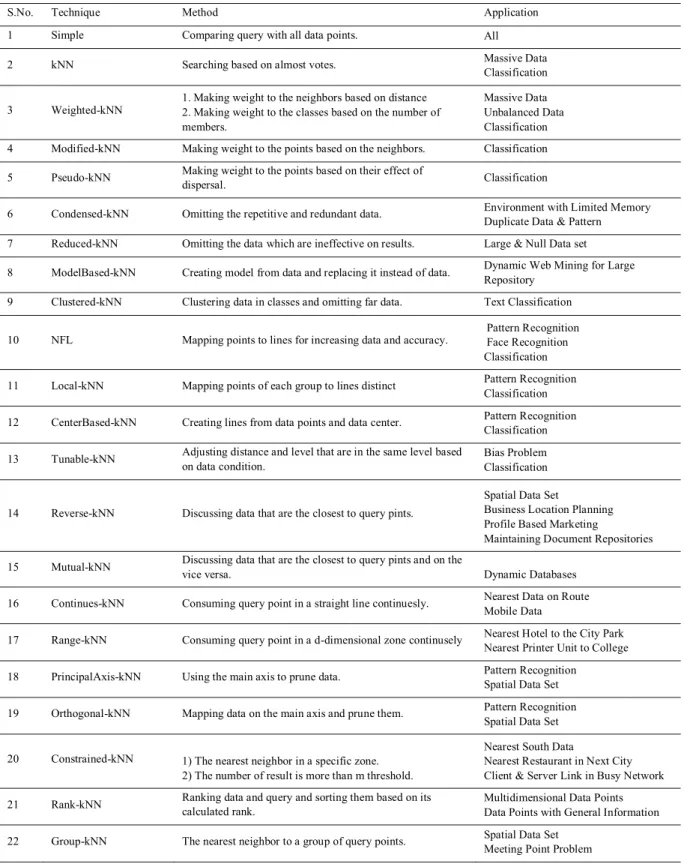
Each of the presented techniques in this paper is suitable for using in spaces with special data but it can't be used generally. So in this section, these techniques are compared and evaluated. These comparison and evaluation are presented. In table 3 presented each technique's idea and applications.

(8)

Table 3. Nearest Neighbor Techniques

S.No. Technique Method Application

1 Simple Comparing query with all data points. All

2 kNN Searching based on almost votes. Massive Data Classification

3 Weighted-kNN 1. Making weight to the neighbors based on distance _{2. Making weight to the classes based on the number of} members.

Massive Data Unbalanced Data Classification 4 Modified-kNN Making weight to the points based on the neighbors. Classification

5 Pseudo-kNN Making weight to the points based on their effect of _dispersal. Classification

6 Condensed-kNN Omitting the repetitive and redundant data. Environment with Limited Memory Duplicate Data & Pattern 7 Reduced-kNN Omitting the data which are ineffective on results. Large & Null Data set

8 ModelBased-kNN Creating model from data and replacing it instead of data. Dynamic Web Mining for Large _Repository

9 Clustered-kNN Clustering data in classes and omitting far data. Text Classification

10 NFL Mapping points to lines for increasing data and accuracy. Pattern Recognition Face Recognition Classification

11 Local-kNN Mapping points of each group to lines distinct Pattern Recognition Classification

12 CenterBased-kNN Creating lines from data points and data center. Pattern Recognition _{Classification}

13 Tunable-kNN Adjusting distance and level that are in the same level based on data condition.

Bias Problem Classification

14 Reverse-kNN Discussing data that are the closest to query pints.

Spatial Data Set

Business Location Planning Profile Based Marketing

Maintaining Document Repositories

15 Mutual-kNN Discussing data that are the closest to query pints and on the

vice versa. Dynamic Databases

16 Continues-kNN Consuming query point in a straight line continuesly. Nearest Data on Route _{Mobile Data}

17 Range-kNN Consuming query point in a d-dimensional zone continusely Nearest Hotel to the City Park Nearest Printer Unit to College

18 PrincipalAxis-kNN Using the main axis to prune data. Pattern Recognition Spatial Data Set

19 Orthogonal-kNN Mapping data on the main axis and prune them. Pattern Recognition Spatial Data Set

20 Constrained-kNN 1) The nearest neighbor in a specific zone. 2) The number of result is more than m threshold.

Nearest South Data

Nearest Restaurant in Next City Client & Server Link in Busy Network

21 Rank-kNN Ranking data and query and sorting them based on its _{calculated rank.} Multidimensional Data Points Data Points with General Information

(9)

5.Conclusion

In this paper, the metric and non-metric spaces are defined. The first one is used in NNS problem. Diverse distance formulas which are used in this problem to find the nearest data point are described and then different structures are introduced. These structures are used for indexing points and making the searching operation faster. Some of these structures such as: Ball-Tree, LSH and KD-Tree are considered as technique for NNS problem. Finally, a new categorization based on the functionality of different techniques for NNS problem is introduced. Techniques with similar functionality are grouped together in this categorization. This categorization consists of six groups; Weighted, Reductional, Additive, Reverse, Continuous, Principal Axis techniques. In each group, the main features of the group are described and each technique is introduced briefly. Finally, a complete comparison of these techniques is done.

References

1. Andoni, Nearest Neighbor Search - the Old, the New, and the Impossible, Ph.D. dissertation, Electrical Engineering and Computer Science, Massachusetts Institute of Technology, 2009.

2. G. Shakhnarovich, T. Darrell, and P. Indyk, Nearest Neighbor Methods in Learning and Vision : Theory and Practice, March 2006. 3. N. Bhatia and V. Ashev, Survey of Nearest Neighbor Techniques, International Journal of Computer Science and Information Security,

8(2), 2010, pp. 1-4.

4. S. Dhanabal and S. Chandramathi, A Review of various k-Nearest Neighbor Query Processing Techniques, Computer Applications. 31(7), 2011, pp. 14-22.

5. A. Rajaraman and J. D. Ullman. Mining of Massive Datasets, December 2011.

6. R. F. Sproull, Refinements to Nearest-Neighbor Searching in k Dimensional Trees, Algorithmica. 6(4), 1991, pp. 579-589.

7. J. L. Bentley, Multidimensional binary search trees Used for Associative Searching, Communications of the ACM. 18(9), 1975, pp. 509-517.

8. R. Panigrahy, An Improved Algorithm Finding Nearest Neighbor Using Kd-Trees, in 8th Latin American conference on Theoretical informatics, Bzios, Brazil, 2008, pp. 387-398.

9. A. Nuchter, K. Lingemann, and J. Hertzberg, Cached KD Tree Search for ICP Algorithms, in 6th International Conference on 3 -D Digital Imaging and Modeling, Montreal, Quebec, Canada, 2007, pp. 419-426.

10. V. Gaede and O. Gunther, Multidimensional access methods, ACM Computing Surveys. 30(2), 1998, pp. 170-231. 11. H. Samet, The Quadtree and Related Hierarchical Data Structures, ACM Computing Surveys. 16(2), 1984, pp. 187-260.

12. J. Tayeb, O. Ulusoy, and O. Wolfson, A Quadtree Based Dynamic Attribute Indexing Method, The Computer Journal. 41(3), 1998,pp. 185-200.

13. C. A. Shaffer and H. Samet, Optimal Quadtree Construction Algorithms, Computer Vision, Graphics, and Image Processing. 37(3), 1987, pp. 402-419.

14. D. Meagher, Geometric Modeling Using Octree Encoding, Computer Graphics and Image Processing. 19(2), 1982, pp. 129-147.

15. T. Liu, A. W. Moore, and A. Gray, New Algorithms for Efficient High Dimensional Nonparametric Classification, The Journal of Machine Learning Research. 7(1), 2006, pp. 1135–1158.

16. S. M. Omohundro, Five Balltree Construction Algorithms, International Computer Science Institute, Berkeley, California, USA, Tech, 1989.

17. Y. Manolopoulos, A. Nanopoulos, A. N. Papadopoulos, and Y. Theodoridis, R-Trees: Theory and Applications, November 2005. 18. A. Guttman, R-Trees: A dynamic index structure for spatial searching, ACM SIGMOD Record. 14(2), 1984, pp. 47-57. 19. M. K. Wu, Evaluation of R-trees for Nearest Neighbor Search, M.Sc. thesis, Computer Science, University of Houston, 2006. 20. N. Roussopoulos, S. Kelley, and F. Vincent, Nearest Neighbor Queries, ACM SIGMOD Record. 24(2), 1995, pp.71-79.

21. M. Adler and B. Heeringa, Search Space Reductions for Nearest Neighbor Queries, in 5th international conference on Theory and applications of models of computation, Xian, China, 2008, pp. 554-568.

22. P. Ciaccia, M. Patella, and P. Zezula, M-tree: An Efficient Access Method for Similarity Search in Metric Spaces, in 23rd Very Large Data Bases Conference, Athens, Greece, 1997.

23. T. Skopal, Pivoting M-tree: A Metric Access Method for Efficient Similarity Search, in Dateso 2004 Annual International Workshop on Databases, Texts, Specifications and Objects, Desna, Czech Republic, 2004, pp. 27-37.

24. T. M. Cover and P. E. Hart, Nearest Neighbor Pattern Classification, IEEE Transactions on Information Theory. 13(1), 1967, pp. 21-27. 25. S. A. Dudani, The Distance-Weighted k-Nearest-Neighbor Rule, IEEE Transactions on Systems, Man and Cybernetics. 6(4), 1976, pp.

325-327.

26. T. Bailey and A. K. Jain, A Note on Distance-Weighted k-Nearest Neighbor Rules, IEEE Transactions on Systems, Man and Cybernetics. 8(4), 1978, pp. 311-313.

(10)

28. K. Hechenbichler and K. Schliep, Weighted k-Nearest-Neighbor Techniques and Ordinal Classification, Collaborative Research Center, LMU University, Munich, Germany, Tech, 2006.

29. V. Lobo, Ship Noise Classification: A Contribution to Prototype Based Classifier Design, Ph.D. dissertation, College of Science and Technology, New University of Lisbon, 2002.

30. P. E. Hart, The Condensed Nearest Neighbor Rule, IEEE Transactions on Information Theory. 14(3), 1968, pp. 515-516.

31. F. Angiulli, Fast Condensed Nearest Neighbor Rule, in 22nd International Conference on Machine Learning, Bonn, Germany, 2005, pp. 25-32.

32. G. W. Gates, The Reduced Nearest Neighbor Rule, IEEE Transactions on Information Theory. 18(3), 1972, pp. 431-433.

33. G. Guo, H. Wang, D. Bell, Y. Bi, and K. Greer, KNN Model-Based Approach in Classification, in OTM Confederated International Conferences on the Move to Meaningful Internet Systems, Catania, Sicily, Italy, 2003, pp. 986-996.

34. G. Guo, H. Wang, D. Bell, Y. Bi, and K. Greer, An KNN Model-Based Approach and its Application in Classification in Text Categorization, in 5th International Conference on Computational Linguistics and Intelligent Text Processing, Seoul, Korea, 2004, pp. 559-570.

35. Z. Yong, L. Youwen, and X. Shixiong, An Improved KNN Text Classification Algorithm Based on Clustering, Journal of Computers. 4(3), 2009, pp. 230-237.

36. S. Z. Li and J. Lu, Face Recognition Using the Nearest Feature Line Method, IEEE Transactions on Neural Networks. 10(2), 1999, pp. 439-443.

37. S. Z. Li, K. L. Chan, and C. Wang, Performance Evaluation of the Nearest Feature Line Method in Image Classification and Retr ieval, IEEE Transactions on Pattern Analysis and Machine Intelligence. 22(11), 2000, pp. 1335-1339.

38. W. Zheng, L. Zhao, and C. Zou, Locally nearest neighbor classifiers for pattern classification, Pattern Recognition. 37(6), 2004, pp. 1307-1309.

39. Q. B. Gao and Z. Z. Wang, Center Based Nearest Neighbor Classifier, Pattern Recognition. 40(1), 2007, pp. 346-349.

40. Y. Zhou, C. Zhang, and J. Wang, Tunable Nearest Neighbor Classifier, in 26th DAGM Symposium on Artificial Intelligence, Tubing en, Germany, 2004, pp. 204-211.

41. Y. Zhou, C. Zhang, and J. Wang, Extended Nearest Feature Line Classifier, in 8th Pacific Rim International Conference on Artificial Intelligence, Auckland, New Zealand, 2004, pp. 183-190.

42. F. Korn and S. M. ukrishnan, Influence Sets Based on Reverse Nearest Neighbor Queries, ACM SIGMOD Record. 29(2), 2000, pp. 20 1-212.

43. C. Yang and K. I. Lin, An Index Structure for Efficient Reverse Nearest Neighbor Queries, in 17th International Conference on Data Engineering, Heidelberg, Germany, 2001, pp. 485-492.

44. R. Benetis, C. S. Jensen, G. Karciauskas, and S. Saltenis, Nearest Neighbor and Reverse Nearest Neighbor Queries for Moving Objects, The VLDB Journal. 15(3), 2006, pp. 229-249.

45. Y. Tao, M. L. Yiu, and N. Mamoulis, Reverse Nearest Neighbor Search in Metric Spaces, IEEE Transactions on Knowledge and Data Engineering. 18(9), 2006, pp. 1239-1252.

46. I. Stanoi, D. Agrawal, and A. E. Abbadi, Reverse Nearest Neighbor Queries for Dynamic Databases, in ACM SIGMOD Workshop on Research Issues in Data Mining and Knowledge Discovery, Dallas, Texas, USA, 2000, pp.44-53.

47. E. Achtert, C. Bohm, P. Kroger, P. Kunath, M. Renz, and A. Pryakhin, Efficient Reverse k-Nearest Neighbor Search in Arbitrary Metric Spaces, in ACM SIGMOD International Conference on Management of Data, Chicago, Illinois, USA, 2006, pp. 515-526.

48. Y. Gao, B. Zheng, G. Chen, and Q. Li, On Efficient Mutual Nearest Neighbor Query Processing in Spatial Databases, Data & Knowledge Engineering. 68(8), 2009, pp. 705-727.

49. Y. Tao, D. Papadias, and Q. Shen, Continuous Nearest Neighbor Search, in 28th international conference on Very Large Data Bases, Hong Kong, China, 2002, pp. 287-298.

50. H. Hu and D. L. Lee, Range Nearest-Neighbor Query, IEEE Transactions on Knowledge and Data Engineering. 18(1), 2006, pp. 78-91. 51. J. McNames, A Fast Nearest-Neighbor Algorithm Based on a Principal Axis Search Tree, IEEE Transactions on Pattern Analysis and

Machine Intelligence. 23(9), 2001, pp. 964-976.

52. B. Wang and J. Q. Gan, Integration of Projected Clusters and Principal Axis Trees for High-Dimensional Data Indexing and Query, in 5th International Conference on Intelligent Data Engineering and Automated Learning, Exeter, UK, 2004, 2001, pp. 191–196.

53. Y. C. Liaw, M. L. Leou, and C. M. Wu, Fast Exact k Nearest Neighbors Search Using an Orthogonal Search Tree, Pattern Recognition. 43(6), 2010, pp. 2351-2358.

54. Y. C. Liaw, C. M. Wu, and M. L. Leou, Fast k Nearest Neighbors Search Using Modified Principal Axis Search Tree, Digital Signal Processing. 20(5), 2010 pp. 1494-1501.