Second-Order Stochastic Optimization for Machine Learning
in Linear Time
Naman Agarwal [email protected]
Computer Science Department Princeton University
Princeton, NJ 08540, USA
Brian Bullins [email protected]
Computer Science Department Princeton University
Princeton, NJ 08540, USA
Elad Hazan [email protected]
Computer Science Department Princeton University
Princeton, NJ 08540, USA
Editor:Tong Zhang
Abstract
First-order stochastic methods are the state-of-the-art in large-scale machine learning op-timization owing to efficient per-iteration complexity. Second-order methods, while able to provide faster convergence, have been much less explored due to the high cost of computing the second-order information. In this paper we develop second-order stochastic methods for optimization problems in machine learning that match the per-iteration cost of gradient based methods, and in certain settings improve upon the overall running time over pop-ular first-order methods. Furthermore, our algorithm has the desirable property of being implementable in time linear in the sparsity of the input data.
Keywords: second-order optimization, convex optimization, regression
1. Introduction
In recent literature stochastic first-order optimization has taken the stage as the primary workhorse for training learning models, due in large part to its affordable computational costs which are linear (in the data representation) per iteration. The main research effort devoted to improving the convergence rates of first-order methods have introduced elegant ideas and algorithms in recent years, including adaptive regularization (Duchi et al., 2011), variance reduction (Johnson and Zhang, 2013; Defazio et al., 2014), dual coordinate ascent (Shalev-Shwartz and Zhang, 2013), and many more.
In contrast, second-order methods have typically been much less explored in large scale machine learning (ML) applications due to their prohibitive computational cost per itera-tion which requires computaitera-tion of the Hessian in addiitera-tion to a matrix inversion. These operations are infeasible for large scale problems in high dimensions.
c
In this paper we propose a family of novel second-order algorithms, LiSSA (Linear time Stochastic Second-Order Algorithm) for convex optimization that attain fast convergence rates while also allowing for an implementation with linear time per-iteration cost, matching the running time of the best known gradient-based methods. Moreover, in the setting where the number of training examplesmis much larger than the underlying dimensiond, we show that our algorithm has provably faster running time than the best known gradient-based methods.
Formally, the main optimization problem we are concerned with is the empirical risk minimization (ERM) problem:
min
x∈Rdf(x) = minx∈ Rd
(
1 m
m
X
k=1
fk(x) +R(x)
)
where each fk(x) is a convex function and R(x) is a convex regularizer. The above
opti-mization problem is the standard objective minimized in most supervised learning settings. Examples include logistic regression, SVMs, etc. A common aspect of many applications of ERM in machine learning is that the loss function fi(x) is of the form l(x>vi, yi) where
(vi, yi) is theithtraining example-label pair. We call such functions generalized linear
mod-els (GLM) and will restrict our attention to this case. We will assume that the regularizer is an`2 regularizer,1 typically kxk2.
Our focus is second-order optimization methods (Newton’s method), where in each iteration, the underlying principle is to move to the minimizer of the second-order Taylor approximation at any point. Throughout the paper, we will let ∇−2f(x) ,
∇2f(x)−1
. The update of Newton’s method at a point xtis then given by
xt+1 =xt− ∇−2f(xt)∇f(xt). (1)
Certain desirable properties of Newton’s method include the fact that its updates are in-dependent of the choice of coordinate system and that the Hessian provides the necessary regularization based on the curvature at the present point. Indeed, Newton’s method can be shown to eventually achieve quadratic convergence (Nesterov, 2013). Although Newton’s method comes with good theoretical guarantees, the complexity per step grows roughly as Ω(md2+dω) (the former term for computing the Hessian and the latter for inversion, where ω≈2.37 is the matrix multiplication constant), making it prohibitive in practice. Our main contribution is a suite of algorithms, each of which performs an approximate Newton update based on stochastic Hessian information and is implementable in linear O(d) time. These algorithms match and improve over the performance of first-order methods in theory and give promising results as an optimization method on real world data sets. In the following we give a summary of our results. We propose two algorithms, LiSSA and LiSSA-Sample.
LiSSA: Algorithm 1 is a practical stochastic second-order algorithm based on a novel estimator of the Hessian inverse, leading to an efficient approximate Newton step (Equation 1). The estimator is based on the well known Taylor approximation of the inverse (Fact 2) and is described formally in Section 3.1. We prove the following informal theorem about LiSSA.
Theorem 1 (Informal) LiSSA returns a point xt such that f(xt) ≤ minx∗f(x∗) +ε in total time
˜ O
(m+S1κ)dlog
1 ε
whereκis the underlying condition number of the problem andS1 is a bound on the variance
of the estimator.
The precise version of the above theorem appears as Theorem 7. In theory, the best bound we can show for S1 is O(κ2); however, in our experiments we observe that setting S1 to be a small constant (often 1) is sufficient. We conjecture that S1 can be improved to O(1) and leave this for future work. If indeedS1 can be improved toO(1) (as is indicated by our experiments), LiSSA enjoys a convergence rate comparable to first-order methods. We provide a detailed comparison of our results with existing first-order and second-order methods in Section 1.2. Moreover, in Section 7 we present experiments on real world data sets that demonstrate that LiSSA as an optimization method performs well as compared to popular first-order methods. We also show that LiSSA runs in time proportional to input sparsity, making it an attractive method for high-dimensional sparse data.
LiSSA-Sample: This variant brings together efficient first-order algorithms with matrix sampling techniques (Li et al., 2013; Cohen et al., 2015) to achieve better runtime guarantees than the state-of-the-art in convex optimization for machine learning in the regime when m > d. Specifically, we prove the following theorem:
Theorem 2 (Informal) LiSSA-Sample returns a pointxtsuch thatf(xt)≤minx∗f(x∗)+
εin total time
˜
Om+√κddlog2
1 ε
log log
1 ε
.
The above result improves upon the best known running time for first-order methods achieved by acceleration when we are in the setting where κ > m >> d. We discuss the implication of our bounds and further work in Section 1.3.
In all of our results stated aboveκcorresponds to the condition number of the underlying problem. In particular we assume some strong convexity for the underlying problem. This is a standard assumption which is usually enforced by the addition of the `2 regularizer. In stating our results formally we stress on the nuances between different notions of the condition number (ref. Section 2.1), and we state our results precisely with respect to these notions. In general, all of our generalization/relaxations of the condition number are smaller than 1λ whereλis the regularization parameter, and this is usually taken to be the condition number of the problem. The condition of strong convexity has been relaxed in literature by introducing proximal methods. It is an interesting direction to adapt our results in those setting which we leave for future work.
While it is possible that this regime is less interesting for generalization, in this paper we focus on the optimization problem itself.
We further consider the special case when the function f is self-concordant. Self-concordant functions are a sub-class of convex functions which have been extensively stud-ied in convex optimization literature in the context of interior point methods (Nemirovski, 2004). For self-concordant functions we propose an algorithm (Algorithm 5) which achieves linear convergence with running time guarantees independent of the condition number. We prove the formal running time guarantee as Theorem 25.
We believe our main contribution to be a demonstration of the fact that second-order methods are comparable to, or even better than, first-order methods in the large data regime, in both theory and practice.
1.1 Overview of Techniques
LiSSA: The key idea underlying LiSSA is the use of the Taylor expansion to construct a natural estimator of the Hessian inverse. Indeed, as can be seen from the description of the estimator in Section 3.1, the estimator we construct becomes unbiased in the limit as we include additional terms in the series. We note that this is not the case with estimators that were considered in previous works such as that of Erdogdu and Montanari (2015), and so we therefore consider our estimator to be more natural. In the implementation of the algorithm we achieve the optimal bias/variance trade-off by truncating the series appropriately.
An important observation underlying our linear time O(d) step is that for GLM func-tions, ∇2f
i(x) has the form αviv>i where α is a scalar dependent on vi>x. A single step
of LiSSA requires us to efficiently compute ∇2f
i(x)b for a given vector b. In this case it
can be seen that the matrix-vector product reduces to a vector-vector product, giving us an O(d) time update.
LiSSA-Sample: LiSSA-Sample is based on Algorithm 2, which represents a general family of algorithms that couples the quadratic minimization view of Newton’s method with any efficient first-order method. In essence, Newton’s method allows us to reduce (up to log log factors) the optimization of a general convex function to solving intermediate quadratic or ridge regression problems. Such a reduction is useful in two ways.
First, as we demonstrate through our algorithm LiSSA-Sample, the quadratic nature of ridge regression problems allows us to leverage powerful sampling techniques, leading to an improvement over the running time of the best known accelerated first-order method. On a high level this improvement comes from the fact that when solving a system of m linear equations in ddimensions, a constant number of passes through the data is enough to reduce the system to O(dlog(d)) equations. We carefully couple this principle and the computation required with accelerated first-order methods to achieve the running times for LiSSA-Sample. The result for the quadratic sub-problem (ridge regression) is stated in Theorem 15, and the result for convex optimization is stated in Theorem 16.
improve-ment; however, in practice we believe that this could be significant and lead to runtime improvements.2
To achieve the bound for LiSSA-Sample we extend the definition and procedure for sampling via leverage scores described by Cohen et al. (2015) to the case when the matrix is given as a sum of PSD matrices and not just rank one matrices. We reformulate and reprove the theorems proved by Cohen et al. (2015) in this context, which may be of independent interest.
1.2 Comparison with Related Work
In this section we aim to provide a short summary of the key ideas and results underlying op-timization methods for large scale machine learning. We divide the summary into three high level principles: first-order gradient-based methods, second-order Hessian-based methods, and quasi-Newton methods. For the sake of brevity we will restrict our summary to results in the case when the objective is strongly convex, which as justified above is usually ensured by the addition of an appropriate regularizer. In such settings the main focus is often to obtain algorithms which have provably linear convergence and fast implementations.
First-Order Methods: First-order methods have dominated the space of optimization algorithms for machine learning owing largely to the fact that they can be implemented in time proportional to the underlying dimension (or sparsity). Gradient descent is known to converge linearly to the optimum with a rate of convergence that is dependent upon the condition number of the objective. In the large data regime, stochastic first-order meth-ods, introduced and analyzed first by Robbins and Monro (1951), have proven especially successful. Stochastic gradient descent (SGD), however, converges sub-linearly even in the strongly convex setting. A significant advancement in terms of the running time of first-order methods was achieved recently by a clever merging of stochastic gradient descent with its full version to provide variance reduction. The representative algorithms in this space are SAGA (Roux et al., 2012; Defazio et al., 2014) and SVRG (Johnson and Zhang, 2013; Zhang et al., 2013). The key technical achievement of the above algorithms is to relax the running time dependence on m (the number of training examples) and κ (the condition number) from a product to a sum. Another algorithm which achieves similar running time guarantees is based on dual coordinate ascent, known as SDCA (Shalev-Shwartz and Zhang, 2013).
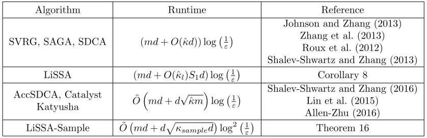
Further improvements over SAGA, SVRG and SDCA have been obtained by applying the classical idea of acceleration emerging from the seminal work of Nesterov (1983). The progression of work here includes an accelerated version of SDCA (Shalev-Shwartz and Zhang, 2016); APCG (Lin et al., 2014); Catalyst (Lin et al., 2015), which provides a generic framework to accelerate first order algorithms; and Katyusha (Allen-Zhu, 2016), which introduces the concept of negative momentum to extend acceleration for variance reduced algorithms beyond the strongly convex setting. The key technical achievement of accelerated methods in general is to reduce the dependence on condition number from linear to a square root. We summarize these results in Table 1.
LiSSA places itself naturally into the space of fast first-order methods by having a running time dependence that is comparable to SAGA/SVRG (ref. Table 1). In LiSSA-Sample we leverage the quadratic structure of the sub-problem for which efficient sampling techniques have been developed in the literature and use accelerated first-order methods to improve the running time in the case when the underlying dimension is much smaller than the number of training examples. Indeed, to the best of our knowledge LiSSA-Sample is the theoretically fastest known algorithm under the condition m >> d. Such an improvement seems out of hand for the present first-order methods as it seems to strongly leverage the quadratic nature of the sub-problem to reduce its size. We summarize these results in Table 1.
Algorithm Runtime Reference
SVRG, SAGA, SDCA (md+O(ˆκd)) log 1ε
Johnson and Zhang (2013) Zhang et al. (2013)
Roux et al. (2012)
Shalev-Shwartz and Zhang (2013)
LiSSA (md+O(ˆκl)S1d) log 1ε
Corollary 8
AccSDCA, Catalyst
Katyusha O˜
md+d√κmˆ log 1ε
Shalev-Shwartz and Zhang (2016) Lin et al. (2015)
Allen-Zhu (2016)
LiSSA-Sample O md˜ +dp
κsampledlog2 1ε Theorem 16
Table 1: Run time comparisons. Refer to Section 2.1 for definitions of the various notions of condition number.
Second-Order Methods: Second-order methods such as Newton’s method have classi-cally been used in optimization in many different settings including development of interior point methods (Nemirovski, 2004) for general convex programming. The key advantage of Newton’s method is that it achieves a linear-quadratic convergence rate. However, naive implementations of Newton’s method have two significant issues, namely that the standard analysis requires the full Hessian calculation which costsO(md2), an expense not suitable for machine learning applications, and the matrix inversion typically requires O(d3) time. These issues were addressed recently by the algorithm NewSamp (Erdogdu and Montanari, 2015) which tackles the first issue by subsampling and the second issue by low-rank pro-jections. We improve upon the work of Erdogdu and Montanari (2015) by defining a more
natural estimator for the Hessian inverse and by demonstrating that the estimator can be computed in time proportional to O(d). We also point the reader to the works of Martens (2010); Byrd et al. (2011) which incorporate the idea of taking samples of the Hessian; however, these works do not provide precise running time guarantees on their proposed algorithm based on problem specific parameters. Second-order methods have also enjoyed success in the distributed setting (Shamir et al., 2014).
algo-rithm (Broyden, 1970; Fletcher, 1970; Goldfarb, 1970; Shanno, 1970). The book of Nocedal and Wright (2006) is an excellent reference for the algorithm and its limited memory vari-ant (L-BFGS). The more recent work in this area has focused on stochastic quasi-Newton methods which were proposed and analyzed in various settings by Schraudolph et al. (2007); Mokhtari and Ribeiro (2014); Byrd et al. (2016). These works typically achieve sub-linear convergence to the optimum. A significant advancement in this line of work was provided by Moritz et al. (2016) who propose an algorithm based on L-BFGS by incorporating ideas from variance reduction to achieve linear convergence to the optimum in the strongly convex setting. Although the algorithm achieves linear convergence, the running time of the algo-rithm depends poorly on the condition number (as acknowledged by the authors). Indeed, in applications that interest us, the condition number is not necessarily a constant as is typically assumed to be the case for the theoretical results in Moritz et al. (2016).
Our key observation of linear time Hessian-vector product computations for machine learning applications provides evidence that in such instances, obtaining true Hessian infor-mation is efficient enough to alleviate the need for quasi-Newton inforinfor-mation via gradients.
1.3 Discussion and Subsequent Work
In this section we provide a brief survey of certain technical aspects of our bounds which have since been improved by subsequent work.
An immediate improvement in terms of S2 ∼ κ (in fact suggested in the original manuscript) was achieved by Bollapragada et al. (2016) via conjugate gradient on a sub-sampled Hessian which reduces this to √κ. A similar improvement can also be achieved in theory through the extensions of LiSSA proposed in the paper. As we show in Section 7, the worse dependence on condition number has an effect on the running time when κ is quite large.3 Accelerated first-order methods, such as APCG (Lin et al., 2014), outperform LiSSA in this regime. To the best of our knowledge second-order stochastic methods have so far not exhibited an improvement in that regime experimentally. We believe a more practical version of LiSSA-Sample could lead to improvements in this regime, leaving this as future work.
To the best of our knowledge the factor of S1=κ2 that appears to reduce the variance of our estimator has yet not been improved despite it beingO(1) in our experiments. This is an interesting question to which partial answers have been provided in the analysis of Ye et al. (2017).
Significant progress has been made in the space of inexact Newton methods based on matrix sketching techniques. We refer the reader to the works of Pilanci and Wainwright (2015); Xu et al. (2016); Cohen (2016); Luo et al. (2016); Ye et al. (2017) and the references therein.
We would also like to comment on the presence of a warm start parameter κM1 in our proofs of Theorems 7 and 15. In our experiments the warm start we required would be quite small (often a few steps of gradient descent would be sufficient) to make LiSSA converge. The warm start does not affect the asymptotic results proven in Theorems 7 and 15 because getting to such a warm start is independent ofε. However, improving this warm start, especially in the context of Theorem 15, is left as interesting future work.
On the complexity side, Arjevani and Shamir (2016) proved lower bounds on the best running times achievable by second-order methods. In particular, they show that to get the faster rates achieved by LiSSA-Sample, it is necessary to use a non-uniform sampling based method as employed by LiSSA-Sample. We would like to remark that in theory, up to logarithmic factors, the running time of LiSSA-Sample is still the best achieved so far in the setting m >> d. Some of the techniques and motivations from this work were also generalized by the authors to provide faster rates for a large family of non-convex optimization problems (Agarwal et al., 2017).
1.4 Organization of the Paper
The paper is organized as follows: we first present the necessary definitions, notations and conventions adopted throughout the paper in Section 2. We then describe our estimator for LiSSA, as well as state and prove the convergence guarantee for LiSSA in Section 3. After presenting a generic procedure to couple first-order methods with Newton’s method in 4, we present LiSSA-Sample and the associated fast quadratic solver in Section 5. We then present our results regarding self-concordant functions in Section 6. Finally, we present an experimental evaluation of LiSSA in Section 7.
2. Preliminaries
We adopt the convention of denoting vectors and scalars in lowercase, matrices in uppercase, and vectors in boldface. We will usek·kwithout a subscript to denote the`2norm for vectors and the spectral norm for matrices. Throughout the paper we denotex∗,argminx∈Kf(x).
A convex functionf is defined to beα-strongly convex and β-smooth if, for allx,y,
∇f(x)>(y−x) + β
2ky−xk
2 ≥f(y)−f(x)≥ ∇f(x)>(y−x) +α
2ky−xk 2. The following is a well known fact about the inverse of a matrixAs.t. kAk ≤1 andA0:
A−1 =
∞ X
i=0
(I−A)i. (2)
2.1 Definition of Condition Numbers
We now define several measures for the condition number of a function f. The differences between these notions are subtle and we use them to precisely characterize the running time for our algorithms.4
For anα-strongly convex andβ-smooth functionf, the condition number of the function is defined as κ(f) , αβ, or κ when the function is clear from the context. Note that by definition this corresponds to the following notion:
κ, maxxλmax(∇
2f(x)) minxλmin(∇2f(x))
.
We define a slightly relaxed notion of condition number where the max moves out of the fraction above. We refer to this notion as alocal condition number κl as compared to the
global condition number κ defined above:
κl,max
x
λmax(∇2f(x)) λmin(∇2f(x)) .
It follows that κl ≤ κ. The above notions are defined for any general function f, but
in the case of functions of the form f(x) = m1
m
P
k=1
fk(x), a further distinction is made
with respect to the component functions. We refer to such definitions of the condition number by ˆκ. In such cases one typically assumes the each component is bounded by βmax(x),max
k λmax(∇
2f
k(x)). The running times of algorithms like SVRG depend on the
following notion of condition number:
ˆ
κ= maxxβmax(x) minxλmin(∇2f(x))
.
Similarly, we define a notion of local condition number for ˆκ, namely
ˆ
κl,max
x
βmax(x) λmin(∇2f(x))
,
and it again follows that ˆκl ≤κˆ.
For our (admittedly pessimistic) bounds on the variance we also need a per-component strong convexity boundαmin(x),min
k λmin(∇
2f
k(x)). We can now define
ˆ
κmaxl ,max x
βmax(x) αmin(x)
.
Assumptions: In light of the previous definitions, we make the following assumptions about the given functionf(x) = m1
m
P
k=1
fk(x) to make the analysis easier. We first assume
that the regularization term has been divided equally and included in fk(x). We further
assume that each∇2f
k(x)I.5 We also assume thatf isα-strongly convex andβ-smooth,
ˆ
κl is the associated local condition number and ∇2f has a Lipschitz constant bounded by
M.
We now collect key concepts and pre-existing results that we use for our analysis in the rest of the paper.
Matrix Concentration: The following lemma is a standard concentration of measure result for sums of independent matrices.6 An excellent reference for this material is by Tropp (2012).
5. The scaling is without loss of generality, even when looking at additive errors, as this gets picked up in the log-term due to the linear convergence.
Theorem 3 (Matrix Bernstein, Tropp, 2012) Consider a finite sequence {Xk} of
in-dependent, random, Hermitian matrices with dimension d. Assume that
E[Xk] = 0and kXkk ≤R.
Define Y =P
kXk. Then we have for allt≥0,
Pr(kYk ≥t)≤dexp
−
t2 4R2
.
Accelerated SVRG: The following theorem was proved by Lin et al. (2015). Theorem 4 Given a functionf(x) = m1 Pm
k=1fk(x) with condition numberκ, the
acceler-ated version of SVRG via Catalyst (Lin et al., 2015) finds anε-approximate minimum with probability 1−δ in time
˜
O(md+ min(√κm, κ)d) log
1 ε
.
Sherman-Morrison Formula: The following is a well-known expression for writing the inverse of rank one perturbations of matrices:
A+vvT−1 =A−1−A
−1vvTA−1 1 +vTA−1v .
3. LiSSA: Linear (time) Stochastic Second-Order Algorithm
In this section, we provide an overview of LiSSA (Algorithm 1) along with its main conver-gence results.
3.1 Estimators for the Hessian Inverse
Based on a recursive reformulation of the Taylor expansion (Equation 2), we may describe an unbiased estimator of the Hessian. For a matrix A, define A−j1 as the first j terms in the Taylor expansion, i.e.,
A−j1,
j
X
i=0
(I−A)i, or equivalently A−j1,I+ (I−A)A−j−11 .
Note that limj→∞A−j1 →A−1. Using the above recursive formulation, we now describe an
unbiased estimator of∇−2f by first deriving an unbiased estimator ˜∇−2f
j for∇−2fj.
Definition 5 (Estimator) Given j independent and unbiased samples {X1. . . Xj} of the
Hessian ∇2f, define {∇˜−2f
0, . . . ,∇˜−2fj} recursively as follows:
˜
∇−2f
0=I and ∇˜−2ft=I+ (I−Xt) ˜∇−2ft−1 for t= 1, . . . , j. It can be readily seen that E[ ˜∇−2f
j] = ∇−2fj, and so E[ ˜∇−2fj] → ∇−2f as j → ∞,
Algorithm 1 LiSSA: Linear (time) Stochastic Second-Order Algorithm
Input: T, f(x) = m1
m
P
k=1
fk(x), S1, S2, T1 x1 =F O(f(x), T1)
for t= 1 to T do fori= 1 to S1 do
X[i,0]=∇f(xt)
forj = 1 to S2 do Sample ˜∇2f
[i,j](xt) uniformly from{∇2fk(xt) |k∈[m]}
X[i,j]=∇f(xt) + (I−∇˜2f[i,j](xt))X[i,j−1] end for
end for Xt= 1/S1
PS1
i=1X[i,S2]
xt+1 =xt−Xt
end for return xT+1
Remark 6 One can also define and analyze a simpler (non-recursive) estimator based on directly sampling terms from the series in Equation (2). Theoretically, one can get similar guarantees for the estimator; however, empirically our proposed estimator exhibited better performance.
3.2 Algorithm
Our algorithm runs in two phases: in the first phase it runs any efficient first-order method FO for T1 steps to shrink the function value to the regime where we can then show linear convergence for our algorithm. It then takes approximate Newton steps based on the esti-mator from Definition 5 in place of the true Hessian inverse. We use two parameters, S1 and S2, to define the Newton step. S1 represents the number of unbiased estimators of the Hessian inverse we average to get better concentration for our estimator, whileS2represents the depth to which we capture the Taylor expansion. In the algorithm, we compute the average Newton step directly, which can be computed in linear time as observed earlier, instead of estimating the Hessian inverse.
3.3 Main Theorem
In this section we present our main theorem which analyzes the convergence properties of LiSSA. DefineF O(M,ˆκl) to be the total time required by a first-order algorithm to achieve
accuracy 4ˆκ1 lM.
Theorem 7 Consider Algorithm 1, and set the parameters as follows: T1 = F O(M,ˆκl),
S1 = O((ˆκmaxl )
2ln(d
δ)), S2 ≥ 2ˆκlln(4ˆκl). The following guarantee holds for every t ≥ T1
with probability1−δ,
kxt+1−x∗k ≤
kxt−x∗k
Moreover, we have that each step of the algorithm takes at mostO˜(md+ (ˆκmaxl )2κˆld2) time.
Additionally if f is GLM, then each step of the algorithm can be run in time O˜(md+ (ˆκmaxl )2κˆld).
As an immediate corollary, we obtain the following:
Corollary 8 For a GLM function f(x), Algorithm 1 returns a point xt such that with
probability at least 1−δ,
f(xt)≤min
x∗ f(x ∗) +ε
in total time O˜(m+ (ˆκmaxl )2κˆl)dln 1ε
for ε→0.
In the above theorems ˜Ohides log factors ofκ, d,1δ. We note that our bound (ˆκmaxl )2 on the variance is possibly pessimistic and can likely be improved to a more average quantity. However, since in our experiments setting the parameter S1 ∼O(1) suffices, we have not tried to optimize it further.
We now prove our main theorem about the convergence of LiSSA (Theorem 7). Proof [Proof of Theorem 7]
Note that since we use a first-order algorithm to get a solution of accuracy at least 4ˆκ1 lM, we have that
kx1−x∗k ≤ 1 4ˆκlM
. (3)
As can be seen from Definition 5, a single step of our algorithm is equivalent to xt+1= xt−∇˜−2f(xt)∇f(xt), where ˜∇−2f(xt) is the average ofS1independent estimators ˜∇−2f(xt)S2.
We now make use of the following lemma.
Lemma 9 Let xt+1 =xt−∇˜−2f(xt)∇f(xt), as per a single iteration of Algorithm 1, and
suppose S1, S2 are as defined in Algorithm 1. Then if we choose S2 ≥2ˆκlln(2ˆκl) we have
the following guarantee on the convergence rate for every step with probability 1−δ:
kxt+1−x∗k ≤γkxt−x∗k+Mk∇−2f(xt)kkxt−x∗k2
where γ = 16ˆκmax
l
q
ln(dδ−1)
S1 +
1 16.
Substituting the values ofS1 andS2, combining Equation (3) and Lemma 9, and noting thatk∇−2f(x
t)k ≤κˆl, we have that at the start of the Newton phase the following inequality
holds:
kxt+1−x∗k ≤
kxt−x∗k
4 +Mκˆ max
l kxt−x∗k2≤
kxt−x∗k
2 .
It can be shown via induction that the above property holds for allt≥T1, which concludes the proof.
Proof [Proof of Lemma 9] Defineχ(xt) =
R1
0 ∇
2f(x∗+τ(x
t−x∗))dτ. Note that∇f(xt) =
χ(xt)(xt−x∗). Following an analysis similar to that of Nesterov (2013), we have that
kxt+1−x∗k = kxt−x∗−∇˜−2f(xt)∇f(xt)k
= kxt−x∗−∇˜−2f(xt)χ(xt)(xt−x∗)k
≤ kI−∇˜−2f(xt)χ(xt)kkxt−x∗k.
Following from the previous equations, we have that
kxt+1−x∗k
kxt−x∗k
≤ kI−∇˜−2f(x
t)χ(xt)k=kI− ∇−2f(xt)χ(xt)
| {z }
a
−∇˜−2f(x
t)− ∇−2f(xt)
χ(xt)
| {z }
b
k.
We now analyze the above two termsaand bseparately:
kak = kI− ∇−2f(x
t)χ(xt)k
≤ k∇−2f(xt)
Z 1
0
∇2f(xt)− ∇2f(x∗+τ(xt−x∗))dτ
k
≤ Mk∇−2f(xt)kkxt−x∗k.
The second inequality follows from the Lipschitz bound on the Hessian. The second term can be bounded as follows:
kbk ≤k∇˜−2f(xt)− ∇−2f(xt)
kkχ(xt)k
≤γ.
The previous claim follows from Lemma 10 which shows a concentration bound on the sampled estimator and by noting that due to our assumption on the function, we have that for all x, k∇2f(x)k ≤1, and hencekχ(x)k ≤1.
Putting the above two bounds together and using the triangle inequality, we have that
kxt+1−x∗k
kxt−x∗k
≤Mk∇−2f(xt)kkxt−x∗k+γ
which concludes the proof.
Lemma 10 Let ∇˜−2f(x
t) be the average of S1 independent samples of ∇˜−2f(xt)S2, as defined in Definition 5 and used in the per-step update of Algorithm 1, and let ∇2f(x
t) be
the true Hessian. If we set S2 ≥2ˆκlln(ˆκlS1), then we have that
Pr
k∇˜−2f(xt)− ∇−2f(xt)k>16ˆκmaxl
s
ln(dδ) S1
+ 1/16
≤δ.
Proof [Proof of Lemma 10] First note the following statement which is a straightforward implication of our construction of the estimator:
E[ ˜∇−2f(xt)] =E[ ˜∇−2f(xt)S2] =
S2 X
i=0
We also know from Equation (2) that for matrices X such thatkXk ≤1 and X0,
X−1 =
∞ X
i=0
(I−X)i.
Since we have scaled the function such thatk∇2f
kk ≤1, it follows that
∇−2f(xt) =E
h
˜
∇−2f(xt)S2 i
+
∞ X
i=S2+1
(I− ∇2f(xt))i. (4)
Also note that since ∇2f(x
t) κˆIl, it follows that kI− ∇2f(xt)k ≤1− ˆκ1l. Observing the
second term in the above equation,
k
∞ X
i=S2
(I− ∇2f(xt))ik ≤ k(I − ∇2f(xt))kS2
∞ X
i=0
kI− ∇2f(xt)ki
!
≤ (1− 1
ˆ κl
)S2 ∞ X
i=0 (1− 1
ˆ κl
)i
!
≤ (1− 1
ˆ κl
)S2κˆ
l
≤ exp
−S2
ˆ κl
ˆ κl.
Since we have chosen S2 ≥2ˆκlln(4ˆκl), we get that the above term is bounded by 161. We
will now show, using the matrix Bernstein inequality (Theorem 3), that the estimate ˜∇−2f is concentrated around its expectation. To apply the inequality we first need to bound the spectral norm of each random variable. To that end we note that ˜∇−2f
S2 has maximum
spectral norm bounded by
k∇˜−2f
S2k ≤
S2 X
i=0
(1−1/κˆmaxl )i ≤κˆmaxl .
We can now apply Theorem 3, which gives the following:
Prk∇˜−2f −E[ ˜∇−2f]k> ε≤2d exp
−
ε2S1 64(ˆκmax
l )2
.
Settingε= 16ˆκmaxl
r
ln(d δ)
S1 gives us that the probability above is bounded byδ. Now putting
together the bounds and Equation (4) we get the required result.
3.4 Leveraging Sparsity
that LiSSA can be implemented in a way to leverage the underlying sparsity of the data. Our key observation is that for GLM functions, the rank one Hessian-vector product can be performed in O(s) time wheresis the sparsity of the inputxk.
Theorem 11 For GLM functions Algorithm 1 returns a pointxt such that with probability
at least 1−δ
f(xt)≤min
x∗ f(x ∗
) +ε
in total time O˜(ms+ (ˆκmaxl )2κˆls) ln 1ε
for ε→0.
We will prove the following theorem, from which Theorem 11 will immediately follow.
Theorem 12 Consider Algorithm 1, letf be of the form described above, and letsbe such that the number of non zero entries in xi is bounded by s. Then each step of the algorithm
can be implemented in timeO(ms+ (κmaxl )2κls).
Proof [Proof of Theorem 12] Proof by induction. Let c0 = 1, d0 = 1, v0 = 0, and consider the update rules cj+1 = 1 + (1− λ)cj, dj+1 = (1 −λ)dj, and vj+1 = vj −
1 (1−λ)dj
˜
∇2f
[i,j+1](x)(cj∇f(x) +djvj), whereλis the regularization parameter. For the base
case, note thatX[i,0] =c0∇f(x)+d0v0 =∇f(x), as is the case in Algorithm 1. Furthermore, suppose X[i,j]=cj∇f(x) +djvj. Then we see that
X[i,j+1]=∇f(x) + (I −λI−∇˜2f
[i,j+1](x))X[i,j]
=∇f(x) + ((1−λ)I−∇˜2f[i,j+1](x))(cj∇f(x) +djvj)
= (1 + (1−λ)cj)∇f(x) + (1−λ)(djvj)−∇˜2f[i,j+1](x)(cj∇f(x) +djvj)
=cj+1∇f(x) +dj+1vj+1.
Note that updating cj+1 and dj+1 takes constant time, and ˜∇2f[i,j+1](x)(cj∇f(x)) and
˜
∇2f
[i,j+1](x)vj can each be calculated inO(s) time. It can also be seen that each product
gives ans-sparse vector, so computingvj+1 takes timeO(s). Since∇f(x) can be calculated inO(ms) time, and sincev0 is 0-sparse which implies the number of non-zero entries ofvj
is at most js, it follows that the total time to calculateXt isO(ms+ (κmaxl )2κls).
4. LiSSA: Extensions
In this section we first describe a family of algorithms which generically couple first-order methods as sub-routines with second-order methods. In particular, we formally describe the algorithm LiSSA-Quad (Algorithm 2) and provide its runtime guarantee (Theorem 13). The key idea underlying this algorithm is that Newton’s method essentially reduces a convex optimization problem to solving intermediate quadratic sub-problems given by the second-order Taylor approximation at a point, i.e., the sub-problem Qt given by
Qt(y) =f(xt−1) +∇f(xt−1)Ty+
yT∇2f(x
t−1)y
Algorithm 2 LiSSA-Quad
Input: T, f(x) =
m
P
k=1
fk(x), ALG, ALGparams, T1, ε
x0 = ALG (f(x), T1) for t= 1 to T do
Qt(y) =∇f(xt−1)Ty+y
T∇2f(x
t−1)y
2 xt=A(Qt, ε2, Aparams)
end for return xT
wherey,x−xt−1. The above ideas provide an alternative implementation of our estimator for∇−2f(x) used in LiSSA. Consider running gradient descent on the above quadraticQ
t,
and letyti be the ith step in this process. By definition we have that
yit+1=yti− ∇Qt(yit) = (I− ∇2f(xt−1))yti− ∇f(xt−1).
It can be seen that the above expression corresponds exactly to the steps taken in LiSSA (Algorithm 2, line 8), the difference being that we use a sample of the Hessian instead of the true Hessian. Therefore LiSSA can also be interpreted as doing a partial stochastic gradient descent on the quadratic Qt. It is partial because we have a precise estimate of
gradient of the function f and a stochastic estimate for the Hessian. We note that this is essential for the linear convergence guarantees we show for LiSSA.
The above interpretation indicates the possibility of using any first-order linearly con-vergent scheme for approximating the minimizer of the quadraticQt. In particular, consider
any algorithm ALG that, given a convex quadratic function Qt and an error value ε,
pro-duces a pointy such that
ky−y∗tk ≤ε (5)
with probability at least 1−δALG, whereyt∗= argminQt. Let the total time taken by the
algorithm ALG to produce the point be TALG(ε, δALG). For our applications we require
ALGto be linearly convergent, i.e. TALG is proportional to log(1ε) with probability at least
1−δALG.
Given such an algorithm ALG, LiSSA-Quad, as described in Algorithm 2, generically implements the above idea, modifying LiSSA by replacing the inner loop with the given algorithm ALG. The following is a meta-theorem about the convergence properties of LiSSA-Quad.
Theorem 13 Given the function f(x) =P
fi(x) which isα-strongly convex, let x∗ be the
minimizer of the function and{xt}be defined as in Algorithm 2. Suppose the algorithmALG
satisfies condition (5) with probability1−δALG under the appropriate setting of parameters
ALGparams. Set the parameters in the algorithm as follows: T1 = TALG(1/4αM), T =
log log(1/ε), δALG=δ/T, where ε is the final error guarantee one wishes to achieve. Then
we have that afterT steps, with probability at least 1−δ,
min
t={1...T}kxt−x ∗k ≤
In particular, LiSSA-Quad(ALG) produces a point x such that
kx−x∗k ≤ε
in total time O(TALG(ε, δALG) log log(1/ε)) with probability at least 1−δ for ε→0.
Note that for GLM functions, the∇Qt(y) at any point can be computed in time linear ind.
In particular, a full gradient ofQtcan be computed in timeO(md) and a stochastic gradient
(corresponding to a stochastic estimate of the Hessian) in time O(d). Therefore, a natural choice for the algorithm ALG in the above are first-order algorithms which are linearly convergent, for example SVRG, SDCA, and Acc-SDCA. Choosing a first-order algorithm FO gives us a family of algorithms LiSSA-Quad(FO), each with running time comparable to the running time of the underlying FO, up to logarithmic factors. The following corollary summarizes the typical running time guarantees for LiSSA-Quad(FO) when FO is Acc-SVRG.
Corollary 14 Given a GLM function f(x), if ALG is replaced by Acc-SVRG (Lin et al., 2015), then under a suitable setting of parameters, LiSSA-Quad produces a point x such that
f(x)−f(x∗)≤ε
with probability at least 1−δ, in total time O˜(m+ min√κˆlm,ˆκl )dlog(1/ε) log log(1/ε).
Here the ˜O above hides logarithmic factors in κ, d, δ, but not in ε. Note that the above running times depend upon the condition number ˆκl which as described in Section 2 can
potentially provide better dependence compared to its global counterpart. In practice this difference could lead to faster running time for LiSSA-Quad as compared to the underlying first-order algorithm FO. We now provide a proof for Theorem 13.
Proof[Proof of Theorem 13] We run the algorithmAto achieve accuracyε2 on each of the intermediate quadratic functionsQt, and we setδA=δ/T which implies via a union bound
that for allt≤T,
kxt+1−x∗tk ≤ε2 (6)
with probability at least 1−δ.
Assume that for allt < T,kxt−x∗k ≥ε(otherwise the theorem is trivially true). Using
the analysis of Newton’s method as before, we get that for all t≤T,
kxt+1−x∗k ≤ kx∗t −x∗k+kxt+1−x∗tk
≤ kxt− ∇−2f(xt)∇f(xt)−x∗k+kxt+1−x∗tk
≤ M
4αkxt−x
∗k2+ε2
≤
M 4α + 1
kxt−x∗k2
where the second inequality follows from the analysis in the proof of Theorem 7 and Equa-tion (6). We know that kx0−xtk ≤
pα
M from the initial run of the first-order algorithm
5. Runtime Improvement through Fast Quadratic Solvers
The previous section establishes the reduction from general convex optimization to quadratic functions. In this section we show how we can leverage the fact that for quadratic functions the running time for accelerated first-order methods can be improved in the regime when κ > m >> d. In particular, we show the following theorem.
Theorem 15 Given a vectorb∈Rdand a matrix A=P
Ai where eachAi is of the form
Ai = vivTi +λI for some vi ∈ Rd,kvik ≤ 1 and λ ≥ 0 a fixed parameter, Algorithm 4
computes a vector v˜ such thatkA−1b−v˜k ≤ε with probability at least 1−δ in total time
˜ O mdlog 1 ε + d+ q
κsample(A)d
dlog2
1 ε . ˜
O() contains factors logarithmic in m, d, κsample(A),kbk, δ.
κsample(A) is the condition number of an O(dlog(d)) sized sample of A and is formally
defined in Equation (11). We can now use Algorithm 4 to compute an approximate Newton step by setting A =∇2f(x) andb =∇f(x). We therefore propose LiSSA-Sample to be a variant of LiSSA-Quad where Algorithm 4 is used as the subroutine ALG and any first-order algorithm can be used in the initial phase. The following theorem bounding the running time of LiSSA-Sample follows immediately from Theorem 13 and Theorem 15.
Theorem 16 Given a GLM function f(x) = P
ifi(x), let x∗ = argminf(x).
LiSSA-Sample produces a pointx such that
kx−x∗k ≤ε
with probability at least 1−δ in total time
˜ O mdlog 1 ε + d+ q
κsample(f)d
dlog2
1 ε log log 1 ε . ˜
O() contains factors logarithmic in m, d, κsample(f), G, δ.
5.1 Fast Quadratic Solver - Outline
In this section we provide a short overview of Algorithm 4. To simplify the discussion, lets consider the case when we have to compute A−1b for a d×d matrix A given as A =Pm
i=1viviT =V VT where the ith column of V is vi. The computation can be recast
as minimization of a convex quadratic function Q(y) = yT2Ay +bTy and can be solved up to accuracy ε in total time
m+pκ(A)m
• Given A we will compute a low complexity constant spectral approximationB of A. Specifically B =PO(dlog(d))
i=1 uiuTi and B A 2B. This is achieved by techniques
developed in matrix sampling/sketching literature, especially those of Cohen et al. (2015). The procedure requires solving a constant number ofO(dlog(d)) sized linear systems, which we do via Accelerated SVRG.
• We useB as a preconditioner and computeBA−1b by minimizing the quadratic yTAB−1y
2 +b
Ty. Note that this quadratic is well conditioned and can be minimized
using gradient descent. In order to compute the gradient of the quadratic which is given byAB−1y, we again use Accelerated SVRG to solve a linear system in B.
• Finally, we compute A−1b =B−1BA−1b using Accelerated SVRG to solve a linear system in B.
In the rest of the section we formally describe the procedure outlined and provide the necessary definitions. One key nuance we must take into account is the fact that based on our assumption we have included the regularization term into the component functions. Due to this, the Hessian does not necessarily look like a sum of rank one matrices. Of course, one can decompose the identity matrix that appears due to the regularizer as a sum of rank one matrices. However, note that the procedure above requires that each of the sub-samples must have good condition number too in order to solve linear systems on them with Accelerated SVRG. Therefore, the sub-samples generated must look like sub-samples formed from the Hessians of component functions. For this purpose we extend the procedure and the definition for leverage scores described by Cohen et al. (2015) to the case when the matrix is given as a sum of PSD matrices and not just rank one matrices. We reformulate and reprove the basic theorems proved by Cohen et al. (2015) in this context. To maintain computational efficiency of the procedure, we then make use of the fact that each of the PSD matrices actually is a rank one matrix plus the Identity matrix. We now provide the necessary preliminaries for the description of the algorithm and its analysis.
5.2 Preliminaries for Fast Quadratic Solver
For all the definitions and preliminaries below assume we are given a d×d PSD matrix A , Pm
i=1Ai where Ai are also PSD matrices. Let A·B , T r(BTA) be the standard
matrix dot product. Given two matrices A and B we say B is a λ-spectral approximation of Aif λ1AB A.
Definition 17 (Generalized Matrix Leverage Scores) Define
τi(A),A+·Ai (7)
τiB(A),B+·Ai. (8)
Then we have the following facts: Fact 18
n
X
i=1
τi(A) =T r
X
A+Ai
Fact 19 If B is aλ-spectral approximation of A, then τi(A)≤τiB(A)≤λτi(A).
Given A of the form A = P
Ai, we define a sample of A of size r as the following.
Consider a subset of indices of size r, I ={i1. . . ir} ⊆ [m]. For every such sample I and
given a weight vectorw∈Rr, we can associate the following matrix:
Sample(w, I),X
j∈I
wjAj. (10)
When the sample is unweighted, i.e.,w=1, we will simply denote the above asSample(I). We can now define κsample(A, r) to be
κsample(A, r), max
I:|I|≥rκ(Sample(r, I)). (11)
This is the worst-case condition number of an unweighted sub-sample of sizerof the matrix A. For our results we will be concerned with a Ω(dlog(d)) sized sub-sample, i.e., the quantity κsample(A, O(dlog(d))). We remind the reader that by definitionκsamplefor Hessians of the
functions we are concerned with is always larger than 1/λ, whereλis the coefficient of the `2 regularizer.
The following lemma is a generalization of the leverage score sampling lemma (Lemma 4, Cohen et al. 2015). The proof is very similar to the original proof by Cohen et al. (2015) and is included in the Appendix for completeness.
Lemma 20 (Spectral Approximation via Leverage Score Sampling) Given an er-ror parameter 0< ε <1, let u be a vector of leverage score overestimates, i.e.,τi(A)≤ui,
for all i∈ [m]. Let α be a sampling rate parameter and let c be a fixed positive constant. For each matrix Ai, we define a sampling probability pi(α) = min{1, αuiclogd}. Let I be
a random sample of indices drawn from [m]by sampling each index with probability pi(α).
Define the weight vector w(α) to be the vector such that w(α)i = pi(1α). By definition of
weighted samples we have that
Sample(w(α), I) =
m
X
i=1 1 pi(α)
Ai1xi∼pi(α)(xi= 1)
where xi is a Bernoulli random variable with probability pi(α).
If we set α=ε−2, S=Sample(w(α), I) is formed by at mostP
imin{1, αuiclog(d)} ≤
αclog(d)kuk1 entries in the above sum, and 1+1εS is a 1+1−εε spectral approximation for A
with probability at least 1−d−c/3.
The following theorem is an analogue of the key theorem regarding uniform sampling (Theorem 1, Cohen et al. 2015). The proof is identical to the original proof and is also included in the appendix for completeness.
Theorem 21 (Uniform Sampling) Given any A = Pm
i=1Ai as defined above, let S =
Pr
j=1Xj be formed by uniformly sampling r matrices X1. . . Xr ∼ {Ai} without repetition.
Define
˜
τiS(A) =
τiS(A) if ∃j s.t. Xj =Ai
τS+Ai
i (A) otherwise
Then τ˜iS(A)≥τi(A) for alli, and E " n X i=1 ˜ τiS(A)
#
≤ md
r .
Unlike the case of rank one matrices as was done by Cohen et al. (2015), it is not immediately clear how to efficiently compute ˜τi as we cannot directly apply the
Sherman-Morrison formula. In our case though, since we have that each Ai =vivTi +λI we define
slightly different estimates which are efficiently computable and prove that they work as well.
Theorem 22 Suppose we are given any A =Pm
i=1Ai where each Ai is of the form Ai = vivTi +λI. LetS=
Pm
j=1Xj be formed by uniformly samplingr matricesX1. . . Xr∼ {Ai}
without repetition. Define
ˆ
τiS(A) =
vT
i S+vTi +dr if∃j s.t. Xj =Ai
1
1+ 1
vT
i(S+λI)+vTi
+dr otherwise .
Then τˆS
i (A)≥τi(A) for alli, and
E " n
X
i=1 ˆ τiS(A)
# ≤O md r .
Proof [Proof of Theorem 22] We will prove that d
m ≥τˆ
S
i (A)−˜τiS(A)≥0. (12)
Consider the case when ∃j s.t. Xj =Ai. By definition of ˜τiS(A),
˜
τiS(A) =τiS(A) =S+·Ai=S+·(vivTi +λI) =viTS+vi+λS+·λI
≤viTS+vTi + (rλI)+·I =vTi S+viT +d r = ˆτ
S i (A).
The above follows by noting that S rλI. It also follows from the definition that ˆ
τS(A)i−τ˜S(A)i ≤ dr.
In the other case a similar inequality can be shown by noting via the Sherman-Morrison formula that
vTi (S+λI+vivTi )+vi =vTi
(S+λI)+−(S+λI)
+v
ivTi (S+λI)+
1 +vTi (S+λI)+v
i
vi =
1 1 +vT 1
i(S+λI)+viT .
Algorithm 3 REPEATED HALVING
1: Input: A=Pm
i=1(vivTi +λI)
2: Output: B an O(dlog(d)) size weighted sample of A and B A2B
3: Take a uniformly random unweighted sample of size m2 of Ato form A0
4: if A0 has size> O(dlog(d))then
5: Recursively compute an 2-spectral approximation ˜A0 ofA0
6: end if
7: Compute estimates γi of generalized leverage scores {ˆτA
0
i (A)} s.t. the following are
satisfied
γi≥τˆA
0
i (A)
X
γi ≤
X
16ˆτiA0(A) + 1
8: Use these estimates to sample matrices fromA to form B
5.3 Algorithms
In the following we formally state the two sub-procedures: Algorithm 4, which solves the required system, and Algorithm 3, which is the sampling routine for reducing the size of the system.
We prove the following theorem regarding the above algorithm REPEATED HALVING (Algorithm 3).
Theorem 23 REPEATED HALVING (Algorithm 3) produces an O˜(d) sized sample B
such that B2 A2B and can be implemented in total time
˜ O
md+d2+
q
κsample(O(dlog(d)))d
.
The ˜O in the above contains factors logarithmic in m, d,kAkF. Note that the Frobenius norm ofA is bounded bydkAk which is bounded in our case byd.
Algorithm 4 Fast Quadratic Solver (FQS)
1: Input: A=Pm
i=1(vivTi +λI), b, ε
2: Output : v s.t.˜ kA−1b−v˜k ≤ε
3: Compute B s.t. 2B AB using REPEATED HALVING(Algorithm 3)
4: Q(y) = yTAB2−1y+bTy
5: Compute ˆysuch that kyˆ−argminQ(y)k ≤ ε
4kB−1k
6: Output ˜v such thatkB−1yˆ−v˜k ≤ε/2
Proof[Proof of Theorem 15] We will first prove correctness which follows from noting that argminyQ(y) =BA−1b. Therefore we have that
ε/2≥ kB−1(ˆy−argmin y
Q(y))k=kB−1yˆ−A−1bk. A simple application of the triangle inequality proves thatkA−1b−v˜k ≤ε.
Running Time Analysis: We now prove that the algorithm can be implemented effi-ciently. We first note the following two simple facts: since B is a 2-approximation of A, κ(B)≤2κ(A); furthermore, the quadratic Q(y) is 1-strongly convex and 2-smooth. Next, we consider the running time of implementing step 5. For this purpose we will perform gradient descent over the quadraticQ(y). Note that the gradient ofQ(y) is given by
∇Q(y) =AB−1y−b. Lety0 = 0, ˜ε=
ε
4kB−1k 2
and GQ be a bound on the gradient of the quadratic Q(y). Let
vt and yt+1 be such that
kB−1yt−1−vtk ≤
˜ ε 100kAkGQ
yt+1=yt−η(Avt−b).
Define ht =Q(yt)−minyQ(y). Using the standard analysis of gradient descent, we show that the following holds true fort >0:
ht≤max{ε,˜ (0.9)th0}.
This follows directly from the gradient descent analysis which we outline below. To make the analysis easier, we define a true gradient descent series:
zt+1=yt−η∇Q(yt).
Note that
kzt+1−yt+1k=kA vt−B−1yt
k ≤ ε˜
10GQ
.
We now have that
ht+1−ht = Q(yt+1)−Q(yt)
≤ h∇Q(yt),yt+1−yti+
β
2kyt+1−ytk 2
= h∇Q(yt),zt+1−yti+h∇Q(yt),yt+1−zt+1i+ β
2kzt+1−yt+yt+1−zt+1k 2
≤ −ηk∇Q(yt)k2+h∇Q(yt),yt+1−zt+1i+βη2k∇Q(yt)k2+βkyt+1−zt+1k2
≤ 1
βk∇Q(yt)k 2+ 2
10β ((k∇Q(yt)k+ 1)˜ε)
≤ −α
where β ≥ 1 and α ≤ 2 are the strong convexity and smoothness parameters of Q(y). Therefore, we have that
ht+1 ≤0.75ht+ 0.08˜ε.
Using the inductive assumption thatkhtk ≤max{ε,˜ (0.9)th0}, it follows easily that ht+1≤max{ε,˜ (0.9)t+1h0}.
Using the above inequality, it follows that fort≥O(log(1˜ε)), we have thatht is less than or
equal to ˜ε. By the 1-strong convexity of Q(y), we have that if ht≤ε˜, then
kyt−argmin
y
Q(y)k ≤√ε˜≤ ε
4kBk−1.
The running time of the above sub-procedure is bounded by the time to multiply a vector with A, which takes O(md) time, and the time required to compute vt, which involves
solving a linear system in B at each step. Finally, in step 6 we once again compute the solution of a linear system inB. Combining these we get that the total running time is
˜
O(md+LIN(B,εˆ)) log
1 ˜ ε
where ˆε = 400kAkkεBk−1G
Q = Ω
ε κ(A)GQ
. Now we can bound LIN(B, ε) by ˜O(d2 + dpκ(A)d) log(1/ε) by using Acc-SVRG to solve the linear system and by noting that B is anO(dlog(d)) sized 2-approximation sample ofA. The boundGQcan be taken as a bound
on the gradient of the quadratic at the start of the procedure, as the norm of gradient only shrinks along the gradient descent path. It is therefore enough to take GQ ≤ kbk, which
finishes the proof.
Proof [Proof of Theorem 23]
The correctness of the algorithm is immediate from Theorems 22 and 20. The key chal-lenge in the proof lies in proving that there is an efficient way to implement the algorithm, which we describe next.
Runtime Analysis: To analyze the running time of the algorithm we consider the running time of the computation required in step 7 of the algorithm. We will show that there exists an efficient algorithm to compute numbersγi such that
γi≥ˆτA
0
i (A)
X
γi ≤
X
16ˆτiA0(A) + 8kεkAk2F.
First note that by recursion, ˜A0 is a 2-spectral approximation ofA0, and so we have that
ˆ
τiA0(A)≤τˆiA˜0(A)≤2ˆτiA0(A).
We also know that A0 is anO(dlog(d)) sized weighted sub-sample ofA0, and so it is of the form
˜ A0 =
O(dlog(d))
X
i=1
vivTi +λI =
O(dlog(d))
X
where such a decomposition can be achieved easily via decomposing the identity into canon-ical vectors. Therefore, any such ˜A0 can be written as BBT, where the columns of B are bi.
To compute ˆτiA˜0(A), we need to compute the value of vTi ( ˜A0)+vi = kBT( ˜A0)+vik22. Indeed, computing this directly for all vectorsvi may be inefficient, but one can compute a
constant approximation using the following procedure outlined by Cohen et al. (2015). To compute a constant approximation, we randomly sample a Gaussian matrix G con-sisting ofkrows and compute instead the normsγ0(i) =kGBT( ˜A0)+vik22. By the Johnson-Lindenstrauss lemma, settingk=O(log(md)), we have that with high probability,
1/2kBT( ˜A0)+vik22 ≤γ0(i)≤2kBT( ˜A0)+vik22. Consider the following procedure for the computation of γ0(i): 1. Compute the matrixG0 =GBT first which takes ˜O(kd2) time.
2. For each rowG0i ofG0 compute a vectorG00i such thatkG00i −G0iA˜0+k2 ≤ε. This takes a total time of kLIN( ˜A0, ε).
3. For eachvi computeγi00,
Pk
j=1< G00j,vi >2. This takes a total time of O(kmd).
Here,LIN(S, ε) is the running time of solving a linear system inS with errorε. There-fore, substituting k=O(log(md)), the total running time of the above algorithm is
O(md+d2+LIN( ˜A0, ε)). It is now easy from the definitions of γi00 and γi0 to see that
γi00∈
γi0−kεkvik2, γi0+kεkvik2
.
Settingγi= 4(γi00+kεkvik2), it follows from the definitions that
γi≥ˆτA
0
i (A)
X
γi ≤
X
16ˆτiA0(A) + 8kεkAk2F. Now setting ε= 8kk1Vk2
F
satisfies the required inequality for γi. This implies that when
sampling from γi, we will have a 2-approximation, and the number of matrices will be
bounded by O(dlog(d)).
To solve the linear systems required above we use Accelerated SVRG (Theorem 4) which ensures that the running time of LIN(S, ε) ≤ O˜(d2+dpκ(S)d) log(1ε). This follows by noting that in our caseS is a sum ofO(dlog(d)) matrices. To bound the condition number of S, note that it is a 2-approximation of some unweighted sample of the matrixA of size greater than O(dlog(d)). Therefore, we have that κ(S)≤κsample(A).
Putting the above arguments together we get that the total running time of the proce-dure is bounded by
˜
O(md+ (d2+d
q
6. Condition Number Independent Algorithms
In this section we state our main result regarding self-concordant functions and provide the proof. The following is the definition of a self-concordant function:
Definition 24 (Self-Concordant Functions) Let K ⊆ Rn be a non-empty open convex
set, and let f :K 7→R be a C3 convex function. Then,f is said to be self-concordant if
|∇3f(x)[h,h,h]| ≤2(h>∇2f(x)h)3/2,
where we have
∇kf(x)[h1, . . . ,hk],
∂k ∂t1. . . ∂tk
|t1=···=tkf(x+t1h1+· · ·+tkhk).
Our main theorem regarding self-concordant functions is as follows:
Theorem 25 Let 0 < r < 1, let γ ≥ 1, and let ν be a constant depending on γ, r. Set
η= 10(1−r)2,S1 =cr = (1−50r)4, wherecris a constant depending onr, andT = f(x1)−f(x
∗)
ν .
Then, after t > T steps, the following linear convergence guarantee holds between two full gradient steps for Algorithm 5:
E[f(ws)−f(w∗)]≤
1
2E[f(ws−1)−f(w
∗
)].
Moreover, the time complexity of each full gradient step is O(md+crd2), where cr is a
constant depending on r (independent of the condition number).
To describe the algorithm we first present the requisite definitions regarding self-concordant functions.
6.1 Self-Concordant Functions Preliminaries
An excellent reference for this material is the lecture notes on this subject by Nemirovski (2004).
A key object in the analysis of self-concordant functions is the notion of a Dikin ellipsoid, which is the unit ball around a point xin the norm given by the Hessian k · k∇2f(x) at the
point. We will refer to this norm as the local norm around a point and denote it as k · kx. Formally, we have:
Definition 26 (Dikin ellipsoid) The Dikin ellipsoid of radius r centered at a point x is defined as
Wr(x),{y | ky−xk∇2f(x) ≤r}.
Lemma 27 (Nemirovski 2004) For all h such that khkx<1 we have that
(1− khkx)2∇2f(x) ∇2f(x+h)
1 (1− khkx)2
∇2f(x). Lemma 28 (Nemirovski 2004) For all h such that khkx<1 we have that
f(x+h)≤f(x) +h∇f(x),hi+ρ(khkx)
where ρ(x),−ln(1−x)−x.
Another key quantity which is used both as a potential function as well as a dampening for the step size in the analysis of Newton’s method in general is the Newton decrement which is defined as λ(x) , k∇f(x)k∗x = p∇f(x)>∇−2f(x)∇f(x). The following lemma quantifies howλ(x) behaves as a potential by showing that once it drops below 1, it ensures that the minimum of the function lies in the current Dikin ellipsoid. This is the property which we use crucially in our analysis.
Lemma 29 (Nemirovski 2004) If λ(x)<1 then
kx−x∗kx≤
λ(x) 1−λ(x).
6.2 Condition Number Independent Algorithms
In this section we describe an efficient linearly convergent method (Algorithm 5) for op-timization of self-concordant functions for which the running time is independent of the condition number. We have not tried to optimize the complexity of the algorithms in terms of das our main focus is to make it condition number independent.
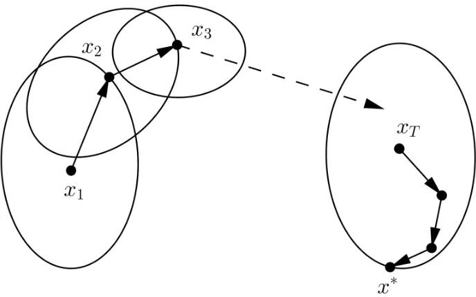
The key idea here is the ellipsoidal view of Newton’s method, whereby we show that after making a constant number of full Newton steps, one can identify an ellipsoid and a norm such that the function is well conditioned with respect to the norm in the ellipsoid. This is depicted in Figure 1.
At this point one can run any desired first-order algorithm. In particular, we choose SVRG and prove its fast convergence. Algorithm 6 (described in the appendix) states the modified SVRG routine for general norms used in Algorithm 5.
We now state and prove the following theorem regarding the convergence of Algorithm 5.
Proof It follows from Lemma 31 that att= f(x1)−f(x∗)
ν , the minimizer is contained in the
Dikin ellipsoid of radiusr, whereν is a constant depending onγ, r. This fact, coupled with Lemma 30, shows that the function satisfies the following property with respect toWxt:
∀x∈Wxt (1−r)
2∇2f(x
T) ∇2f(x)(1−r)−2∇2f(xT).
Using the above fact along with Lemma 32, and substituting for the parameters, concludes the proof.
Figure 1: Visualization of the steps taken in Algorithm 5.
Lemma 30 Letf be a self-concordant function overK, let0< r <1, and considerx∈ K. Let Wr(x) be the Dikin ellipsoid of radius r, and let α= (1−r)2 and β= (1−r)−2. Then,
for all h s.t. x+h∈Wr(x),
α∇2f(x) ∇2f(x+h)β∇2f(x).
Lemma 31 Let f be a self-concordant function over K, let 0 < r < 1, let γ ≥ 1, and consider following the damped Newton step as described in Algorithm 5 with initial point
x1. Then, the number of steps t of the algorithm before the minimizer of f is contained in the Dikin ellipsoid of radius r of the current iterate, i.e. x∗ ∈ Wr(xt), is at most
t= f(x1)−f(x∗)
ν , where ν is a constant depending on γ, r.
Algorithm 5 ellipsoidCover
1: Input : Self-concordantf(x) =
m
P
i=1
fi(x),T,r ∈ {0,1}, initial pointx1∈ K,γ >1,S1, η,T
2: Initialize: xcurr=x1
3: whileλ(xcurr)> 1+rr do
4: step=γ(1 +λ(xcurr))
5: xcurr=xcurr−step1 ∇−2f(xcurr)∇f(xcurr)
6: end while
7: xT+1=N−SVRG(Wr(x), f(x),∇2f(xcurr), S1, η, T)
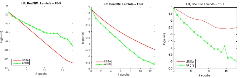
Figure 2: Performance of LiSSA as compared to a variety of related optimization methods for different data sets and choices of regularization parameter λ. S1 = 1, S2 ∼ κln(κ).
Lemma 32 Let f be a convex function. Suppose there exists a convex set K and a positive semidefinite matrix A such that for all x ∈ K, αA ∇2f(x) βA. Then the following
holds between two full gradient steps of Algorithm 6:
E[f(xs)−f(x∗)]≤
1
αη(1−2ηβ)n+
2ηβ (1−2ηβ)
E[f(xs−1)−f(x∗)].
7. Experiments
In this section we present experimental evaluation for our theoretical results.7 We perform the experiments for a classification task over two labels using the logistic regression (LR) objective function with the `2 regularizer. For all of the classification tasks we choose two values ofλ:m1 and 10m, wherem is the number of training examples. We perform the above classification tasks over four data sets: MNIST, CoverType, Mushrooms, and RealSIM. Figure 2 displays the log-error achieved by LiSSA as compared to two standard first-order algorithms, SVRG and SAGA (Johnson and Zhang, 2013; Defazio et al., 2014), in terms of the number of passes over the data. Figure 3 presents the performance of LiSSA as compared to NewSamp (Erdogdu and Montanari, 2015) and standard Newton’s method with respect to both time and iterations.
Figure 3: Convergence of LiSSA over time/iterations for logistic regression with MNIST, as compared to NewSamp and Newton’s method.
7.1 Experiment Details
In this section we describe our experiments and choice of parameters in detail. Table 2 provides details regarding the data sets chosen for the experiments. To make sure our functions are scaled such that the norm of the Hessian is bounded, we scale the above data set points to unit norm.
Table 2: A description of data sets used in the experiments.
Data set m d Reference
MNIST4-9 11791 784 LeCun and Cortes (1998) Mushrooms 8124 112 Lichman (2013) CoverType 100000 54 Blackard and Dean (1999) RealSIM 72309 20958 McCallum (1997)
7.2 Comparison with Standard Algorithms
In Figures 2 and 4 we present comparisons between the efficiency of our algorithm with different standard and popular algorithms. In both cases we plot log(CurrentV alue−
OptimumV alue). We obtained the optimum value for each case by running our algorithm for a long enough time until it converged to the point of machine precision.
Epoch Comparison: In Figure 2, we compare LiSSA with SVRG and SAGA in terms of the accuracy achieved versus the number of passes over the data. To compute the number of passes in SVRG and SAGA, we make sure that the inner stochastic gradient iteration in both the algorithms counts as exactly one pass. This is done because although it accesses gradients at two different points, one of them can be stored from before in both cases. The outer full gradient in SVRG counts as one complete pass over the data. We set the number of inner iterations of SVRG to 2m for the case when λ = 1/m, and we parameter tune the number of inner iterations whenλ= 10/m. The stepsizes for all of the algorithms are parameter tuned by an exhaustive search over the parameters.