Perishability of Data: Dynamic Pricing under Varying-Coefficient Models

Perishability of Data: Dynamic Pricing under

Varying-Coefficient Models

Adel Javanmard [email protected]

Department of Data Sciences and Operations Marshall School of Business

University of Southern California Los Angeles, CA 90089 , USA

Editor:Qiang Liu

Abstract

We consider a firm that sells a large number of products to its customers in an online fashion. Each product is described by a high dimensional feature vector, and the market value of a product is assumed to be linear in the values of its features. Parameters of the valuation model are unknown and can change over time. The firm sequentially observes a product’s features and can use the historical sales data (binary sale/no sale feedbacks) to set the price of current product, with the objective of maximizing the collected revenue. We measure the performance of a dynamic pricing policy via regret, which is the expected revenue loss compared to a clairvoyant that knows the sequence of model parameters in advance.

We propose a pricing policy based on projected stochastic gradient descent (PSGD) and characterize its regret in terms of timeT, features dimensiond, and the temporal variability in the model parameters,δt. We consider two settings. In the first one, feature vectors are chosen antagonistically by nature and we prove that the regret of PSGD pricing policy is of orderO(√T+PT

t=1 √

tδt). In the second setting (referred to as stochastic features model), the feature vectors are drawn independently from an unknown distribution. We show that in this case, the regret of PSGD pricing policy is of orderO(d2logT+PT

t=1tδt/d).

Keywords: Dynamic Pricing, Revenue Management, Varying-Coefficient Models, Regret, Stochastic Gradient Descent, Hypothesis Testing

1. Introduction

Motivated by the prevalence of online marketplaces, we consider the problem of a firm selling a large number of products, that are significantly differentiated from each other, to customers that arrive over time. The firm needs to price the products in a dynamic manner, with the objective of maximizing the expected revenue.

The majority of work in dynamic pricing assume that a retailer sellsidentical items to its customers (Besbes and Zeevi, 2009; Farias and Van Roy, 2010; Broder and Rusmevichien-tong, 2012; den Boer and Zwart, 2013; Wang et al., 2014). Recently, feature-based models have been used to model the products differentiation by assuming that each product is described by vectors of high-dimensional features. These models are suitable for business settings where there are an enormous number of distinct products. One important example is online ad markets. In this context, products are the impressions (user view) that are

c

sold by the web publisher to advertisers. Due to the ever-growing amount of data that is available on the Internet, for each impression there is large number of associated features, including demographic information, browsing history of the user, and context of the web-page. Many other online markets, such as Airbnb, eBay and Etsy also have a similar setting in which products to be sold are highly differentiated. For example, in the case of Aribnb, the products are “stays” and each is characterized by a large number of features including space properties, location, amenities, house rules, as well as arrival dates, events in the area, availability of near-by hotels, etc (Airbnb Documentation, 2015).

Here, we consider a feature-based model that postulates a linear relation between the market value of each product and its feature values. Further, from the firm’s perspective, we treat distinct buyers independently, and hereafter focus on a single buyer. Put it formally, we start with the following model for the buyer’s valuation:

v(xt) =hxt, θi+zt, (1)

wherext∈Rddenotes the product feature vector, θrepresents the buyer’s preferences and

zt,t≥1 are idiosyncratic shocks, referred to as noise, which are drawn independently and

identically from a zero mean distribution. For two vectors a, b, we write ha, bi to refer to their inner product. Feature vectors xt are observable, while model parameterθ is a-priori

unknown to the firm (seller). Therefore, the buyer’s valuationv(xt) is also hidden from the

firm.

Parameters of the above model represents how different features are weighted by the buyer in assessing the product. Considering such model, a firm can use historical sales data to estimate parameters of the valuation model, while concurrently collecting revenue from new sales. In practice, though, the buyer’s valuation of a product will change over time and this raises the concern of perishability of sales data.

In order to capture this point, we consider a richer model with varying coefficients:

vt(xt) =hxt, θti+zt. (2)

Model parametersθtmay change over time and as a result, valuation of a product depends

on both the product feature vector and the time index.

We study a dynamic pricing problem, where at each time periodt, the firm has a product to sell and after observing the product feature vector xt, posts a price pt. If the buyer’s

valuation is above the posted price,vt(xt)≥pt, a sale occurs and the firm collects a revenue

of pt. If the posted price exceeds the buyer’s valuation, pt > vt(xt), no sale occurs. Note

that at each step, the firm has access to the previous feedbacks (sale/no sale) from the buyer and can use this information in setting the current price.

In this paper, we will analyze the varying-coefficient model (2) and answer two funda-mental questions:

First, what is the value of knowing the sequence of model parametersθt; in other

words, what is the expected revenue loss (regret) compared to the clairvoyant policy that knows the parameters of the valuation model in advance? Second, what is a good pricing policy?

from previous feedback on the buyer’s behavior and the problem turns into a random price experimentation. On the other hand, if all of the parameters θt are the same, then this

feedback information can be used to learn the model parameters, which in turn helps in setting the future prices. In this case, an algorithm that performs a good balance between price exploration and best-guess pricing (exploitation) can lead to a small regret. In this work, we study this trade-off through a projected stochastic gradient descent algorithm and investigate the effect of variations of the sequence of θton the regret bounds.

Feature-based models have recently attracted interest in dynamic pricing. (Amin et al., 2014) studied a similar model to (1) (without the noise terms zt), where the features xt

are drawn from an unknown i.i.d distribution. A pricing strategy was proposed based on stochastic gradient descent, which results in a regret of the form O(T2/3√logT). This work also studied the problem of dynamic incentive compatibility in repeated posted-price auctions. Subsequently, (Cohen et al., 2016) studied model (1), wherein the feature vectors

xtare chosen antagonistically by nature and not sampled i.i.d. This work proposes a pricing

policy based on the ellipsoid method from convex optimization (Boyd and Vandenberghe, 2004) with a regret bound ofO(d2log(T /d)), under a low-noise setting. More accurately, the regret scales asO(d2log(min{T /d,1/δ}) +dδT), whereδ measures the noise magnitude: in case of bounded noise,δ represents the uniform bound on noise and in case of gaussian noise with varianceσ2, it is defined as δ= 2σplog(T). In (Lobel et al., 2016), the regret bound of this policy was improved to O(dlogT), under the noiseless setting. In (Javanmard and Nazerzadeh, 2016), authors study and highlight the role of the structure of demand curve in dynamic pricing. They introduce model (1), and assume that the feature vectors xt are

drawn i.i.d. from an unknown distribution. Further, motivated by real-world applications, it is assumed that the parameter vectorθis sparse in the sense that only a few of its entries are nonzero. A regularized log-likelihood approach is taken to get an improved regret bound of orders0(log(d) + log(T)). We add to this body of work by considering feature-based models for valuation of products whose parameters vary over time.

Time-varying demand environments have also been studied recently by (Keskin and Zeevi, 2016). Explicitly, they consider a firm that sells one type of product to customers that arrive over a time horizon. After setting price pt, the firm observes demand Dt given

byDt=αt+βtpt+t, whereαt, βt∈Rare the unknown parameters of the demand model and t are the unobserved demand shocks (noise). By contrast, in this work we consider

different products, each characterized by a high-dimensional feature vector. Further, the seller only receives a binary feedback (sale/no sale) of the customer’s behavior at each step, rather than observing the customer’s valuation.

1.1 Organization of paper and our main contributions

The remainder of this paper is structured as follows. In Section 2, we formally define the model and formulate the problem. Technical assumptions and the notion of regret will be discussed in this section. We next propose a pricing policy based on projected stochastic gradient descent (PSGD) applied to the log-likelihood function. At each time period t, it returns an estimate θb_t. The price p_t is then set to the optimal price as ifθb_t was the actual

parameter θt. We next analyze the regret of our PSGD algorithm. Let δt = kθt+1 −θtk

setting where the product feature vectors xt are chosen antagonistically by nature and

show that the regret of PSGD algorithm is of order O(√T +PT_t=1√tδt). Interestingly,

this bound is independent of the dimension d, which is a desirable property of our policy for high-dimensional applications. We next, in Section 4, consider a stochastic features model, where the feature vectorsxtare drawn independently from an unknown distribution

(cf. Assumption 6). Under this setting, we show that the regret of PSGD is of order

O(d2logT+PT_t=1tδt/d). Note that settingδt= 0 corresponds to model (1) and our PSGD

pricing obtains a logarithmic regret inT. Section 7 is devoted to the proof of main theorems and the main lemmas are proved in Section 8. Finally, proof of several technical steps are deferred to Appendices.

1.2 Related literature

Our works is at the intersection of dynamic pricing, online optimization and high-dimensional statistics. In the following, we briefly discuss the work most related to ours from these con-texts.

Feature-based dynamic pricing. Recent papers on dynamic pricing consider models with features/covariates, motivated in part by new advances in big data technology that allow firms to collect large amount of fine-grained information. In the introduction, we discussed the work (Amin et al., 2014; Javanmard and Nazerzadeh, 2016; Cohen et al., 2016) which are closely related to our setting. Another recent work on feature-based dynamic pricing is (Qiang and Bayati, 2016). In this work, authors consider a model where the seller observes the demand entirely, rather than a binary feedback as in our setting. A greedy iterative least squares (GILS) algorithm is proposed that at each time period estimates the demand as a linear function of price by applying least squares to the set of prior prices and realized demands. The work underscores the role of feature-based approaches and show that they create enough price dispersion to achieve a regret of O(log(T)). This is closely related to the work of (den Boer and Zwart, 2013) and (Keskin and Zeevi, 2014) in dynamic pricing (without demand covariates) that demonstrate the GILS is suboptimal and propose methods to integrate forced price-dispersion with GILS to achieve optimal regret.

Online optimization. This field offers a variety of tools for sequential prediction, where an agent measures its predictive performance according to a series of convex functions. Specifically, there is a sequence of a priori unknown reward functions f1, f2, f3, . . . and an agent must make a sequence of decisions: at each time period t, he selects a point zt and

a lossft(zt) is incurred. Note that the function ft is not known to agent at stept, but he

has access to all previous functions f1, . . . , ft−1. First order methods, like online gradient descent (OGD) or online mirror descent (OMD) only use the gradient of previous function at the selected points, i.e., ∂ft(zt). The notion of regret here is defined by comparing the

agent with the best fixed comparator (Shalev-Shwartz, 2011).

(Hall and Willett, 2015) proposed dynamic mirror descent that is capable of adapting adapts to a possibly non-stationary environment. In contrast to OMD (Beck and Teboulle, 2003; Shalev-Shwartz, 2011), the notion of regret is defined more generally with respect to the best comparator “sequence”.

in time periodt, i.e.,ft=−ptI(pt≥vt). Then (i) the loss functions are not convex; (ii) the

(first order information) of previous loss functions depend on the corresponding valuations

v1, . . . , vt−1 which are never revealed to the seller. That said, we borrow some of the techniques from online optimization in proving our results. (See proof of Lemma 3.)

High-dimensional statistics. Among the work in this area, perhaps the most related one to our setting is the problem of 1-bit compressed sensing (Plan and Vershynin, 2013a,b; Ai et al., 2014; Bhaskar and Javanmard, 2015). In this problem, a set of linear measurements are taken from an unknown vector and the goal is to recover this vector having access to the sign of these measurements (1-bit information). This is related to the dynamic pricing problem on model (1), as the seller observes 1-bit feedback (sale/no sale from previous time periods). However, there are a few important differences between these two problem that are worth noting: 1) In dynamic pricing, the crux of the matter is the decisions (prices) made by the firm. Of course this task entails learning the model parameters and therefore the firm gets into the realm of exploration (learning) and exploitation (earning revenue). By contrast, 1-bit compressed sensing is only a learning task; 2) In dynamic pricing, the prices are set based on the previous (sale/no sale) feedbacks. Therefore, the feedbacks are inherently correlated and this makes the learning task challenging. However, in 1-bit compressed sensing it is assumed that the measurements (and therefore the observed signs ) are independent; 3) The majority of work on 1-bit compressed sensing consider an offline setting, while in the dynamic pricing, decision are made in an online manner.

2. Model

We consider a pricing problem faced by a firm that sells products in a sequential manner. At each time period t = 1,2,· · ·, T the firm has a product to sell and the product is represented by anobservablevector of features (covariates)xt∈ X ⊆Rd. The length of the time horizon, denoted by T, is unknown the to the firm and the setX is bounded.

The product at timethas a market valuevt=vt(xt), depending on bothtandxt, which

isunobservable. At each periodt, the firm (seller) posts a pricept. Ifpt≤vt, a sale occurs,

and the firm collects revenuept. If the price is set higher than the market value,pt> vt, no

sale occurs and no revenue is generated. The goal of the firm is to design a pricing policy that maximizes the collected revenue.

We assume that the market value of a product is a linear function of its covariates, namely

vt(xt) =hθt, xti+zt. (3)

Here,θtandxtared-dimensional and{zt}t≥1 are idiosyncratic shocks, referred to as noise, which are drawn independently and identically from a zero-mean distribution over R. We denote its cumulative distribution function byF, and the corresponding density byf(x) =

F0(x). Note that the noise can account for the features that are not measured. We refer to (Keskin and Zeevi, 2014; den Boer and Zwart, 2014; Qiang and Bayati, 2016) for a similar notion of demand shocks.

The regret is measured with respect to the clairvoyant policy that knows the sequence θin advance. We will formally define the regret in Section 2.2.

Let yt be the response variable that indicates whether a sale has occurred at periodt:

yt= (

+1 ifvt≥pt,

−1 ifvt< pt.

(4)

Note that the above model foryt can be represented as the following probabilistic model:

yt= (

+1 with probability 1−F(pt− hθt, xti)

−1 with probability F(pt− hθt, xti)

(5)

2.1 Technical assumptions and notations

For a vectorv, we writekvkpfor the standard`pnorm of a vectorv, i.e.,kvkp= (P_i|vi|p)1/p.

Whenever the subscript p is not mentioned it is deemed as the `2 norm. For a matrix A,

kAk denotes its `2 operator norm. For two vectors a, b, we use the notation ha, bi to refer to their inner product.

To simplify the presentation, we assume that kxtk ≤1, for all xt ∈ X, and kθtk ≤W

for a known constant W. We denote by Θ the d-dimensional `2 ball of radius W (In fact, we can take Θ to be any convex set that contains parameters θt. The size of Θ effects our

regret bounds up to a constant factor.)

We also make the following assumption on the distribution of noise F.

Assumption 1 The function F(v) is strictly increasing. Further, F(v) and 1−F(v) are log-concave inv.

Log-concavity is a widely-used assumption in the economics literature (Bagnoli and Bergstrom, 2005). Note that if the density f is symmetric and the distribution F is log-concave, then 1−F is also log-concave. Assumption 1 is satisfied by several common proba-bility distributions including normal, uniform, Laplace, exponential, and logistic. Note that the cumulative distribution function of all log-concave densities is also log-concave (Boyd and Vandenberghe, 2004).

We use the standard big-O notation. In particular f(n) = O(g(n)) if there exists a constantC >0 such that |f(n)| ≤Cg(n) for alln large enough. We also use R≥0 to refer to the set of non-negative real-valued numbers.

2.2 Benchmark policy and regret minimization

For a pricing policy, we measures its performance via the notion of regret, which is the expected revenue loss compared to an oracle that knows the sequence of model parameters in advance (but not the realizations of{zt}t≥1).We first characterize this benchmark policy. Using Eq. (3), the expected revenue from a posted price p is equal to p×_P(vt ≥p) =

p(1−F(p−θt·xt)). First order condition for the optimal pricep∗(xt, θt) reads

p∗(xt, θt) =

1−F(p∗(xt, θt)− hθt, xti)

f(p∗_(x

t, θt)− hθt, xti)

To lighten the notation, we drop the arguments xt, θt and denote by p∗t the optimal price

at timet.

We next recall thevirtual valuation function, commonly used in mechanism design (My-erson, 1981):

ϕ(v)≡v−1−F(v)

f(v) .

Writing Eq. (6) in terms of function ϕ, we get

hθt, xti+ϕ(p∗t− hθt, xti) = 0.

In order to solve forp∗_t, we define the pricing functiong as follows:

g(v)≡v+ϕ−1(−v). (7)

By Assumption 1, ϕ is injective and hence g is well-defined. Further, it is easy to verify thatg is non-negative. Using the definition of g and rearranging the terms we obtain

p∗_t =g(hθt, xti). (8)

The performance metric we use in this paper is the worst-case regret with respect to a clairvoyant policy that knows the sequenceθ in advance. Formally, for a policyπ to be the seller’s policy that sets pricept at period t, the worst-case regret is defined over T periods

is defined as:

Regretπ(T)≡sup∆π_θ,x : θt∈Θ, xt∈ X , (9)

where forT ≥1,θ= (θ1, . . . , θT) andx= (x1, x2, . . . , xT),

∆π_θ,x(T) =Eθ,x " _T

X

t=1

p∗_tI(vt≥p∗t)−ptI(vt≥pt)

#

. (10)

Here the expectationEθ,x is with respect to the distributions of idiosyncratic noise,zt. Note

thatvt,pt, and p∗t depend onθ andx.

3. Pricing policy

Our dynamic pricing policy consists of a projected gradient descent algorithm to predict parameters θb_t. With each new product, it computes the negative gradient of the loss and

shirts its prediction in that direction. The result is projected onto set Θ to produce the next prediction. The policy then sets the prices as pt =g(hxt,θb_ti). Note that by Eq. (7),

pt is the optimal price if θb_t was the true parameterθ_t. Also, by log-concavity assumption

on F and 1−F, the function`t(θ) is convex.

PSGD (Projected stochastic gradient descent) pricing policy Input: (at time 0)functiong, set Θ,

Input: (arrives over time) covariate vectors{xt}t∈N

Output: prices{pt}t∈_N

1: p1 ←0 and initializeθb₁ ∈Θ

2: fort= 1,2,3, . . . do

3: Setθb_t+1 according to the following rule: b

θt+1 = ΠΘ(θb_t−η_t∇`_t(θb_t)) (11)

with

`t(θ) =−I(yt= 1) log(1−F(pt− hxt, θi))−I(yt=−1) log(F(pt− hxt, θi)) (12)

4: Set pricept+1 as

pt+1←g(hxt+1,θb_t+1i) (13)

3.1 Regret analysis

We first define a few useful quantities that appear in our regret bounds. Define

M ≡ W +ϕ−1(0), (14)

uM ≡ sup

|x|≤M

maxn− d

dxlogF(x),−

d

dxlog(1−F(x))

o

, (15)

`M ≡ inf

|x|≤M

minn− d

2

dx2logF(x),− d2

dx2 log(1−F(x))

o

, (16)

where the derivatives are with respect to x. We note that M is an upper-bound on the maximum price offered and also, by the log-concavity property ofF and 1−F, we have

uM = max n

− d

dxlogF(−M),−

d

dxlog(1−F(M))

o

.

Further, by log-concavity property ofF and 1−F, we have `M >0.

We also let B = maxvf(v) and B0 = maxvf0(v), respectively denote the maximum

value of the density function f and the its derivative f0.

The following theorem bounds the regret of our PSGD policy.

Theorem 2 Consider model (3) for the product market values and let Assumption 1 hold. Set M = 2W +ϕ−1(0), with ϕ being the virtual valuation function w.r.t distribution F. Then, the regret of PSGD pricing policy using a non-increasing sequence of step sizes{ηt}t≥1 is bounded as follows:

Regret(T)≤ 2(2B+M B

0₎

`M

max

16

`M

logT, 2W

2

ηT+1 +u

2

M

2

T X

t=1

ηt+ 2W T X

t=1

δt

ηt

+M

T , (17)

In particular, if ηt ∝ √1_t, then there exists a constant C = C(B, M, W, `M, uM) > 0,

independent ofT, such that

Regret(T)≤C

√ T+ T X t=1 √ tδt . (18)

At the core of our regret analysis (proof of Theorem 2) is the following Lemma that provides a prediction error bound for the customer’s valuations.

Lemma 3 Consider model (3) for the product market values and let Assumption 1 hold. Set M = 2W +ϕ−1(0), with ϕ being the virtual valuation function w.r.t distribution F. Let {θb_t}_t≥1 be generated by PSGC pricing policy, using a non-increasing positive series

ηt+1≤ηt. Then, with probability at least1−_T12 the following holds true:

T X

t=1

hxt, θt−θb_ti2 ≤

4 `M max 16 `M logT,

2W2 η1 + T X t=1 1

2ηt+1

− 1

2ηt

kθt+1−θb_t+1k2+

u2_M

2

T X

t=1

ηt+ 2W T X t=1 δt ηt , (19)

where uM, `M are given by Equations (15),(16), respectively.

Lemma 3 is presented in a form that can also be used in proving our next results under the stochastic features model. For proving Theorem 2, we simplify bound (19) as follows. Given thatθt+1,θb_t+1 ∈Θ, we havekθ_t+1−θb_t+1k ≤2W. Using the non-increasing property

of sequenceηt, we write

2W2 η1 + T X t=1 1 2ηt+1

− 1

2ηt

kθt+1−θb_t+1k2≤

2W2 η1 + T X t=1

2W2 ηt+1

−2W

2

ηt

≤ 2W

2

ηT+1

.

Therefore, bound (19) simplifies to:

T X

t=1

hxt, θt−θb_ti2 ≤

4 `M max 16 `M

logT, 2W

2

ηT+1 +u 2 M 2 T X t=1

ηt+ 2W T X t=1 δt ηt , (20)

The regret bound (17) is derived by relating regret at each time period to the prediction error at that time. We refer to Section 7 for the proof of Theorem 2.

Remark 4 The regret bound (17) does not depend on the dimension d, which makes our pricing policy desirable for high-dimensional applications. Also, note that the temporal variation δt appears in our bound with coefficient

√

Remark 5 While the regret bound is dimension-free, the computational complexity of PSGD pricing policy scales with dimensiond. Specifically, the complexity of each step is O(d). To see this, we note that the gradient ∇`t(θ) can be computed in O(d) by Equations (70)

and (71). Projection onto setΘ (`2 projection) is alsoO(d). 4. Stochastic features model

In Theorem 2, we showed that our PSGD pricing policy achieves regret of order O(√T +

PT t=1

√

tδt). Let us point out that in Theorem 2 the arrivals (feature vectorsxt) are modeled

as adversarial. In this section, we assume that featuresxt are independent and identically

distributed according to a probability distribution onRd. Under such stochastic model, we show that the regret of PSGD pricing scales at most of orderO(d2logT +PT_t=1tδt/d).

We proceed by formally defining the stochastic features model.

Assumption 6 (Stochastic features model). Feature vectors xt are generated

indepen-dently according to a probability distribution Px, with a bounded support inRd. We denote by Σ the covariance matrix of distribution Px and assume that Σhas bounded eigenvalues.

Specifically, there exist constants Cmin and Cmax such that for every eigenvalue σ of Σ, we have 0< _d1Cmin ≤σ < 1_dCmax.

Without loss of generality and to simplify the presentation, we assume that Px is

sup-ported on the unit`2 ball inRd. The rationale behind the above assumption on the scaling of eigenvalues is that Trace(Σ) = E(kxtk2) ≤ 1. Therefore, the assumption above on the

eigenvalues of Σ states that all the eigenvalues are of the same order.

Under the stochastic features model, we define the notion of worst-case regret as follows. For a policy π be the seller’s policy that sets price pt at period t, the T-period regret is

defined as:

Regretπ(T)≡sup∆π_θ,Px : θt∈Θ,Px ∈Q , (21)

where Q denotes the set of probability distribution supported on `2 unit ball satisfying Assumption 6 (bounded eigenvalues). Further, for T ≥1,θ = (θ1, . . . , θT) and probability

measure Px, we define

∆π_θ,Px(T) =Eθ,Px

" _T

X

t=1

p∗_tI(vt≥p∗t)−ptI(vt≥pt)

#

. (22)

where the expectation is with respect to the distributions of idiosyncratic noise,zt, andPx,

the distribution of feature vectors. Note the subtle difference with definition (9), in that the worst case is computed overQrather than X.

We propose a similar PSGD pricing policy for this setting, with a specific choice of the step sizes. Ideally, we want to setηt= 6/(`MCt), whereCis an arbitrary fixed constant such

that 0< C < σmin, withσminbeing the minimum eigenvalue of population covariance Σ. Of course, Σ is unknown and therefore we proceed as follows. We letQt= (1/t)Pt`=1x`xT` be

the empirical covariance based on the firsttfeatures. Denote byσtthe minimum eigenvalue

of Qt. We then use the sequenceσt, and set the step sizeηt as

ηt=

1

λt·t

, λt=

`M

6

(

1

t

1 +

t X

`=1

σ`

)

PSGD pricing policy for stochastic features model Input: (at time 0)functiong, set Θ,

Input: (arrives over time) covariate vectors{xt}t∈_N Output: prices{pt}t∈_N

1: p1 ←0 and initializeθb₁ ∈Θ

2: Q1←x1xT1

3: fort= 1,2,3, . . . do

4: Define σt as the minimum eigenvalue ofQt.

5: Set

λt=

`M

6t(1 +

t X

`=1

σ`). (23)

6: Set

ηt=

1

λt·t

(24)

7: Setθb_t+1 according to the following rule: b

θt+1 = ΠΘ(θb_t−η_t∇`_t(θb_t)) (25)

with

`t(θ) =−I(yt= 1) log(1−F(pt− hxt, θi))−I(yt=−1) log(F(pt− hxt, θi)) (26)

8: Qt+1←(_t+1t )Qt+ (_t+11 )xt+1xTt+1 9: Set pricept+1 as

pt+1←g(hxt+1,θb_t+1i) (27)

Description of the PSGD pricing policy is given in Table above.

4.1 Logarithmic regret bound

The following theorem bounds the regret of our dynamics pricing policy.

Theorem 7 Consider model (3) for the product market values and suppose Assumption 1 holds. LetM = 2W +ϕ−1(0), with ϕbeing the virtual valuation function w.r.t distribution

F. Under the stochastic features model (Assumption 6), the regret of PSGD pricing policy is bounded as follows:

Regret(T)≤C1d2logT +C2

T X

t=1

t

whereδt≡ kθt+1−θtkandC1, C2are constants that depend onCmax, Cmin, uM, `M, M, B, W

but are independent of dimension d.

Proof of Theorem 7 relies on the following lemma that is analogous to Lemma 3 and estab-lishes a prediction error bound for the customer’s valuations.

Lemma 8 Consider model (3) for the product market values and the stochastic features model (Assumption 6). Suppose that Assumption 1 holds and set M = 2W +ϕ−1(0), with

ϕ being the virtual valuation function w.r.t distribution F. Let {θb_t}_t≥1 be generated by PSGD pricing policy. Then,

Cmin

T X

t=1

E(kθt−θb_tk2)≤

128

`2_M +

24u2_M `2_M

˜

c+ 4

Cmind

·d3logT

+ 8W2d

1

T +

12

`2

M

+ 1

c2d

+ 4W

T X

t=1

tδt.

Here σmin denotes the minimum eigenvalue of covariance Σ. (See Assumption 6.) 4.2 A lower bound on regret

In this section, we provide a theoretical lower bound on the minimum achievable regret of any pricing policy under the stochastic features model. Prior to that, we need to adopt a few notations.

For a given time horizon T and a sequence of valuations parameters θ = (θ1, . . . , θT),

let

Vθ(T)≡ T X

t=1

tkθt+1−θtk. (29)

We also define, for ν ∈[1/2,2],

V(T, B, ν)≡ {θ: θt∈Θ, Vθ(T)≤BdTν}. (30)

By assuming θ ∈ V(T, B, ν) for all T, we are assuming that nature has a finite temporal variation budget to use in changing the valuation parameters throughout the time horizon. Of course, different variation metrics can be considered such as total variation PT_t=1δt

or the maximum temporal variation sup1≤t≤Tδt and the performance of a pricing policy

changes, the policy can be designed in a way to detect the changes and reset its estimate of the valuation model after each change to avoid large estimation error and revenue loss. For a pricing policy π, consider theT-period regret, defined as

Regretπ(T, B, ν)≡maxn∆π_θ,Px(T) : θ ∈ V(T, B, ν),Px ∈Q

o

(31)

where we recall that

∆π_θ,Px(T)≡

T X

t=1 Eθ,Px

p∗_tI(vt≥p∗t)−ptI(vt≥pt)

. (32)

Note that this is the same regret notion defined in (21), where we just make the variation budget constraint explicit in the notation.

Rephrasing the statement of Theorem 7, for PSGD pricing policy we haveRegretπ(T, B, ν)≤

C1d2logT +C2BTν. We next provide a lower bound on the regret of any pricing policy. Indeed this lower bound applies to a powerful clairvoyant who fully observes the market values after the price is either accepted or rejected.

Theorem 9 Consider linear model (3) where the market values vt(xt), 1 ≤ t ≤ T, are

fully observed. We further assume that market value noises are generated aszt∼N(0, σ2).

There exists a constant c, depending on σ, Cmax, such that

Regretπ(T, B, ν)≥cmin B2dT2ν−11/3, T /d,

for any pricing policy π and time horizon T.

The high-level intuition behind this result is that the nature can change the valuation parameters in a gradual manner such that the seller should pay a revenue loss in order to detect the changes and learn the new valuation parameter after a change. To be more specific, we divide the time horizon into cycles of length N periods, where N is of order (T4−2ν/d)1/3 and consider a setting where the value ofθtcan change to one of two options

θ0, θ1, only in the first period of a cycle. We choose the parameter change δ =kθ1−θ0k of order pd/N to ensure that (i) no policy can identify the change without incurring a revenue loss of order N δ2/d (ii) The variation metric Vθ(T) remains below the allowable

limit ofBdTν. Therefore, the total regret overT periods works out atT δ2/d. In particular, for proving point (i) we quantify the likelihood of valuations under the probability measures corresponding to θ0 and θ1, using Kullback-Leibler divergence. We use Pinsker inequality form probability theory and hypothesis testing results from information theory to show that there is a significant probability of not detecting the (potential) change, which consequently yields a revenue loss of order N δ2/d, over each cycle.

We refer to Section 7.3 for the proof of Theorem 9.

5. Numerical experiments

We numerically study the performance of our PSGD pricing policy on synthetic data. In our experiments, we set W = 5 and set θ1 = (W/2)(Z/kZk), with Z ∼N(0,Id) a multivariate

normal variable. We then generate a sequence of parametersθt as follows:

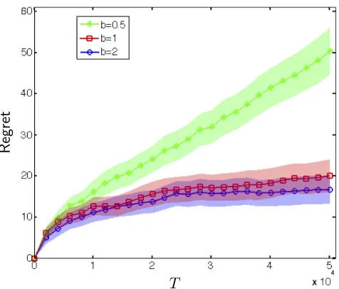
T

Regret

Figure 1: Cumulative regret of PSGD pricing policy for the synthetic data in Section 5. Temporal variations are δt=t−b and the curves are obtained by averaging across 80 trials.

Shaded region around each curve is the 95% confidence interval.

wherert=t−b( ˜Z/kZ˜k), with ˜Z ∼N(0,Id). Note thatδt=kθt+1−θtk=krtk=t−b.

Next, at each time t, product covariatesxtare independently sampled from a Gaussian

distribution N(0,Id) and normalized so that kxtk = 1. Further, the market shocks are

generated as zt ∼ N(0, σ2), with σ = 1. We run the PSGD pricing policy for stochastic

features model.

Results. Figure 1 compares the cumulative regret (averaged over 80 trials) of the PSGD policy, for b = 0.5,1,2, on the aforementioned synthetic data for T = 50,000 steps. The shaded region around each curve correspond to the 95% confidence interval across the 80 trials. As expected, increase inb results in larger temporal variations and larger regret.

To better understand the behavior of regret for different values ofb, we plotted the regret bounds in various scales in Figure 2. Forb= 0.5, we haveRegret(T)∼T2/3, and forb= 1,2, we have Regret ∼ log(T). Comparing with Theorem 7, we see that the empirical regret in case of b= 0.5, 1, is smaller than the upper bound given by Equation (28), order-wise. However, it is worth noting that bound given in Theorem 7 applies to any adversarial choice of temporal variationsrt, while in our experiments we generated these terms independently

at random.

6. Extension to nonlinear model

Throughout the paper, we exclusively focused on linear models for buyer’s valuation with varying coefficients. In order to generalize our results to nonlinear models, we consider a setting where the market value of a product with feature vectorxt is given by

7.5 8 8.5 9 9.5 10 10.5 11 1.5

2 2.5 3 3.5 4

log(T)

log

(

Regret

)

(a)b= 0.5

7.5 8 8.5 9 9.5 10 10.5 11 6

8 10 12 14 16 18 20 22

log(T)

Regret

(b) b= 1

7.5 8 8.5 9 9.5 10 10.5 11 4

6 8 10 12 14 16 18

log(T)

Regret

(c) b= 2

Figure 2: Cumulative regrets of PSGD for different values of b. For b= 0.5, Regret(T) ∼

This model is often referred to as generalized linear model and captures nonlinear depen-dencies on features to some extent. We assume that the link functionψ:R7→Ris a general log-concave function and is strictly increasing.

We next compute the pricing function. Since ψ is strictly increasing, the expected revenue at a pricep amounts to p 1−F ψ−1(p)− hxt, θti

. First order condition for the optimal pricep∗_t(xt) reads as

ψ0(ψ−1(p∗_t)) = pf ψ −1_(p∗

t)− hxt, θti

1−F(ψ−1_(p∗

t)− hxt, θti)

. (34)

Define λ(v) = f(v)/(1−F(v)) the hazard rate function for distribution F, and let ˜p =

ψ−1(p). Writing (34) in terms ofλfunction, we get

hxt, θti= ˜p∗t −λ

−1

ψ0(˜p∗_t)

ψ(˜p∗_t)

. (35)

For real-valued v, define

g−1_ψ (v)≡v−λ−1

ψ0(v)

ψ(v)

. (36)

Note that by log-concavity of 1−F, the hazard function λ is increasing. Also, by log-concavity of ψ, the term _dd_vlogψ(v) = ψ0(v)/ψ(v) is decreasing. Putting these together, we obtain that −λ−1(ψ0(v)/ψ(v)) is increasing. Therefore, the right-hand side of (36) is strictly increasing and the function gψ is well-defined. Invoking Equation (35), we derive

the optimal price as

p∗_t =ψ(gψ(hxt, θti)). (37)

As noted before, since ψ is increasing, at each period t, a sale happens if zt ≥ ψ−1(pt)−

hxt, θti. Hence, the log-likelihood function reads as

`t(θ) =−I(yt= 1) log 1−F ψ−1(pt)− hxt, θi

−_I(yt=−1) log F ψ−1(pt)− hxt, θi

.

(38)

In PSGD pricing policy, we run gradient step with this log-likelihood function and then set pricept+1 at next step as pt+1=ψ(gψ(hxt+1, θt+1i)).

The results on the regret of PSGD pricing policy carries over to the generalized linear model as well. The analysis goes along the same lines and is omitted.

7. Proof of main theorems

7.1 Proof of Theorem 2

Lemma 10 Set M = 2W +ϕ−1(0), and for θ ∈ Θ define ut(θ) = pt− hxt, θi, where

pt=g(hxt,θb_ti) is the posted price at time t. Then |u_t(θ)| ≤M for all t≥1.

Define function h(;u) from R≥0 toR≥0 as

This is the expected revenue at price p when the noiseless valuation is u, i.e.,hxt, θti=u.

We let

Rt≡p∗tI(vt≥pt∗)−ptI(vt≥pt) (39)

be the regret incurred at time t, and defineFt as the history up to timet (Formally,Ft is

theσ-algebra generated by market noise {z`}t`=1.) Then,

E(Rt|Ft−1) =p∗tP(vt≥p∗t)−ptP(vt≥pt) =h(p∗t;hxt, θti)−h(pt;hxt,θb_ti). (40)

The optimal price p∗_t is the maximizer of h(p;hxt, θti) and thus h0(p∗t;hxt, θti) = 0. By

Taylor expansion of functionh, there exists a valuepbetweenptand p∗t, such that,

h(pt;hxt, θti)−h(p∗t;hxt, θti) =

1 2h

00

(p;hxt, θti)(pt−p∗t)2. (41)

We next show that|h00(p;hxt, θti)| ≤C withC= 2B+M B0. Recall thatB = maxvf(v)

and B0 = maxvf0(v). To see this, we write

|h00(p;hxt, θti)|=

2f(p− hxt, θti) +pf

0_{(p− hx}

t, θti)

≤2B+M B

0_{. (42)}

Putting Equations (39), (41), (42) and using the 1-Lipschitz property of price function g, we conclude:

E[Rt|Ft−1] =h(p∗t;hxt, θti)−h(pt;hxt,bθ_ti)≤

2B+M B0

2 (pt−p ∗

t)2

= 2B+M B 0

2

g(hxt,θb_ti)−g(hx_t, θ_ti) 2

≤ 2B+M B

0

2 hxt, θt−θbti

2 ₍₄₃₎ To ease the presentation, define the shorthand

A(T)≡ 4

`M

max

16

`M

logT, 2W

2

ηT+1 +u

2

M

2

T X

t=1

ηt+ 2W T X

t=1

δt

ηt

.

We further let G be the probabilistic event that PT_t=1hxt, θt−θb_ti2 ≤ A(T). Employing

Lemma 3 and using the fact that kθt+1−θb_t+1k2 ≤4W2, we obtain that P(G)≥1−_T12. We continue by bounding E(Rt) as follows:

E[Rt] =E[E[Rt|Ft−1]] =E

h

E[Rt|Ft−1]·

I(G) +I(Gc)

i

= 2B+M B 0

2 E

h

hxt, θt−bθ_ti2·_I(G) i

+MP(Gc).

Consequently,

Regret(T)≤

T X

t=1

E[Rt]≤

2B+M B0

2 E

hXT

t=1

hxt, θt−bθ_ti2·I(G) i

+M T P(Gc)≤ 2B+M B 0

2 A(T) +

M T .

7.2 Proof of Theorem 7

Proof of Theorem 7 follows along the same lines as proof of Theorem 2. Let ˜Ft be the

σ-algebra generated by market noises {z`}t`=1 and feature vectors {x`}t`=1. Further, let Ft

be the σ-algebra generated by ˜F_t∪ {xt+1}. For term Rt defined by (39) and following the

chain of inequalities as in (43),

E[Rt|Ft−1]≤

2B+M B0

2 hxt, θt−θbti

2_{. (44)}

For brevity in notation, let ¯B = (2B+M B0)/2. Since,Ft⊇F˜t, by iterated law of iteration,

E(Rt|F˜t−1) =E(E(Rt|Ft−1)|F˜t−1)≤B¯hθt−θb_t,Σ(θ_t−θb_t)i ≤

1

d

¯

BCmaxkθt−θb_tk2 (45)

Applying Lemma 8, we get

Regret(T)≤

T X

t=1

E[Rt]≤

1

dBC¯ max

T X

t=1

E(kθt−θb_tk2)

≤B¯Cmax Cmin

128

`2

M

+24u 2

M

`2

M

˜

c+ 4

Cmind

·d2logT

+ 8W2B¯Cmax Cmin

1

T +

12

`2_M +

1

c2d

+ ¯BCmax Cmin

4W

d

_XT

t=1

tδt.

The result follows by taking

C1 = ¯B

Cmax

Cmin

8W2

1

T +

12

`2_M +

1

c2d

+128

`2_M +

24u2_M `2_M

˜

c+ 4

Cmind

,

C2 = 4WB¯

Cmax

Cmin

.

7.3 Proof of Theorem 9

The proof methodology is similar to the proof of (Keskin and Zeevi, 2016, Theorem 1). We first propose a setting for constructing the sequence of valuation parameters θ = (θ1, . . . , θT). Divide the time horizon into cycles of lengthN =dm0T(4−2ν)/3e, wherem0= (_C σ2

maxB2d)

1/3_{. Consider a setting wherein the noise markets are generated as z}

t∼N(0, σ2)

and the value of θt can change only in the first period of a cycle, taking one of the two

values {θ0, θ1}. Here, θ0, θ1 ∈Rd are two arbitrary vectors such that kθ0−θ1k =δ, with

δ= min(σpd/(CmaxN),

√

c2). Note that for this sequence of θ, we have

Vθ(T)≤

dT /Ne

X

k=1

(kN)δ ≤ T

2

N δ≤BdT

ν ₍₄₆₎

We consider a clairvoyant who fully observes the market values vt(xt). Focus on a single

when all the parameters θt are equal to θ0 (resp. θ1), for 1≤t ≤N. The KL divergence

betweenPπ0 and Pπ1 amounts to

DKL(Pπ0,Pπ1)≡Eπ0log



  

QN t=1φ

vt− hxt, θ0i

σ

QN t=1φ

vt− hxt, θ1i

σ



  

. (47)

whereEπ0 denotes expectation w.r.tPπ0 andφ(s) = 1/(

√

2π)e−s2/2 is the standard Gaussian density. After simple algebraic manipulation, we obtain

DKL(Pπ0,Pπ1) =− 1 2σ2E

π

0

N

X

t=1

(2zt− hxt, θ1−θ0i)hxt, θ1−θ0i

= 1

2σ2

N X

t=1

Eπ0(hxt, θ1−θ0i2)≤

1 2σ2_d

N X

t=1

Cmaxkθ1−θ0k2

= 1

2σ2Cmax

δ2N d .

We next relate the expected regret to the KL divergence betweenPπ0 and Pπ1.

Lemma 11 Let Rt be the regret incurred at timet, defined as Rt≡p∗tI(vt≥p∗t)−ptI(vt≥

pt). Then, there exist constants c1, c2 depending on σ, W, andCmin, such that

E(Rt)≥

c1

dE

n

min

kθb_t−θ_tk2₂, c₂ o

. (48)

Proof of Lemma 11 goes along the proof of (Javanmard and Nazerzadeh, 2016, Equation (55)) and is omitted.

By applying Lemma 11, we have

∆π_θ,Px(N) =

N X

t=1

Eθ(Rt)≥

c1

d

N X

t=1 E

n

min

kθb_t−θ_tk2₂, c₂ o

. (49)

For brevity in notations, for the sequenceθ= (θ1, . . . , θN), we defineda(θ) =c1PN_t=1min(kθt−

θak2

2, c2), for a= 1,2. Define two setsJa, fora= 1,2 as follows:

Ja=

θ= (θ1, . . . , θN) : θi ∈Rd,da(θ)<

1 4N δ

2

. (50)

max ∆π_0,Px(N),∆π_1,Px(N)≥ 1

dmax

Eπ0(d0(θ)),Eπ1(d1(θ))

≥ N

4dδ

2_max

Pπ0(θ∈/J0),Pπ1(θ∈/ J1)

(a)

≥ N

4dδ

2_max

Pπ0(θ ∈/ J0),Pπ1(θ∈J0)

≥ N

8dδ

2

Pπ0(θ∈/J0) +Pπ1(θ∈J0)

≥ N

8dδ

2₁₋

Pπ0(θ∈J0) +Pπ1(θ∈J0)

≥ N

8dδ

2₁₋

r

1

2DKL(P

π

0,Pπ1)

(By Pinsker inequality)

≥ N

8dδ

2 ₁₋ 1 2σδ

r

Cmax

N d

!

≥ N δ

2 16d .

Here (a) holds because θ ∈ J0 implies θ ∈/ J1. Otherwise, d0(θ) < N δ2/4 and d1(θ) <

N δ2/4. Using the inequality min(a+b, c) ≤ min(a, c) + min(b, c) for a, b, c ≥ 0, and applying triangle inequality, we get

Nmin(kθ0−θ1k2, c2)≤2d0(θ) + 2d1(θ)< N δ2, (51) which is a contradiction becauseδ2 _=kθ0_−θ1_k2_≤c

2. Therefore, we conclude that

Regretπ(T, B, ν)≥jT

N

k

max ∆π_0,Px(N),∆π_1,Px(N)

≥ T δ

2 16d =

T

16min

σ2

CmaxN

,c2 d

= 1 16min

σ2

Cmax

2/3

(B2dT2ν−1)1/3,c2T d

. (52)

The result follows.

8. Proof of main lemmas

8.1 Proof of Lemma 3

We prove Lemma 3 by developing an upper bound and a lower bound for the quantity

PT

t=1`t(θb<sub>t</sub>)−PT<sub>t=1</sub>`_t(θ_t). The result follows by combining these two bounds.

positive series ηt+1≤ηt. Then T

X

t=1

`t(θb_t)− T X

t=1

`t(θt)≤

2W2 η1 + T X t=1 1

2ηt+1

− 1

2ηt

kθt+1−bθ_t+1k2

+u 2 M 2 T X t=1

ηt+ 2W T X

t=1

δt

ηt

− `M 2

T X

t=1

hxt, θt−θb_ti2, (53)

where δt≡ kθt+1−θtk and we recall uM from Equation (15).

The proof of Lemma 12 uses similar ideas to the regret bounds established in (Hall and Willett, 2015), but uses the log-concavity of F and 1−F and also definition of uM and

`M as per Equations (15) and (16) to get a more refined bound including quadratic terms

hxt,θb_t−θ_ti2. We refer to Appendix B for the proof of Lemma 12.

Our next Lemma provides a probabilistic lower bound onPT_t=1`t(θb<sub>t</sub>)−PT<sub>t=1</sub>`_t(θ_t).

Lemma 13 (Lower bound) Consider model (3) for the product market values and sup-pose Assumption 1 holds. Let {θb_t}_t≥1 be an arbitrary sequence in Θ. Then with probability at least 1−_T12 the following holds true

T X

t=1

`t(θb_t)− T X

t=1

`t(θt)≥ −2 p

logT

n_XT

t=1

hxt, θt−θb_ti2 o1/2

. (54)

Proof of Lemma 13 is given in Appendix C. It uses convexity of `t(θb) and an application of

a concentration bound on martingale difference sequences.

Combining Equations (53) and (54) we obtain that with probability at least 1− 1

T2 the following holds true

−2plogT

n_XT

t=1

hxt, θt−θb_ti2 o1/2

≤2W

2 η1 + T X t=1 1

2ηt+1

− 1

2ηt

kθt+1−θb_t+1k2

+u 2 M 2 T X t=1

ηt+ 2W T X

t=1

δt

ηt

−`M 2

T X

t=1

hxt, θt−θb_ti2 (55)

Rearranging the terms, we get

`M

2

T X

t=1

hxt, θt−θb_ti2−2 p

logTn

T X

t=1

hxt, θt−θb_ti2 o1/2

≤ 2W

2 η1 + T X t=1 1

2ηt+1

− 1

2ηt

kθt+1−θb_t+1k2+

u2 M 2 T X t=1

ηt+ 2W T X t=1 δt ηt (56)

Define A≡PT_t=1hxt, θt−θb_ti2 and denote byB the right-hand side of Equation (56).

Writing in terms of Aand B, we have

A− 4

`M p

AlogT ≤ 2B

`M

We next upper boundA as follows. Consider two cases:

Case 1: Assume that

p

AlogT ≤ `M 8 A .

Using this in Equation (57), we getA≤4B/`M.

Case 2: Assume that

p

AlogT > `M

8 A .

Then,A <(64/`2_M) logT.

Combining the above two cases, we obtain

A≤ 4

`M

max

16

`M

logT, B

.

Substituting for A and B, we have

T X

t=1

hxt, θt−θb_ti2 ≤

4

`M

max

16

`M

logT,

2W2 η1

+

T X

t=1

1

2ηt+1

− 1

2ηt

kθt+1−θb_t+1k2+

u2_M

2

T X

t=1

ηt+ 2W T X

t=1

δt

ηt

The proof is complete.

8.2 Proof of Lemma 8

theorem 8.1 Let σt denote the minimum eigenvalue of Qt ≡ (1/t)Pt<sub>`=1</sub>x`xT_`. Further,

let σmin be the minimum eigenvalue of Σ, where Σ is the population covariance of feature vectors as in Assumption 6. Then, there exist constants c1, c2>0, such that

∀t≥c1d: P

1

2σmin≤σt≤ 3 2σmin

≥1−2e−c2t/d_{. (58)}

Further, σt≤1, for allt≥1.

Let Ft be the σ algebra generated by market shocks {z`}<sub>`</sub>t₌₁ and features {x`}t<sub>`=1</sub>. We

further defineDt=hxt,bθ_t−θ_ti2− kΣ1/2(θb_t−θ_t)k2. Note thatθb_tisF_t−1 measurable andxt

is independent of Ft−1, which implies E(Dt|Ft−1) = 0. Hence, E(Dt) = 0 by iterated law

of expectation and thereforePT_t=1E(Dt) = 0. Equivalently,

E

" _T X

t=1

hxt,θb_t−θ_ti2 #

=

T X

t=1 E

h

kΣ1/2(θb_t−θ_t)k2 i

≥σminE

" _T X

t=1

kθb_t−θ_tk2 #

Define G_T the event that bound (19) holds true. Then,

E

" _T X

t=1

hxt,θb_t−θ_ti2 #

=E

" _T X

t=1

hxt,θb_t−θ_ti2·(_IG+_IGc)

#

≤_E

" _T X

t=1

hxt,θb_t−θ_ti2·IG #

+ 4W2TP(Gc)

≤E

" _T

X

t=1

hxt,θb_t−θ_ti2·IG #

+4W 2

T . (60)

Further, using inequality max(a, b)≤ |a|+|b|, we get

E

" _T

X

t=1

hxt,θb_t−θ_ti2·IG # ≤ 4 `M 16 `M

logT +12W 2 `M +1 2 T X t=1 E

(t+ 1)λt+1−tλt

· kθt+1−θb_t+1k2 +u 2 M 2 T X t=1 E 1 tλt

+ 2W

T X

t=1

E[tλt]δt

. (61)

We next bound the terms on the right-hand side individually.

T X

t=1 E

(t+ 1)λt+1−tλt

· kθt+1−θb_t+1k2

≤ `M 6 T X t=1 E

σt+1· kθt+1−θb_t+1k2

≤ `M 6 T X t=1 E

σt+1kθt+1−θb_t+1k2I(σ_t+1 <3σ_min/2)

+`M 6 T X t=1 E

σt+1kθt+1−θb_t+1k2I(σ_t+1>3σ_min/2)

≤ `M 4 σmin

T X

t=1 E

kθt+1−bθ_t+1k2

+

T X

t=1

2`MW2e−c2t/d

≤ `M 4 σmin

T X

t=1 E

kθt+1−bθ_t+1k2

+ 2`M

c2d

W2, (62)

where in the last inequality, we used P(σt+1 >3σmin/2)≤2e−c2dt, σt≤1 and kbθ_t−θ_tk ≤

2W, according to Proposition 8.1.

The next term on the right-hand side of (61) is bounded in the following proposition.

theorem 8.2 Using rule (23) for λt, we have

E 1 tλt ≤ 6 `M ˜

cd2logT + 4d

Cmin logT

, (63)

where c˜= max(c1,1/c2) and constants c1 and c2 are defined in Proposition 8.1 .

Finally, for the last term, we note that Qt is rank deficient for t≤dand hence σt= 0, for

matrices. By Jensen inequality, we have

E(λt) =

`M

6t(1 +

t X

`=1

E(σ`)) =

`M 6t 1 + t X

`=d+1 E(σ`)

≤ `M 6t

1 +

t X

`=d+1

σmin

≤ `M 6t

1 +t−d

d

= `M

6d . (64)

In the last inequality, we used the fact that Trace(Σ) =E(kxtk2) = 1, and thusσmin≤1/d. Hence,

T X

t=1

E[tλt]δt≤

`M

6d

T X

t=1

tδt, (65)

Using Equations (62), (63), (65) to bound the right-hand side of (61), we get

E

" _T X

t=1

hxt,θb_t−θ_ti2·_IG #

≤

64

`2_M +

12u2_M `2_M

˜

c+ 4

Cmind

·d2logT

+48W 2

`2_M +

4W2 c2d

+ 2W

d

T X

t=1

tδt+

σmin 2

T X

t=1

E(kθt−θb_tk2). (66)

Combining bounds (59),(60) and (65), we obtain

σmin 2

T X

t=1

E(kθt−θb_tk2)≤

64

`2

M

+12u 2 M `2 M ˜

c+ 4

Cmind

·d2logT

+ 4W2

1

T +

12

`2_M +

1

c2d

+2W

d

T X

t=1

tδt.

The result follows by recalling that σmin≥Cmin/das stated by Assumption 6.

Acknowledgments

Appendix A. Proof of Lemma 10

We first state some properties of the the virtual valuation functionϕand the price function

g, given by Equation (7).

theorem A.1 If 1−F is log-concave, then the virtual valuation function ϕ is strictly monotone increasing and the price function g satisfies 0 < g0(v) < 1, for all values of

v∈_R.

We refer to (Javanmard and Nazerzadeh, 2016) (Lemmas 1 and 2 in Appendix A therein) for a proof of Proposition A.1.

For θ ∈ Θ we have kθk ≤ W and hence |hxt, θi| ≤ kxtkkθk ≤ W for all t. Applying

Proposition A.1 (1-Lipschitz property ofg),

pt=g(hxt, θti)≤g(0) +|hxt, θti| ≤ϕ−1(0) +W .

Therefore,

|ut(θ)| ≤ |pt|+|hxt, θi| ≤ϕ−1(0) + 2W . (67)

Appendix B. Proof of Lemma 12

We note that the update rule (11) can be recast asθb_t+1= arg min_θ∈ΘC_t(θ), where

C_t(θ) =ηth∇`t(θb_t), θi+

1

2kθ−θbtk 2_.

By convexity of C_t and optimality of θb_t+1, we have hθ−θb_t+1,∇C_t(θb_t+1)i ≥0 for all θ∈Θ.

Settingθ=θt,

hθt−θb_t+1, η_t∇`_t(θb_t) +θb_t+1−θb_ti ≥0. (68)

Expanding `t(θ) aroundθb_t, we have

`t(θb<sub>t</sub>)−`(θ_t) =h∇`_t(θb_t),θb_t−θ_ti −

1

2hθt−θbt,∇ 2_`

t(θe)(θ_t−θb_t)i, (69)

for some ˜θ on the line segment between θe_t and θb_t. Recalling (12), the gradient and the

hessian of`t read as

∇`t(θ) =µt(θ)xt, ∇2`t(θ) =ηt(θ)xtxTt , (70)

with,

µt(θ) = −

f(ut(θ))

F(ut(θ))I

(yt=−1) +

f(ut(θ))

1−F(ut(θ))I

(yt= +1)

= − d

dxlogF(ut(θ))I(yt=−1)−

d

ηt(θ) =

f(ut(θ))2

F(ut(θ))2

− f

0_(u

t(θ))

F(ut(θ))

I(yt=−1) +

f(ut(θ))2

(1−F(ut(θ)))2

+ f

0_(u

t(θ))

1−F(ut(θ))

I(yt= +1)

= − d

2

dx2 logF(ut(θ))I(yt=−1)− d2

dx2 log(1−F(ut(θ)))I(yt= +1). (72) Here, ut(θ) = pt − hxt, θi, and _dd_xlogF(x) and d

2

dx2logF(x) represent first and second derivative w.r.tx, respectively. In addition, using Equation (73)

|ut(θ)| ≤ϕ−1(0) + 2W =M , ∀θ∈Θ. (73)

Hence, invoking the definition of `M, as per Equation (16), we get that ηt(θ) ≥ `M and

hence∇2_`

t(˜θ)`MxtxTt.

Continuing from Equation (69), we get

`t(θb<sub>t</sub>)−`(θ_t)≤ h∇`_t(θb_t),θb_t−θ_ti −

`M

2 hxt, θt−θbti 2

=h∇`t(θb<sub>t</sub>),θb<sub>t+1</sub>−θ<sub>t</sub>i+h∇`_t(θb_t),θb_t−bθ_t+1i −

`M

2 hxt, θt−θbti 2

≤ 1

ηt

hθt−θb_t+1,θb_t+1−θb_ti+h∇`_t(θb_t),θb_t−θb_t+1i −

`M

2 hxt, θt−θbti 2 = 1

2ηt n

kθt−θb_tk2− kθ_t−θb_t+1k2− kθb_t+1−θb_tk2 o

+h∇`t(θb_t),θb_t−θb_t+1i −

`M

2 hxt, θt−θbti 2 = 1

2ηt n

kθt−θb_tk2− kθ_t+1−bθ_t+1k2 o

+ 1 2ηt

n

kθt+1−bθ_t+1k2− kθ_t−θb_t+1k2 o

− 1

2ηt

kθb_t+1−θb_tk2+h∇`_t(θb_t),θb_t−θb_t+1i −

`M

2 hxt, θt−θbti

2 ₍₇₄₎

We next note that the second term above can be bounded as

1 2ηt

n

kθt+1−θb_t+1k2− kθ_t−θb_t+1k2 o

= 1

ηt

hθt+1−θb_t+1, θ_t+1−θ_ti ≤

2

ηt

W δt, (75)

because θt+1,θb_t+1 ∈Θ and hence kθ_t+1−θb_t+1k ≤2W by triangle inequality.

Further,

h∇`t(θb_t),bθ_t−bθ_t+1i ≤

1 2ηt

kθb_t+1−bθ_tk2+

ηt

2k∇`t(θbt)k 2

≤ 1

2ηt

kθb_t+1−bθ_tk2+

ηt

2|µ(θbt)| 2_kx

tk2≤

1 2ηt

kθb_t+1−θb_tk2+

ηt

2u 2

M, (76)

where we used the inequality 2ab≤a2+b2 and the characterization of gradient (70). Note that by (73), |ut(θb)| ≤ M and by definition (15), |µ_t(θb_t)| ≤ u_M. Plugging in bounds

from (75) and (76) in Equation (74), we arrive at

`t(θb<sub>t</sub>)−`(θ_t)≤

1 2ηt

n

kθt−θb_tk2− kθ_t+1−θb_t+1k2 o

+ 2

ηt

W δt+

ηt

2u 2

M −

`M

We use the shorthand Dt = 1₂kθt−θb_tk2. The result follows by summing the above bound

over time:

T X

t=1

`t(θb_t)− T X

t=1

`t(θt) = T X

t=1

D_t

ηt

−Dt+1

ηt+1

+

T X

t=1

Dt+1

1

ηt+1

− 1 ηt +u 2 M 2 T X t=1

ηt+ 2W T X

t=1

δt

ηt

− `M 2

T X

t=1

hxt, θt−θb_ti2.

The proof is concluded because D1 ≤2W2 asθb₁, θ₁∈Θ; therefore T

X

t=1

D_t

ηt

−Dt+1

ηt+1

= D1

η1

−DT+1

ηT+1

≤ D1

η1

≤ 2W

2

η1

.

Appendix C. Proof of Lemma 13

By convexity of`t(θ), we have

`t(θt)−`t(θb_t)≤ h∇`_t(θ_t),θb_t−θ_ti=µ_t(θ_t)hx_t, θ_t−θb_ti. (78)

We denoteDt=µt(θt)hxt, θt−θb_ti and let F_t be the σ-algebra generated by{z_t}T_t=1. Since b

θtis Ft−1 measurable, we have

E(Dt|Ft−1) =E(µt(θt)|Ft−1)hxt, θt−θb_ti= 0, (79)

where E(µt(θt)|Ft−1) = 0 follows readily from Equation (71). Therefore,D(T) ≡PT_t=1Dt

is a martingale adapted to the filtrationF_t.

We next bound E[eλDt|Ft−1] for any λ ∈ R. Conditional onFt−1, we have |Dt| ≤ βt,

withβt≡uM|hxt, θt−θb_ti|. Since eλz is convex,

E[eλDt|Ft−1]≤E

βt−Dt

2βt

e−λβt₊βt+Dt 2βt

eλβt

F_t−1

=E

e−λβt _+eλβt 2

+E[Dt|Ft−1]

e−λβt_+eλβt 2βt

= cosh(λβt)≤eλ

2_β2

t/2_. (80)

We are now ready to apply the following Bernstein-type concentration bound for martingale difference sequences, whose proof is given in Appendix D for the reader’s convenience.

theorem C.1 Consider a martingale difference sequenceDtadapted to a filtrationFt, such

that for anyλ≥0, E[eλDt|Ft−1]≤eλ

2_σ2

t/2. Then, forD(T) =PT

t=1Dt, the following holds

true:

P(D(T)≥ξ)≤e−ξ

2_/(2PT

t=1σt2)_{. (81)}

Combining Equation (78) and the result of Proposition C.1 we obtain

P

T

X

t=1

`t(θb_t)− T X

t=1

`t(θt)≤ −2 p

logTn

T X

t=1

hxt, θt−θb_ti2 o1/2

≤ 1

Appendix D. Proof of Proposition C.1

We follow the standard approach of controlling the moment generating function ofD(T).Conditioning on Ft−1 and applying iterated expectation yields

E[eλD(T)] =E

eλPTt=1−1Dt·_E[eλDT_|F

T−1]

≤E

eλPTt=1−1Dt

eλ2σ2T/2_{. (83)}

Iterating this procedure gives the boundE[eλ PT

t=1Dt]≤eλ2 PT

t=1σ2t/2_{, for all λ}≥_0. Now by applying the exponential Markov inequality we get

P(D(T)≥ξ) =P(eλD(T)≥eλξ)≤e−λξE[eλ PT

t=1Dt_]≤e−λξ_eλ2(PTt=1σ2t)/2_{. (84)} Choosingλ=ξ/(PT_t=1σ_t2) gives the desired result.

Appendix E. Proof of Proposition 8.1

We prove the result in a more general case, namely when the features are independent random vectors with bounded subgaussian norms.

Definition 14 For a random variablez, its subgaussian norm, denoted bykzk_ψ2 is defined as

kzkψ2 = sup

p≥1

p−1/2(E|z|p)1/p. (85) Further, for a random vectorz its subgaussian norm is defined as

kzk_ψ2 = sup kuk≥1

khz, uik_ψ2. (86)

We next recall the following result from (Vershynin, 2012) about random matrices with independent rows.

theorem E.1 Suppose x` ∈ Rd are independent random vectors generated from a distri-bution with covariance Σ and their subgaussian norms are bounded by K. Further, let

Qt= (1/t)Pt`=1x`xT`. Then for every s≥0, the following inequality holds with probability

at least 1−2 exp(−cs2_):

Qt−Σ

≤max(δ, δ

2_{) where δ=C}

r

d t +

s

√

t. (87)

Here C and c >0 are constants that depend solely onK.

We next show that the feature vectors in our problem have bounded subgaussian norm. Given that kx`k ≤1, for kuk ≤1, we have

khx`, uikψ2 = sup

p≥1

p−1/2(E|hx`, ui|p)1/p≤sup p≥1

Applying Proposition (E.1) withK = 1, there exist constantsc1, c2(depending onCmin), such that fort≥c1d2, we have

kQt−Σk ≤

1

2dCmin ≤

1

2σmin, (88)

with probability at least 1−2e−c2t/d_{. Weyl’s inequality then implies that |σ}

t−σmin| ≤

σmin/2.

Also note that for t≥1,

σt≤ kQtk ≤

1

t

t X

`=1

kx`xT`k=

1

t

t X

`=1

kx`k2 = 1.

The proof is complete.

Appendix F. Proof of Lemma 8.2

The way we setλt (see Equation (23)), we have

1 tλt = 6 `M 1

1 +σ1+σ2+. . .+σt

Clearly, for t ≥ 1, 1/(tλt) ≤ 6/`M. Let t0 = ˜cd2logT, with ˜c = max(c1,1/c2). For

T ≥t0, define the eventET as follows

ET ={σt≥σmin/2,fort0≤t≤T}. (89) By applying Proposition 8.1 and union bounding over t, we get

P(ET)≥1− T X

t=t0

2e−c2t/d _≥1−2d

c2

e−c2t0/d ₍₉₀₎

Therefore,

T X

t=t0 E 1 tλ ≤_E

" _T X

t=t0 1

tλ

!

I(ET) #

+ 6T

`MP

(E_Tc)

= 6

`ME " _T

X

t=t0

1

1 +σ1+. . .+σt !

·I(ET) #

+ 6T

`MP

(E_Tc)

≤ 6 `M T X t=1 1 1 +₂tσmin

+2d

c2

T1−c2cd˜

! ≤ 12 `M 1 σmin

logT + d

c2

T1−d

≤ 24d

`MCmin

logT . (91)

Fort≥1, we use the bound 1/(tλt)≤6/`M. Hence,

T X t=1 E 1 tλ ≤ 6 `M

t0+ 4d Cmin logT ≤ 6 `M ˜

cd2logT+ 4d

Cmin logT

(92)

References

Albert Ai, Alex Lapanowski, Yaniv Plan, and Roman Vershynin. One-bit compressed sens-ing with non-gaussian measurements. Linear Algebra and its Applications, 441:222–239, 2014.

Airbnb Documentation. Smart pricing: Set prices based on demand.https://www.airbnb. com/help/article/1168/smart-pricing--set-prices-based-on-demand, 2015.

Kareem Amin, Afshin Rostamizadeh, and Umar Syed. Repeated contextual auctions with strategic buyers. In Advances in Neural Information Processing Systems, pages 622–630, 2014.

Mark Bagnoli and Ted Bergstrom. Log-concave probability and its applications. Economic theory, 26(2):445–469, 2005.

Amir Beck and Marc Teboulle. Mirror descent and nonlinear projected subgradient methods for convex optimization. Operations Research Letters, 31(3):167–175, 2003.

Omar Besbes and Assaf Zeevi. Dynamic pricing without knowing the demand function: risk bounds and near-optimal algorithms. Operations Research, 57:1407–1420, 2009.

Sonia A Bhaskar and Adel Javanmard. 1-bit matrix completion under exact low-rank constraint. In Information Sciences and Systems (CISS), 2015 49th Annual Conference on, pages 1–6. IEEE, 2015.

Stephen Boyd and Lieven Vandenberghe. Convex optimization. Cambridge university press, 2004.

Josef Broder and Paat Rusmevichientong. Dynamic pricing under a general parametric choice model. Operations Research, 60(4):965–980, 2012.

Maxime C Cohen, Ilan Lobel, and Renato Paes Leme. Feature-based dynamic pricing.ACM Conference on Economics and Computation, 2016.

Arnoud V. den Boer and Bert Zwart. Simultaneously learning and optimizing using con-trolled variance pricing. Management Science, 60(3):770–783, 2013.

Arnoud V. den Boer and Bert Zwart. Mean square convergence rates for maximum quasi-likelihood estimators. Stochastic Systems, 4(2):375–403, 2014.

Vivek F Farias and Benjamin Van Roy. Dynamic pricing with a prior on market response. Operations Research, 58(1):16–29, 2010.

Eric C. Hall and Rebecca M. Willett. Online convex optimization in dynamic environments. IEEE Journal of Selected Topics in Signal Processing, 9(4):647–662, June 2015.

Adel Javanmard and Hamid Nazerzadeh. Dynamic pricing in high-dimensions.