Statistical and Computational Guarantees for the
Baum-Welch Algorithm
Fanny Yang [email protected]
Department of Electrical Engineering and Computer Sciences University of California
Berkeley, CA 94720-1776, USA
Sivaraman Balakrishnan [email protected]
Department of Statistics Carnegie Mellon University Pittsburgh, PA 15213, USA
Martin J. Wainwright [email protected]
Department of Statistics
Department of Electrical Engineering and Computer Sciences University of California
Berkeley, CA 94720-1776, USA
Editor:Sanjoy Dasgupta
Abstract
The Hidden Markov Model (HMM) is one of the mainstays of statistical modeling of discrete time series, with applications including speech recognition, computational biology, computer vision and econometrics. Estimating an HMM from its observation process is often addressed via the Baum-Welch algorithm, which is known to be susceptible to local optima. In this paper, we first give a general characterization of the basin of attraction associated with any global optimum of the population likelihood. By exploiting this characterization, we provide non-asymptotic finite sample guarantees on the Baum-Welch updates and show geometric convergence to a small ball of radius on the order of the minimax rate around a global optimum. As a concrete example, we prove a linear rate of convergence for a hidden Markov mixture of two isotropic Gaussians given a suitable mean separation and an initialization within a ball of large radius around (one of) the true parameters. To our knowledge, these are the first rigorous local convergence guarantees to global optima for the Baum-Welch algorithm in a setting where the likelihood function is nonconvex. We complement our theoretical results with thorough numerical simulations studying the convergence of the Baum-Welch algorithm and illustrating the accuracy of our predictions.
Keywords: Hidden Markov Models, Baum-Welch algorithm, EM algorithm, non-convex optimization, graphical models
1. Introduction
Hidden Markov models (HMMs) are one of the most widely applied statistical models of the last 50 years, with major success stories in computational biology (Durbin, 1998), signal processing and speech recognition (Rabiner and Juang, 1993), control theory (Elliott et al., 1995), and econometrics (Kim and Nelson, 1999) among other disciplines. At a high level,
c
a hidden Markov model is a Markov process split into an observable component and an unobserved or latent component. From a statistical standpoint, the use of latent states makes the HMM generic enough to model a variety of complex real-world time series, while the Markovian structure enables relatively simple computational procedures.
In applications of HMMs, an important problem is to estimate the state transition probabilities and the parameterized output densities based on samples of the observable component. From classical theory, it is known that under suitable regularity conditions, the maximum likelihood estimate (MLE) in an HMM has good statistical properties (Bickel et al., 1998). However, given the potentially nonconvex nature of the likelihood surface, computing the global maximum that defines the MLE is not a straightforward task. In fact, the HMM estimation problem in full generality is known to be computationally intractable under cryptographic assumptions (Terwijn, 2002). In practice, however, the Baum-Welch algorithm (Baum et al., 1970) is frequently applied and leads to good results. It can be understood as the specialization of the EM algorithm (Dempster et al., 1977) to the maximum likelihood estimation problem associated with the HMM. Despite its wide use in many applications, the Baum-Welch algorithm can get trapped in local optima of the likelihood function. Understanding when this undesirable behavior occurs—or does not occur—has remained an open question for several decades.
A more recent line of work (Mossel and Roch, 2006; Siddiqi et al., 2010; Hsu et al., 2012) has focused on developing tractable estimators for HMMs, via approaches that are distinct from the Baum-Welch algorithm. Nonetheless, it has been observed that the practical performance of such methods can be significantly improved by running the Baum-Welch algorithm using their estimators as the initial point; see, for instance, the detailed empirical study in Kontorovich et al. (2013). This curious phenomenon has been observed in other contexts (Chaganty and Liang, 2013), but has not been explained to date. Obtaining a theoretical characterization of when and why the Baum-Welch algorithm behaves well is the main objective of this paper.
1.1 Related work and our contributions
Our work builds upon a framework for analysis of EM, as previously introduced by a subset of the current authors (Balakrishnan et al., 2014); see also the follow-up work to regularized EM algorithms (Yi and Caramanis, 2015; Wang et al., 2014). All of this past work applies to models based on i.i.d. samples, and as we show in this paper, there are a number of non-trivial steps required to derive analogous theory for the dependent variables that arise for HMMs. Before doing so, let us put the results of this paper in context relative to older and more classical work on Baum-Welch and related algorithms.
θ (θ)
θ*
n(θ)
θMLE
r
θ(θ)
θ*
n(θ)
θMLE
r
(a) (b)
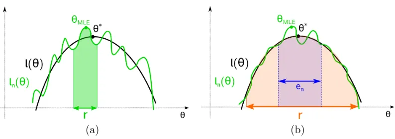
Figure 1: (a) A poorly behaved sample likelihood, for which there are many local optima at varying distances from the MLE. It would require an initialization extremely close to the MLE in order to ensure that the Baum-Welch algorithm would not be trapped at a sub-optimal fixed point. (b) A well-behaved sample likelihood, for which all local optima lie within anen-ball of the MLE, as well as the true parameterθ∗. In this case, the Baum-Welch
algorithm, when initialized within a ball of large radius r, will converge to the ball of much smaller radius en. The goal of this paper is to give sufficient conditions for when the sample
likelihood exhibits this favorable structure.
sufficiently close to the MLE, then it will converge to it. However, the classical analysis does not quantify the size of this neighborhood, and as a critical consequence, itdoes not rule out the pathological type of behavior illustrated in panel (a) of Figure 1. Here the sample likelihood has multiple optima, both a global optimum corresponding to the MLE as well as many local optima far away from the MLE that are also fixed points of the Baum-Welch algorithm. In such a setting, the Baum-Welch algorithm will only converge to the MLE if it is initialized in an extremely small neighborhood.
In contrast, the goal of this paper is to give sufficient conditions under which the sample likelihood has the more favorable structure shown in panel (b) of Figure 1. Here, even though the MLE does not have a large basin of attraction, the sample likelihood has all of its optima (including the MLE) localized to a small region around the true parameter
θ∗. Our strategy to reveal this structure, as in our past work (Balakrishnan et al., 2014), is to shift perspective: instead of studying convergence of Baum-Welch updates to the MLE, we study their convergence to an n-ball of the true parameterθ∗, and moreover,
instead of focusing exclusively on the sample likelihood, we first study the structure of the population likelihood, corresponding to the idealized limit of infinite data. Our first main result (Theorem 1) provides sufficient conditions under which there is a large ball of radiusr, over which the population version of the Baum-Welch updates converge at a geometric rate toθ∗. Our second main result (Theorem 2) uses empirical process theory to analyze the finite-sample version of the Baum-Welch algorithm, corresponding to what is actually implemented in practice. In this finite sample setting, we guarantee that over the ball of radiusr, the Baum-Welch updates will converge to an n-ball withnr, and most
importantly, this n-ball contains the true parameterθ∗. Typically this ball also contains
but rather to a point that is close to both the MLE and the true parameterθ∗ and whose statistical risk is equivalent to that of the MLE upto logarithmic factors.
These latter two results are abstract, applicable to a broad class of HMMs. We then specialize them to the case of a hidden Markov mixture consisting of two isotropic components, with means separated by a constant distance, and obtain concrete guarantees for this model. It is worth comparing these results to past work in the i.i.d. setting, for which the problem of Gaussian mixture estimation under various separation assumptions has been extensively studied (e.g. (Dasgupta, 1999; Vempala and Wang, 2004; Belkin and Sinha, 2010; Moitra and Valiant, 2010)). The constant distance separation required in our work is much weaker than the separation assumptions imposed in most papers that focus on correctly labeling samples in a mixture model. Our separation condition is related to, but in general incomparable with the non-degeneracy requirements in other work (Hsu et al., 2012; Hsu and Kakade, 2013; Moitra and Valiant, 2010).
Finally, let us discuss the various challenges that arise in studying the dependent data setting of hidden Markov models, and highlight some important differences with the i.i.d. setting (Balakrishnan et al., 2014). In the non-i.i.d. setting, arguments passing from the population-based to sample-based updates are significantly more delicate. First of all, it is not even obvious that the population version of theQ-function—a central object in the Baum-Welch updates— exists. From a technical standpoint, various gradient smoothness conditions are much more difficult to establish, since the gradient of the likelihood no longer decomposes over the samples as in the i.i.d. setting. In particular, each term in the gradient of the likelihood is a function of all observations. Finally, in order to establish the finite-sample behavior of the Baum-Welch algorithm, we can no longer appeal to standard i.i.d. concentration and empirical process techniques. Nor do we pursue the approach of some past work on HMM estimation (e.g. (Hsu et al., 2012)), in which it is assumed that there are multiple independent samples of the HMM.1 Instead, we directly analyze the Baum-Welch algorithm that practioners actually use—namely, one that applies to a single sample of an n-length HMM. In order to make the argument rigorous, we need to make use of more sophisticated techniques for proving concentration for dependent data (Yu, 1994; Nobel and Dembo, 1993).
The remainder of this paper is organized as follows. In Section 2, we introduce basic background on hidden Markov models and the Baum-Welch algorithm. Section 3 is devoted to the statement of our main results in the general setting, whereas Section 4 contains the more concrete consequences for the Gaussian output HMM. The main parts of our proofs are given in Section 5, with the more technical details deferred to the appendices.
2. Background and problem set-up
In this section, we introduce some standard background on hidden Markov models and the Baum-Welch algorithm.
2.1 Standard HMM notation and assumptions
We begin by defining a discrete-time hidden Markov model with hidden states taking values in a discrete space. Letting Z denote the integers, suppose that the observed random
variables{Xi}i∈Z take values inRd, and the latent random variables{Zi}i∈Z take values in
the discrete space [s] : ={1, . . . , s}. The Markov structure is imposed on the sequence of latent variables. In particular, if the variable Z1 has some initial distributionπ1, then the joint probability of a particular sequence (z1, . . . , zn) is given by
p(z1, . . . , zn;β) =π1(z1;β) n Y
i=1
p(zi|zi−1;β), (1)
where the vectorβis a particular parameterization of the initial distribution and Markov chain transition probabilities. We restrict our attention to the homogeneous case, meaning that the transition probabilities for step (t−1)→tare independent of the indext. Consequently, if we define the transition matrixA∈Rs×s with entries
A(j, k;β) : =p(z2 =k|z1=j;β),
then the marginal distribution πi ofZi can be described by the matrix vector equation
πTi =π1TAi−1,
where πi andπ1 denote vectors belonging to the s-dimensional probability simplex.
We assume throughout that the Markov chain is aperiodic and recurrent, whence it has a unique stationary distribution π, defined by the eigenvector equation πT =πTA. To be clear, bothπ and the matrixA depend onβ, but we omit this dependence so as to simplify notation. We assume throughout that the Markov chain begins in its stationary state, so thatπ1=π, and moreover, that it is reversible, meaning that
π(j)A(j, k) =π(k)A(k, j) (2)
for all pairs j, k∈[s].
A key quantity in our analysis is the mixing rate of the Markov chain. In particular, we assume the existence ofmixing constant mix∈(0,1] such that
mix≤
p(zi|zi−1;β)
π(zi)
≤−mix1 (3)
for all (zi, zi−1) ∈ [s]×[s]. This condition implies that the dependence on the initial
distribution decays geometrically. More precisely, some simple algebra shows that
sup
π1
π1TAt−πT1
TV≤c0ρ
t
p(zi|zi-1, )
p(x|z, )
X
i-1X
iX
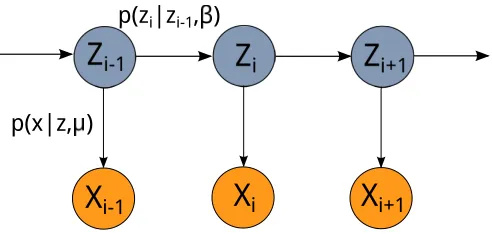
i+1Figure 2: The hidden Markov model as a graphical model. The blue circles indicate observed variablesZi, whereas the orange circles indicate latent variablesXi.
Associated with each latent variable Zi is an observationXi∈Rd. We use p(xi|zi;µ) to
denote the density ofXi given that Zi =zi, an object that we assume to be parameterized
by a vectorµ. Introducing the shorthand xn
1 = (x1, . . . , xn) and z1n= (z1, . . . , zn), the joint
probability of the sequence (xn1, z1n) (also known as the complete likelihood) can be written in the form
p(z1n, xn1;θ) =π1(z1)
n Y
i=2
p(zi |zi−1;β)
n Y
i=1
p(xi|zi;µ), (5)
where the pair θ : = (β, µ) parameterizes the transition and observation functions. The likelihood then reads
p(xn1;θ) =X
zn
1
p(z1n, xn1;θ).
For our convenience in subsequent analysis, we also define a form of complete likelihood including an additional hidden variable z0 which is not associated to any observationx0
p(z0n, xn1;θ) =π0(z0)
n Y
i=1
p(zi |zi−1;β)
n Y
i=1
p(xi|zi;µ), (6)
where π0 = π. Note that it preserves the usual relationship Pzn
0 p(z
n
0, xn1;θ) = p(xn1;θ) between the ordinary and complete likelihoods in EM problems.
A simple example: A special case helps to illustrate these definitions. In particular, suppose that we have a Markov chain withs= 2 states. Consider a matrix of transition probabilities A∈R2×2 of the form
A= 1
eβ+e−β
eβ e−β e−β eβ
=
ζ 1−ζ
1−ζ ζ
, (7)
where ζ : = eβ+eβe−β. By construction, this Markov chain is recurrent and aperiodic
eigenvalues of the transition matrix, we find that the mixing condition (4) holds with
ρmix : =|2ζ−1|=|tanh(β)|.
Suppose moreover that the observed variables in Rdare conditionally Gaussian, say with
p(xt|zt;µ) =
( 1
(2πσ2)d/2 exp
− 1
2σ2kx−µk22 ifzt= 1
1
(2πσ2)d/2 exp
− 1
2σ2kx+µk22 ifzt= 2.
(8)
With this choice, the marginal distribution of each Xt is a two-state Gaussian mixture with
mean vectorsµand −µ, and covariance matricesσ2Id. We provide specific consequences of
our general theory for this special case in the sequel.
2.2 Baum-Welch updates for HMMs
We now describe the Baum-Welch updates for a general discrete-state hidden Markov model. As a special case of the EM algorithm, the Baum-Welch algorithm is guaranteed to ascend on the likelihood function of the hidden Markov model. It does so indirectly, by first computing a lower bound on the likelihood (E-step) and then maximizing this lower bound (M-step).
For a given integer n≥1, suppose that we observe a sequence xn1 = (x1, . . . , xn) drawn
from the marginal distribution overX1ndefined by the model (5). The rescaled log likelihood of the sample path xn1 is given by
`n(θ) =
1
nlog X
zn
0
p(zn0, xn1;θ)
The EM likelihood is based on lower bounding the likelihood via Jensen’s inequality. For any choice of parameter θ0 and positive integers i ≤ j and a < b, let EZj
i|xba,θ0 denote
the expectation under the conditional distribution p(Zij |xba;θ0). With this notation, the concavity of the logarithm and Jensen’s inequality imply that for any choice ofθ0, we have the lower bound
`n(θ) =
1
nlog
EZn
0|xn1,θ0
p(Z0n, xn1;θ)
p(Zn
0 |xn1;θ0)
≥ 1
nEZn0|xn1,θ0
logp(Z0n, xn1;θ)
| {z }
Qn(θ|θ0)
+1
nEZn0|xn1,θ0
−logp(Z0n|xn1;θ0)]
| {z }
Hn(θ0)
.
For a given choice of θ0, the E-step corresponds to the computation of the function
θ7→Qn(θ |θ0). TheM-step is defined by the EM operatorMn:Ωe 7→Ωe
Mn(θ0) = arg max
θ∈Ωe
Qn(θ |θ0), (9)
whereΩ is the set of feasible parameter vectors. Overall, given an initial vectore θ0 = (β0, µ0),
This description can be made more concrete for an HMM, in which case the Q-function takes the form
Qn(θ|θ0) =
1
nEZ0|xn1,θ0
logπ0(Z0;β)
+ 1
n n X
i=1
EZi−1,Zi|xn1,θ0
logp(Zi |Zi−1;β)
+ 1
n n X
i=1
EZi|xn1,θ0
logp(xi |Zi;µ)
, (10)
where the dependence of π0 onβ comes from the assumption thatπ0 =π. Note that the
Q-function can be decomposed as the sum of a term which is solely dependent onµ, and another one which only depends on β—that is
Qn(θ|θ0) =Q1,n(µ|θ0) +Q2,n(β|θ0) (11)
where Q1,n(µ|θ0) = n1Pni=1EZi|xn1,θ0
logp(xi |Zi, µ)
, and Q2,n(β|θ0) collects the
remain-ing terms. In order to compute the expectations definremain-ing this function (E-step), we need to determine the marginal distributions over the singletons Zi and pairs (Zi, Zi+1) under
the joint distribution p(Z0n |xn1;θ0). These marginals can be obtained efficiently using a recursive message-passing algorithm, known either as the forward-backward or sum-product algorithm (Kschischang et al., 2001; Wainwright and Jordan, 2008).
In the M-step, the decomposition (11) suggests that the maximization over the two components (β, µ) can also be decoupled. Accordingly, with a slight abuse of notation, we often write
Mnµ(θ0) = arg max
µ∈Ωµ
Q1,n(µ|θ0), and Mnβ(θ0) = arg max
β∈Ωβ
Q2,n(β|θ0)
for these two decoupled maximization steps, where Ωβ and Ωµ denote the feasible set of
transition and observation parameters respectively and Ω : = Ωe β ×Ωµ. In the following,
unless otherwise stated, Ωµ=Rd, so that the maximization over the observation parameters
is unconstrained.
3. Main results
We now turn to the statement of our main results, along with a discussion of some of their consequences. The first step is to establish the existence of an appropriate population analog of the Q-function. Although the existence of such an object is a straightforward consequence of the law of large numbers in the case of i.i.d. data, it requires some technical effort to establish existence for the case of dependent data; in particular, we do so using a
3.1 Existence of population Q-function
In the analysis of Balakrishnan et al. (2014), the central object is the notion of a population
Q-function—namely, the function that underlies the EM algorithm in the idealized limit of infinite data. In their setting of i.i.d. data, the standard law of large numbers ensures that as the sample sizenincreases, the sample-based Q-function approaches its expectation, namely the function
Q(θ|θ0) =EQn(θ|θ0)
= EEZ1|X1,θ0
logp(X1, Z1;θ)
.
Here we use the shorthandE for the expectation over all samplesX that are drawn from
the joint distribution (in this case E:=EXn
1|θ∗).
When the samples are dependent, the quantity EQn(θ|θ0)
is no longer independent of
n, and so an additional step is required. A reasonable candidate for a general definition of the populationQ-function is given by
Q(θ|θ0) : = lim
n→+∞[EQn(θ|θ
0)]. (12)
Although it is clear that this definition is sensible in the i.i.d. case, it is necessary for dependent sampling schemes to prove that the limit given in definition (12) actually exists.
In this paper, we do so by considering a suitably truncated version of the sample-based
Q-function. Similar arguments have been used in past work (e.g., (Capp´e et al., 2004; van Handel, 2008)) to establish consistency of the MLE; here our focus is instead on the behavior of the Baum-Welch algorithm. Let us consider a sequence {(Xi, Zi)}ni=1+k−k, assumed to be
drawn from the stationary distribution of the overall chain. Recall that EZj
i|xba,θ denotes
expectations taken over the distributionp(Zij |xba, θ). Then, for a positive integerk to be chosen, we define
Qkn(θ|θ0) = 1
n h
EZ0|xk−k,θ0logp(Z1;β) +
n X
i=1
EZi
i−1|x
i+k
i−k,θ0logp(Zi
|Zi−1;β)
+
n X
i=1
EZi|xi+k
i−k,θ
0logp(xi |Zi;µ) i
. (13)
In an analogous fashion to the decomposition in equation (10), we can decomposeQkn in the form
Qkn(θ|θ0) =Qk1,n(µ|θ0) +Qk2,n(β |θ0).
We associate with this triplet of Q-functions the corresponding EM operators Mnk(θ0),
Mnµ,k(θ0) and Mnβ,k(θ0) as in Equation (9). Note that as opposed to the functionQn from
equation (10), the definition ofQkn involves variablesZi, Zi−1 that are not conditioned on the full observation sequence xn
1, but instead only on a 2k window centered around the indexi. By construction, we are guaranteed that the k-truncated population function and its decomposed analogs given by
Qk(θ|θ0) := lim
n→∞EQ
k
n(θ|θ0) =EQk1,n(µ|θ0) + limn→∞EQk2,n(β|θ0)
are well-defined. In particular, due to stationarity of the random sequences{p(zi|Xi−ki+k)}ni=1 and {p(zi−i 1 |Xi−ki+k)}n
i=1, the expectation over {(Xi, Zi)}ni=1+k−k is independent of the sample
sizen. Notice that the Baum-Welch algorithm in practice essentially corresponds to using
k=n.
Our first result uses the existence of this truncated population object in order to show that the standard populationQ-function from equation (12) is indeed well-defined. In doing so, we make use of the sup-norm
kQ1−Q2k∞: = sup
θ,θ0∈
e
Ω
Q1(θ|θ 0)−Q
2(θ|θ0)
. (15)
We require in the following that the observation densities satisfy the following boundedness condition
sup
θ∈Ωe
E h
max
zi∈[s]
logp(Xi |zi, θ) i
<∞. (16)
Proposition 1 Under the previously stated assumptions, the population function Q defined in equation (12)exists.
The proof of this claim is given in Appendix A. It hinges on the following auxiliary claim, which bounds the difference between EQnand thek-truncatedQ-function as
kEQn−Qkk∞≤ c s4
9mixπmin2 1−mixπmin k
+c(πmin, s, mix)
n , (17)
whereπmin:= minβ∈Ωβ,j∈[s]π(j|β) is the minimum probability in the stationary distribution, mix is the mixing constant from equation (3), and c(·) is a constant dependent only on the inherent model parameters. The dependencies on mix and πmin are not optimized here. Since this bound holds for all n, it shows that the population function Q can be uniformly approximated byQk, with the approximation error decreasing geometrically as the truncation level kgrows. This fact plays an important role in the analysis to follow.
3.2 Analysis of updates based on Qk
Our ultimate goal is to establish a bound on the difference between the sample-based Baum-Welch estimate andθ∗, in particular showing contraction of the Baum-Welch update towards the true parameter. Our strategy for doing so involves first analyzing the Baum-Welch iterates at the population level, which is the focus of this section.
The quantity Q is significant for the EM updates because the parameter θ∗ satisfies the self-consistency property θ∗ = arg maxθQ(θ|θ∗). In the i.i.d. setting, the functionQ
the assumption of strong concavity of Qk imply an upper bound on the distance of the maximizers of Qk and Q.
With this setup, we consider an idealized population-level algorithm that, based on some initializationθe0∈Ω =B2 r;µ∗
×Ωβ, generates the sequence of iterates
e
θt+1 =Mk(θet) := arg max
θ∈Ωe
Qk(θ|θet). (18)
where Ω = Ωe β×Ωµ is a larger set than Ω, especially Ωµ=Rd. SinceQk is an approximate
version ofQ, the update operator Mk should be understood as an approximation to the idealized population EM operator M where the maximum is taken with respect toQ. As part (a) of the following theorem shows, the approximation error is well-controlled under suitable conditions. We analyze the convergence of the sequence {θet}∞t=0 in terms of the
norm k · k? : Ωµ×Ωβ →R+ given by
kθ−θ∗k? =k(µ, β)−(µ∗, β∗)k?: =kµ−µ∗k2+kβ−β∗k2. (19) Contraction in this norm implies that both parameters µ, β converge linearly to the true parameter.
Conditions on Qk: Let us now introduce the conditions on the truncated functionQk
that underlie our analysis. For this purpose, we concentrate on a potentially smaller set
Ω : =B2(r;µ∗)×Ωβ
with radiusr >0, where Ωβ is the set of allowable HMM transition parameters. The goal is
to find the largest Ω⊂Ω, in which said conditions are fulfilled. This set Ω is then equivalente
to the basin of attraction, i.e. the set in which we can initialize the algorithm and obtain linear convergence to a good optimum.
First, let us say that the functionQk(· |θ0) is (λµ, λβ)-strongly concave in Ω if for all θ0 ∈Ω we have
Qk1(µ1 |θ0)−Qk1(µ2 |θ0)− h∇µQk1(µ2 |θ0), µ1−µ2i ≤ −
λµ
2 kµ1−µ2k 2
2 (20a) and Qk2(β1|θ0)−Qk2(β2 |θ0)− h∇βQk2(β2 |θ0), β1−β2i ≤ −
λβ
2 kβ1−β2k 2
2 (20b) for all (µ1, β1),(µ2, β2)∈Ω.
Second, we impose first-order stability conditions on the gradients of each component of
Qk:
• For eachµ∈Ωµ, θ0 ∈Ω, we have
k∇µQk1(µ|µ0, β0)− ∇µQk1(µ|µ∗, β0)k2≤Lµ,1kµ0−µ∗k2 (21a) k∇µQk1(µ|µ0, β0)− ∇µQk1(µ|µ0, β∗)k2≤Lµ,2kβ0−β∗k2, (21b) We refer to this condition as Lµ-FOS for short.
• Secondly, for allβ ∈Ωβ, θ0 ∈Ω, we require that
We refer to this condition as Lβ-FOS for short. The experienced reader may find that
the (Lµ, Lβ)-FOS conditions look intriguingly similar to the Lipschitz gradient conditions
often encountered when proving geometric convergence for gradient descent methods. On a high level, smoothness requires function values of one function to be close for any pair of arguments that are close. Although our conditions seem to invoke Lipschitz gradients as well, it is actually of a completely different nature. The important difference arises from the existence of two parameters, as we now clarify.
As opposed to gradient descent, the EM updates optimize over the first parameter θ
of a functionQk(· |θ0) defined by the second parameter θ0 at every time step. If we could access Qk(· |θ∗), EM would converge in one step to the true optimum. Therefore, if we can guarantee thatQk(· |θ0) andQk(· |θ∗) are close in some sense, there should be good reasons to hope that under some more regularity assumptions the maximizers are close as well, i.e. that Mk(θ0) is close toθ∗.
The (Lµ, Lβ)-FOS conditions are precisely encouraging closeness of these two functions in
a first-order sense. In particular, we require the gradients (with respect to the first argument
θ) to be Lipschitz in the second argument θ0. Typical smoothness however is a property with respect to a fixed function (i.e. a fixedθ0 in our case) and thus requires gradients to be Lipschitz in the first argument. Loosely speaking it upper bounds the curvature of said function, and thus is more like a second-order condition by nature. This distinction also explains why (Lµ, Lβ)-FOS conditions require to be uniformly satisfied only over the first
argument, while one of the second arguments can be fixed at µ∗ or β∗ respectively. Finally, as we show in Section 4, these conditions hold for concrete models.
Convergence guarantee for Qk-updates: We are now equipped to state our main convergence guarantee for the updates. It involves the quantities
L: = max{Lµ1, Lµ2}+ max{Lβ1, Lβ2}, λ: = min{λµ, λβ} and κ: =
L
λ, (23)
with κ generally required to be smaller than one, as well as the additive normk · k? from equation (19).
Part (a) of the theorem controls theapproximation error induced by using thek-truncated functionQk as opposed to the exact population function Q, whereas part (b) guarantees a geometric rate of convergence in terms ofκ defined above in equation (23).
Theorem 1 (a) Approximation guarantee: Under the mixing condition (4), density bound-edness condition (16), and (λµ, λβ)-strong concavity condition (20), there is a universal
constant c0 such that
kMk(θ)−M(θ)k2? ≤ Cs 4
λ 9 mixπmin2
1−mixπmink
| {z }
=:ϕ2(k)
for all θ∈Ω, (24)
where s is the number of states, and πmin : = min
β∈Ωβ
min
j∈[s]π(j;β).
(b) Convergence guarantee: Suppose in addition that the (Lµ, Lβ)-FOS conditions (21),(22)
holds with parameter κ∈(0,1) as defined in (23) for θ, θ0 ∈Ω =B2 r;µ∗
that the truncation parameter k is sufficiently large to ensure that
ϕ(k)≤ 1−κ
r−κmax
β∈Ωβ
kβ−β∗k2.
Then, given an initializationθe0∈Ω, the iterates {θet}∞t=0 generated by the Mk operator
satisfy the bound
kθet−θ∗k? ≤κtkθe0−θ∗k?+
1
1−κϕ(k). (25)
Note that the subtlety here is that θ∗ is no longer a fixed point of the operator Mk, due to the error induced by thekth-order truncation. Nonetheless, under the mixing condition, as the bounds (24) and (25) show, this approximation error is controlled, and decays exponentially ink. The proof of the recursive bound (25) is based on showing that
kMk(θ)−Mk(θ∗)k? ≤κkθ−θ∗k? (26)
for anyθ∈Ω. Inequality (26) is equivalent to stating that the operator Mk is contractive, i.e. that applyingMk to the pair θ and θ∗ always decreases the distance.
Finally, when Theorem 1 is applied to a concrete model, the task is to find a big r and Ωβ such that the conditions in the theorem are satisfied, and we do so for the Gaussian
output HMM in Section 4.
3.3 Sample-based results
We now turn to a result that applies to the sample-based form of the Baum-Welch algorithm— that is, corresponding to the updates that are actually applied in practice. For a tolerance parameterδ ∈(0,1), we letϕn(δ, k) be the smallest positive scalar such that
P h
sup
θ∈Ω
kMn(θ)−Mnk(θ)k? ≥ϕn(δ, k) i
≤δ. (27a)
This quantity bounds the approximation error induced by the k-truncation, and is the sample-based analogue of the quantity ϕ(k) appearing in Theorem 1(a). For eachδ∈(0,1), we let µn(δ, k) and βn(δ, k) denote the smallest positive scalars such that
Psup
θ∈Ω
kMnµ,k(θ)−Mµ,k(θ)k2≥µn(δ, k)i≤δ, and (27b)
Psup
θ∈Ω
kMnβ,k(θ)−Mβ,k(θ)k2≥βn(δ, k) i
≤δ,
where Mnµ,k(·) and Mnβ,k(·) correspond to the truncated versions of Mnµ(·) and Mnβ(·).
Furthermore we definen(δ, k) : =µn(δ, k) +βn(δ, k). For a given truncation levelk, these
values give an upper bound on the difference between the population and sample-based
Theorem 2 (Sample Baum-Welch) Suppose that the truncated population EM operator Mk satisfies the local contraction bound (26) with parameterκ ∈(0,1) in Ω. For a given sample size n, suppose that (k, n) are sufficiently large to ensure that
ϕn(δ, k) +ϕ(k) +µn δ, k
≤(1−κ)r−κmax
β∈Ωβ
kβ−β∗k2. (28a)
Then given any initialization θb0 ∈ Ω, with probability at least 1−2δ, the Baum-Welch
sequence {θbt}∞t=0 satisfies the bound
kbθt−θ∗k? ≤ κtkθb0−θ∗k?
| {z }
Geometric decay + 1
1−κ n
ϕn δ, k
+ϕ(k) +n δ, k o
| {z }
Residual error en
. (28b)
The bound (28b) shows that the distance between θbt andθ∗ is bounded by two terms:
the first decays geometrically as tincreases, and the second term corresponds to a residual error term that remains independent oft. Thus, by choosing the iteration numberT larger than log(2logr/κ ), we can ensure that the first term is at most. The residual error term can be controlled by requiring that the sample size nis sufficiently large, and then choosing the truncation levelkappropriately. We provide a concrete illustration of this procedure in the following section, where we analyze the case of Gaussian output HMMs. In particular, we can see that the residual error is of the same order as for the MLE and that the required initialization radius is optimal up to constants. Let us emphasize here thatk as well as the truncated operators are purely theoretical objects which were introduced for the analysis.
4. Concrete results for the Gaussian output HMM
We now return to the concrete example of a Gaussian output HMM, as first introduced in Section 2.1, and specialize our general theory to it. Before doing so, let us make some preliminary comments about our notation and assumptions. Recall that our Gaussian output HMM is based on s= 2 hidden states, using the transition matrix from equation (7), and the Gaussian output densities from equation (8). For convenience of analysis, we let the hidden variablesZi take values in{−1,1}. In addition, we require that the mixing coefficient ρmix = 1−mix is bounded away from 1 in order to ensure that the mixing condition (3) is fulfilled. We denote the upper bound for ρmix as b <1 so that ρmix ≤b and mix ≥1−b. The feasible set of the probability parameterζ and its log odds analog β = 12log 1−ζζ are then given by
Ωζ =
ζ ∈R| 1
−b
2 ≤ζ ≤ 1 +b
2
, and Ωβ =
n
β ∈R | |β|< 1
2log 1 +b
1−b
| {z }
βB
4.1 Explicit form of Baum-Welch updates
We begin by deriving an explicit form of the Baum-Welch updates for this model. Using this notation, the Baum-Welch updates take the form
b
µt+1 = 1
n n X
i=1
(2p(Zi = 1|xn1;θbt)−1)xi, (30a)
b
ζt+1 = ΠΩζ
1
n n X
i=1
X
Zi
p(Zi =Zi+1|xn1;θbt)
, and (30b)
b
βt+1 = 1 2log
b ζt+1
1−ζbt+1
, (30c)
where ΠΩζ denotes the Euclidean projection onto the set Ωζ. Note that the maximization
steps are carried out on the decomposed Q-functions Q1,n(· |θt), Q2,n(· |θt). In addition,
since we are dealing with a one-dimensional quantity β, the projection of the unconstrained maximizer onto the interval Ωζ is equivalent to the constrained maximizer over the feasible
set Ωζ. This step is in general not valid for higher dimensional transition parameters.
4.2 Population and sample guarantees
We now use the results from Section 3 to show that the population and sample-based version of the Baum-Welch updates are linearly convergent in a ball around θ∗ of fixed radius. In establishing the population-level guarantee, the key conditions which need to be fulfilled—and the one that are the most technically challenging to establish— are the (Lµ, Lβ)-FOS conditions (21), (22). In particular, we want to show that these conditions
hold with Lipschitz constantsLµ, Lβ that decrease exponentially with the separation of the
mixtures. As a consequence, we obtain that for large enough separation Lλ <1, i.e. the EM operator is contractive towards the true parameter.
In order to ease notation, our explicit tracking of parameter dependence is limited to the standard deviationσand Euclidean normkµ∗k2, which together determine the signal-to-noise ratioη2: = kµ∗k22
σ2 of the mixture model. Throughout this section, we therefore usec0, c1 to denote universal constants andC0, C1 for quantities that do not depend on (kµ∗k2, σ), but may depend on other parameters such as πmin,ρmix,b, and so on.
We begin by stating a result for the sequence {θet}∞t=0 obtained by repeatedly applying
the k-truncated population-level Baum-Welch update operator Mk. Our first corollary establishes that this sequence is linearly convergent, with a convergence rateκ=κ(η) that is given by
κ(η) : = C1η
2(η2+ 1) e−c2η2
1−b2 . (31)
Corollary 1 (Population Baum-Welch) Consider a two-state Gaussian output HMM that is mixing (i.e. satisfies equation (3)), and with its SNR lower bounded as η2 ≥C for a sufficiently large constant C. Given the radius r = kµ∗k2
parameterkis sufficiently large to ensure that ϕ(k)≤(1−κ)r−κmaxβ∈Ωβkβ−β ∗k
2. Then for any initialization θe0 = (eµ0,βe0)∈B2 r;µ∗
×Ωβ, the sequence{θet}∞t=0 generated by Mk
satisfies the bound
kθet−θ∗k? ≤κtkθe0−θ∗k?+
1
1−κϕ(k) (32)
for all iterations t= 1,2, . . ..
From definition (31) it follows that as long as the signal-to-noise ratio η is larger than a universal constant, the convergence rateκ(η)<1. The bound (32) then ensures a type of contraction and the pre-conditionϕ(k)≤(1−κ)r−κmaxβ∈Ωβkβ−β
∗k
2 can be satisfied by choosing the truncation parameterk large enough. If we use a finite truncation parameter
k, then the contraction occurs up to the error floor given byϕ(k), which reflects the bias introduced by truncating the likelihood to a window of sizek. At the population level (in which the effective sample size is infinite), we could take the limit k→ ∞ so as to eliminate this bias. However, this is no longer possible in the finite sample setting, in which we must necessarily have kn. While largekgive a better truncation approximation, it allows for fewer samples which are “sufficiently independent” from each other within the sequence. We can see in the proof of Corollary 2 that k%logn is a good choice to obtain an adequate trade-off.
Corollary 2 (Sample Baum-Welch iterates) For a given toleranceδ ∈(0,1), suppose that the sample size is lower bounded as n≥ C1
kµ∗k2 2σ2
(η2+ 1)3dlog8(dδ). Then under the conditions of Corollary 1 and η2≥Clog 1
1−b2, with probability at least 1−δ, we have
kθet−θ∗k? ≤κtkθb0−θ∗k?+ C σ
kµ∗k2 2
σ2 + 1
3/2q
dlog8(n/δ)
n
1−κ . (33)
Remarks: As a consequence of the bound (33), if we are given a sample sizen%dlog8d, then taking T ≈logniterations is guaranteed to return an estimate (bµT,βbT) with error of
the order
q
dlog8(n)
n .
In order to interpret this guarantee, note that in the case of symmetric Gaussian output HMMs as in Section 4, standard techniques can be used to show that the minimax rate of
estimatingµ∗ in Euclidean norm scales as
q d
n. If we could compute the MLE in polynomial
time, then its error would also exhibit this scaling. The significance of Corollary 2 is that it shows that the Baum-Welch update achieves this minimax risk of estimation up to logarithmic factors.
4.3 Simulations
In this section, we provide the results of simulations that confirm the accuracy of our theoretical predictions for two-state Gaussian output HMMs. In all cases, we update the estimates for the mean vectorµbt+1 and transition probability ˆζt+1according to equation (30); for convenience, we updateζ as opposed to β. The true parameters are denoted byµ∗ and
ζ∗.
5 10 15
−8 −6 −4 −2
Iteration numbert
L
og
er
ror
log10kµˆti−µˆ1k2
log10kµˆti−µ∗k2
Figure 3: Plot of the convergence of the optimization error logkµbti−µb1k2, plotted in blue, and the statistical error logkbµti −µ∗k2, plotted in red, for 5 different initializations. The parameter settings wered= 10,n= 1000, ρmix= 0.6 and SNR kµ
∗k
2
σ = 1.5. See the main
text for further details.
In all simulations, we fix the mixing parameter to ρmix = 0.6, generate initial vectors
b
µ0 randomly in a ball of radiusr : = kµ∗k2
4 around the true parameter µ
∗, and set b ζ0 = 12. Finally, the estimation error of the mean vector µ is computed as log10kµˆ−µ∗k2. Since the transition parameter estimation errors behave similarly to the observation parameter in simulations, we omit the corresponding figures here.
Figure 3 depicts the convergence behavior of the Baum-Welch updates, as assessed in terms of both the optimization and the statistical error. Here we run the Baum-Welch algorithm for a fixed sample sequenceXn
1 drawn from a model with SNRη2 = 1.5 andζ = 0.2, using different random initializations in the ball aroundµ∗ with radius kµ∗k2
4 . We denote the final estimate of thei−th trial by µbi. The curves in blue depict theoptimization error—that
is, the differences between the Baum-Welch iterates bµti using the i-th initialization, and µb1. On the other hand, the red lines represent the statistical error—that is, the distance of the iterates from the true parameterµ∗.
For both family of curves, we observe linear convergence in the first few iterations until an error floor is reached. The convergence of the statistical error aligns with the theoretical prediction in upper bound (33) of Corollary 2. The (minimax-optimal) error floor in the curve corresponds to the residual error and theen–region in Figure 1. In addition, the blue
optimization error curves show that for different initializations, the Baum-Welch algorithm converges todifferent stationary points µbi; however, all of these points have roughly the same
in our analysis—that is, focusing on the true parameter as opposed to the MLE. Given the presence of all these local optima in a small neighborhood ofµ∗, the basin of attraction of the MLE must necessarily be much smaller than the initialization radius guaranteed by our theory.
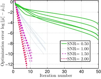
Figure 4 shows how the convergence rate of the Baum-Welch algorithm depends on the underlying SNR parameter η2; this behavior confirms the predictions given in Corollary 2. Lines of the same color represent different random draws of parameters given a fix SNR. Clearly, the convergence is linear for high SNR, and the rate decreases with decreasing SNR.
0 10 20 30 40 50
−12 −10 −8 −6 −4 −2 0
Iteration number
O
p
ti
m
iz
at
ion
er
ror
log
k
ˆ
µ
t−i
ˆ
µ
i
k2
SNR= 0.50 SNR= 1.00 SNR= 1.50 SNR= 2.00
Figure 4: Plot of convergence behavior for different SNR, where for each curve, different parameters were chosen. The parameter settings are d= 10,n= 1000 andρmix = 0.6.
5. Proofs
In this section, we collect the proofs of our main results. In all cases, we provide the main bodies of the proofs here, deferring the more technical details to the appendices.
5.1 Proof of Theorem 1
Throughout this proof, we make use of the shorthand ρemix= 1−mixπmin. Also we denote
the separate components of the population EM operators by M(θ) =: (Mµ(θ), Mβ(θ))T and their truncated equivalents by Mk(θ) =: (Mµ,k(θ), Mβ,k(θ))T. We begin by proving the bound given in part (a). SinceQ= limn→∞E[Qn], we have
kQ−Qkk∞=k lim
n→∞E[Qn]−Q
kk
∞ ≤
Cs4 9
mixπ2min
e ρkmix,
where we have exchanged the supremum and the limit before applying the bound (17). The same holds for the separate functionsQ1, Q2.
Using this bound and the fact that forQ1 we have Q1(Mµ(θ)|θ)≥Q1(Mµ,k(θ)|θ), we find that
Q1(Mµ(θ)|θ)≥Qk1(Mµ,k(θ)|θ)−
Cs4 9mixπmin2 ρe
k
Since Mµ,k(θ) is optimal, the first-order conditions for optimality imply that
hQk1(Mµ,k(θ)|θ), θ−Mµ,k(θ)i ≤0 for allθ∈Ω. Combining this fact with strong concavity ofQk(·|θ) for all θ, we obtain
Cs4
9 mixπmin2
e
ρkmix≥Qk1(Mµ,k(θ)|θ)−Q1(Mµ(θ)|θ)
≥Qk1(Mµ,k(θ)|θ)−Qk1(Mµ(θ)|θ)− Cs 4
9 mixπmin2
e ρkmix
≥ λµ 2 kM
µ(θ)−Mµ,k(θ)k2
2−
Cs4 9mixπmin2 ρe
k
mix and therefore kMµ(θ)−Mµ,k(θ)k2
2 ≤ 4 Cs
4
λ9
mixπmin2 e
ρk
mix. In particular, setting θ = θ∗ and identifiability, i.e. Mµ(θ∗) =θ∗, yields
kMµ,k(θ∗)−θ∗k22≤4 Cs 4
λµ9mixπmin2 e ρkmix,
and the equivalent bound can be obtained for Mβ,k(·) which yields the claim.
We now turn to the proof of part (b). Let us suppose that the recursive bound (26) holds, and use it to complete the proof of this claim. We first show that if µet ∈B2(r;µ∗), then we must have µet+1 ∈
B2(r;µ∗) as well. Indeed, ifµe
t∈
B2(r;µ∗), then we have by triangle inequality and contraction in (26)
kMµ,k(θet)−µ∗k2≤ kMµ,k(θet)−Mµ,k(θ∗)k2+kMµ,k(θ∗)−µ∗k2
≤κ[kµet−µ∗k2+kβet−β∗k2] +ϕ(k)
≤κ(r+ max
β∈Ωβ
kβ−β∗k2) +ϕ(k)≤r,
where the final step uses the assumed bound on ϕ. For the joint parameter update we in turn have
kMk(θet)−θ∗k? ≤ kMk(θet)−Mk(θ∗)k?+kMk(θ∗)−θ∗k?
≤κkθet−θ∗k?+ϕ(k). (34)
By repeatedly applying inequality (34) and summing the geometric series, the claimed bound (25) follows.
It remains to prove the bound (26). Since the vector Mk(θ∗) maximizes the function
θ7→Qk1(θ|θ∗), we have the first-order optimality condition
h∇Qk1(Mµ,k(θ∗)|θ∗), Mµ,k(θ)−Mµ,k(θ∗)i ≤0, valid for any θ.
Similarly, we haveh∇Qk1(Mµ,k(θ)|θ), Mµ,k(θ∗)−Mµ,k(θ)i ≤0, and adding together these two inequalities yields
On the other hand, by the λ-strong concavity condition, we have
λµkMµ,k(θ)−Mµ,k(θ∗)k22 ≤ h∇Qk1(Mµ,k(θ)|θ
∗
)− ∇Qk1(Mµ,k(θ∗)|θ∗), Mµ,k(θ∗)−Mµ,k(θ)i Combining these two inequalities with the (Lµ, Lβ)-FOS condition yields
λµkMµ,k(θ)−Mµ,k(θ∗)k22 ≤ h∇Qk1(Mµ,k(θ)|θ
∗
)− ∇Qk1(Mµ,k(θ)|θ), Mµ,k(θ∗)−Mµ,k(θ)i ≤
Lµ1kµ−µ
∗k
2+Lµ2kβ−β
∗k
2
kMµ,k(θ)−Mµ,k(θ∗)k2, and similarly we obtainλβkMβ,k(θ)−Mβ,k(θ∗)k2 ≤
Lβ1kµ−µ
∗k
2+Lβ2kβ−β
∗k
2
. Adding both inequalities yields the claim (26).
5.2 Proof of Theorem 2
By the triangle inequality and inequality (34), we have with probability at least 1−2δ that for any iteration
kθbt+1−θ∗k? ≤ kMn(θbt)−Mnk(θbt)k?+kMnk(θbt)−Mk(θbt)k?+kMk(θbt)−θ∗k?
≤ϕn(δ, k) +n(δ, k) +κkθbt−θ∗k?+ϕ(k).
In order to see that the iterates do not leave B2 r;µ∗
, observe that
kµbt+1−µ∗k2≤ kMnµ(θbt)−Mnµ,k(θbt)k2+kMnµ,k(θbt)−Mµ,k(θbt)k2+kMµ,k(θbt)−µ∗k2
≤ϕn(δ, k) +nµ(δ, k) +κ(kµb
t−µ∗k
2+ max
β∈Ωβ
kβ−β∗k2) +ϕ(k). (35)
Consequently, as long askµbt−µ∗k2≤r, we also havekµbt+1−µ∗k2 ≤r whenever
ϕn(δ, k) +ϕ(k) +µn(δ, k)≤(1−κ)r−κβ∈max
Ωβ
kβ−β∗k2. Combining inequality (35) with the equivalent bound for β, we obtain
kθbt−θ∗k?≤κkθbt−1−θ∗k?+ϕn(δ, k) +n(δ, k) +ϕ(k)
Summing the geometric series yields the bound (28b).
5.3 Proof of Corollary 1
The boundedness condition (Assumption (16)) is easy to check since for X∼N(µ∗, σ2), the quantity sup
µ∈B2(r;µ∗)
Emax{kX−µk2,kX+µk2}
is finite for any choice of radius r <∞.
By Theorem 1, the k-truncated population EM iterates satisfy the bound
kθet−θ∗k?≤κtkθe0−θ∗k?+
1
1−κϕ(k), (36)
if the strong concavity (20) and FOS conditions (21), (22) hold with suitable parameters. In the remainder of proof—and the bulk of the technical work— we show that:
• the FOS conditions hold with
Lµ,1 =c (η2+ 1)ϕ2(mix)η2e−cη
2
, and Lµ,2 =c
q
kµ∗k2
2+σ2ϕ2(mix)η2e−cη
2
Lβ,1=c 1−b
1 +bϕ2(mix)η
2e−cη2
and Lβ,2 =c
q
kµ∗k2
2+σ2ϕ2(mix)η2e
−cη2
,
where ϕ2(mix) : =
1
log(1/(1−mix)) +
1
mix
. Substuting these choices into the bound (36) and performing some algebra yields the claim.
5.3.1 Establishing strong concavity
We first show concavity of Qk1(· | θ0) and Qk2(· | θ0) separately. For strong concavity of
Qk1(· |θ0), observe that
Qk1(µ|θ0) =−1 2E
h
p(z0 = 1|X−kk ;θ0)kX0−µk22+ (1−p(z0 = 1|X−kk ;θ0))kX0+µk22+c]
i ,
where cis a quantity independent of µ. By inspection, this function is strongly concave inµ
with parameter λµ= 1.
On the other hand, we have
Qk2(β |θ0) =EXk
−k|θ∗ X
z0,z1
p(z0, z1 |X−kk ;θ0) log
eβz0z1
eβ + e−β
.
This function has second derivative ∂β∂22Qk2(β|θ0) =−4 e
−2β
(e−2β+1)2. As a function of β ∈Ωβ,
this second derivative is maximized atβ = 12log 1+1−bb. Consequently, the functionQk2(· |θ0) is strongly concave with parameter λβ ≥ 23(1−b2).
5.3.2 Separate FOS conditions
We now turn to proving that the FOS conditions in equations (21) and (22) hold. A key ingredient in our proof is the fact that the conditional densityp(z−kk |xk−k;µ, β) belongs to the exponential family with parametersβ ∈R, andγi: = hµ, xσ2ii ∈Rfor i=−k, . . . , kwhich
define the vectorγ = (γ−k, . . . , γk) (see Wainwright and Jordan (2008) for more details on
exponential families.) In particular, we have
p(zk−k|xk−k, µ, β)
| {z }
: =p(zk
−k;γ,β)
= exp
( k X
`=−k
γ`z`+β
k−1
X
`=−k
z`z`+1−Φ(γ, β)
)
, (37)
where the function h absorbs various coupling terms. Note that this exponential family is a specific case of the following exponential family distribution
˜
p(zk−k |xk−k, µ, β)
| {z }
: = ˜p(zk
−k;γ,β)
= exp
( k X
`=−k
γ`z`+
k−1
X
`=−k
β`z`z`+1−Φ(γ, β)
)
The distribution in (37) corresponds to (38) withβ`=β for all` and the so-called partition
function Φ is given by
Φ(γ, β) = logX
z
exp
( k X
`=−k
γ`z`+
k−1
X
`=−k
β`z`z`+1
)
.
The reason to view our distribution as a special case of the more general one in (38) becomes clear when we consider the equivalence of expectations and the derivatives of the cumulant function ∂Φ ∂γ` θ0
=EZk
−k|xk−k,θ0Z` and ∂Φ ∂β0 θ0
=EZk
−k|xk−k,θ0Z0Z1, (39)
where we recall that EZk
−k|x k
−k,θ
0 is the expectation with respect to the distribution ˜p(Z−kk |
xk
−k;µ0, β0) with β` = β0. Note that in the following any value θ0 for ˜p is taken to be on
the manifold on which β` =β0 for someβ0 since this is the manifold the algorithm works
on. Also, as before,E denotes the expectation over the joint distribution of all samples X`
drawn according top(·;θ∗), in this caseXk −k.
Similarly to equations (39), the covariances of the sufficient statistics correspond to the second derivatives of the cumulant function
∂2Φ
∂β`∂β0
θ
= cov(Z0Z1, Z`Z`+1 |X−kk , θ) (40a) ∂2Φ
∂γ`∂γ0
θ
= cov(Z0, Z`|X−kk , θ) (40b) ∂2Φ
∂β`∂γ0
θ
= cov(Z0, Z`Z`+1|X−kk , θ). (40c)
In the following, we adopt the shorthand
cov(Z`, Z`+1|γ0, β0) = cov(Z`, Z`+1|X−kk , θ0)
=EZ`+1
` |X−kk,θ0(Z`
−EZ`+1
` |Xk−k,θ0Z`)(Z`+1
−EZ`+1
` |X−kk,θ0Z`+1)
where the dependence onβ is occasionally omitted so as to simplify notation.
5.3.3 Proof of inequality (21a)
By an application of the mean value theorem, we have
k∇µQk1(µ|µ0, β0)− ∇µQk1(µ|µ∗, β0)k ≤
E k X
`=−k
∂2Φ
∂γ`∂γ0
θ=θe
(γ`0−γ`∗)X0
| {z }
T1
where eθ=θ0+t(θ∗−θ0) for some t∈(0,1). Since second derivatives yield covariances (see
equation (40)), we can write
T1 =
k X
`=−k
EX0E
cov(Z0, Z` |eγ)
so that it suffices to control the expected conditional covariance. By the Cauchy-Schwarz inequality and the fact that cov(X, Y)≤√varX√varY and var(Z0|X)≤1, we obtain the following bound on the expected conditional covariance by using Lemma 4 (see Appendix B)
Ecov(Z0, Z`|γe)|X0
≤pE[var(Z0 |eγ)|X0] p
E[var(Z`|eγ)|X0]
≤pvar(Z0|γe0). (41a)
Furthermore, by Lemma 5 and 6 (see Appendix B), we have
|cov(Z0, Z`|γe)| ≤2ρ `
mix, and
E(var(Z0|eγ0))
1/2X 0X0T
op
≤Ce−cη2. (41b)
From the definition of the operator norm, we have
kEcov(Z0, Z`|eγ)X0X T `
op= sup kuk2=1
kvk2=1
Ecov(Z0, Z`|eγ)hX0, vi hX`, ui
≤ sup
kvk2=1
E|cov(Z0, Z` |eγ)|hX0, vi
2 + sup
kuk2=1
E|cov(Z0, Z` |eγ)|hX`, ui
2 =kEX0X0TE
|cov(Z0, Z` |eγ)|X0
kop
+kEX`X`TE
cov(Z0, Z`|eγ)|X`
kop
(i)
≤2 min{ρ|`|mixkEX0X0Tkop,kEvar(Z0 |eγ0)
1/2X
0X0Tkop}
(ii)
≤ 2 min{(kµ∗k22+σ2)ρ|`|mix, C0e−cη2}, (42) where inequality (i) makes use of inequalities (41a) and (41b), and step (ii) makes use of the second inequality in line (41b).
By inequality (42), we find that
T1 ≤
kµ0−µ∗k2
σ2
k X
`=−k
kEcov(Z0, Z` |eγ)X0X T `
op
≤2kµ
0−µ∗k
2
σ2
k X
`=−k
min{(kµ∗k22+σ2)ρ|`|mix, Ce−cη2}
≤4(η2+ 1) mCe−cη2 + ρ
m
mix 1−ρmix
kµ0−µ∗k2.
where m = log(1cη/ρ2
mix) is the smallest integer such that ρ
m
mix≤ Ce
−cη2
The last inequality follows from the proof of Corollary 1 in the paper Balakrishnan et al. (2014) if η2 > C for some universal constantC. We have thus shown that
k∇µQk1(µ|µ0, β0)− ∇µQk1(µ|µ∗, β0)k ≤Lµ,1kµ0−µ∗k2, where Lµ,1 =c ϕ1(η)ϕ2(mix)η2(η2+ 1)e−cη
2
5.3.4 Proof of inequality (21b)
The same argument via the mean value theorem guarantees that
k ∂
∂βQ k
2(β|µ
0, β0)− ∂ ∂βQ
k
2(β|µ
0, β∗)k ≤ E k X
`=−k
∂2Φ
∂β`∂γ0
θ=eθ
(β0−β∗)X0
2 .
In order to bound this quantity, we again use the equivalence (40) and bound the expected conditional covariance. Furthermore, Lemma 5 and 6 yield
cov(Z0, Z`Z`+1 |eγ)
(i)
≤2ρ`mix and Evar(Z0|γe0)X0X0T
op
(ii)
≤ ce−cη2. (43)
Here inequality (ii) follows by combining inequality (54c) from Lemma 5 with the fact that var(Z0 |eγ0)≤1.
kEX0cov(Z0, Z`Z`+1|eγ)k2 = sup kuk2=1
EhX0, uicov(Z0, Z`Z`+1 |eγ)
≤ sup
kuk2=1
E|hX0, ui|E|cov(Z0, Z`Z`+1|eγ)| |X0
(iii) ≤ sup
kuk2=1
E|hX0, ui|min{ρ
|`|
mix,(var(Z0 |eγ0))
1/2} (iv)
≤ min{ sup
kuk2=1
p
EhX0, ui2ρ
|`|
mix, sup
kuk2=1
p
EhX0, ui2var(Z0 |eγ0))}
(v)
≤ min{ρ|`|mix q
kEX0X0Tkop, q
kEvar(Z0 |eγ0)X0X T
0kop} (vi)
≤ min{ρ|`|mix q
kµ∗k2
2+σ2, Ce
−cη2
}
where step (iii) uses inequality (43); step (iv) follows from the Cauchy-Schwarz inequality; step (v) follows from the definition of the operator norm; and step (vi) uses inequality (43) again.
Putting together the pieces, we find that
E k X
`=−k
∂2Φ
∂β`∂γ0
X0 2
|β0−β∗| ≤
k X
`=−k
kEX0E[cov(Z0, Z`Z`+1 |eγ)|X0]k2|β 0−β∗|
≤4
q
kµ∗k2 2+σ2
c me−cη2 + ρ
m
mix 1−ρmix
|β0−β∗|.
again with m= log(1cη/ρ2
mix), we find that inequality (21b) holds with
Lµ,2 =cϕ2(mix)
p
kµ∗k
2+σ2η2e−cη
2
, as claimed.
5.3.5 Proof of inequality (22a)
By the same argument via the mean value theorem, we find that
∂ ∂βQ
k
2(β|β0, µ0)−
∂ ∂βQ
k
2(β|β0, µ∗)
≤ E k X
`=−k
∂2Φ
∂γ`∂β0
θ=θe
hµ0−µ∗, X`i σ2
Equation (40) guarantees that ∂γ∂2Φ
`∂β0 = cov(Z0Z1, Z` |γ). Therefore, by similar arguments
as in the proof of inequalities (21), we have
T : =
k X
`=−k
Ehµ0−µ∗, X`iE[cov(Z0Z1, Z` |eγ`, β 0
)|X`]
≤
k X
`=−k
E|hµ0−µ∗, X`i|min{ρ
|`|
mix,(var(Z` |eγ`, β 0))1/2}
≤
k X
`=−k
min
ρ|`|mix,pEvar(Z`|eγ`, β 0) p
Ehµ0−µ∗, X`i2
≤
q
kµ∗k2
2+σ2 mce
−cη2
+ 2
k X
`=m+1
ρ`mix.
where we have used inequality (54b) from Lemma 6. Finally, again noting thatm= log(1cη/ρ2
mix)
yields that the FOS condition holds withLβ,2 =c
p
kµ∗k2+σ2ϕ2(mix)η2e−cη
2
, as claimed.
5.3.6 Proof of inequality (22b)
By the same mean value argument, we find that
k ∂
∂βQ k
2(β|β
0
, µ0)− ∂
∂βQ k
2(β|β
∗
, µ0)≤ E
k X
`=−k
∂2Φ
∂β`∂β0
θ=eθ
(β0−β∗)
.
By the exponential family view in equality (40) it suffices to control the expected conditional covariance. Lemma 5 and 6 guarantee that
|cov(Z0Z1, Z`Z`+1|X−kk ,eγ)| ≤ρ |`|
mix, and Evar(Z0Z1 |eγ
1
0,βe)≤c
1 +b
1−b e −cη2
. (44)
Furthermore, the Cauchy-Schwarz inequality combined with the bound (53a) from Lemma 4 yields
Ecov(Z0Z1, Z`Z`+1|eγ)
≤
q
Evar(Z0Z1|γ,e βe)
q
Evar(Z`Z`+1|eγ,βe)
≤
q
Evar(Z0Z1|γe
1 0,βe)
q
Evar(Z`Z`+1|γe
`+1
` ,βe)
≤Evar(Z0Z1 |eγ
1
Combining the bounds (44) and (45) yields k X
`=−k
E ∂
2Φ
∂β`∂β0
(β0−β∗)
≤ k X
`=−k
Ecov(Z0Z1, Z`Z`+1|eγ−kk ,βe)
|β0−β∗|
≤
k X
`=−k
min
n
ρ|`|mix,Evar(Z0Z1 |eγ
1 0,βe)
o
|β0−β∗|
≤2 c1 +b
1−bme −cη2
+
k X
l=m+1
ρ`mix !
|β0−β∗|
≤2c1 +b
1−bϕ2(mix)η
2e−cη2
|β0−β∗|
where the final inequality follows by setting m= log(1cη/ρ2
mix). Therefore, the FOS condition
holds withLβ,1 =c11+−bbϕ2(mix)η2e−cη
2
, as claimed.
5.4 Proof of Corollary 2
In order to prove this corollary, it is again convenient to separate the updates on the mean vectorsµ from those applied to the transition parameterβ. Recall the definitions ofϕ,ϕn
and n from equations (24) and (27a) respectively, as well as ρemix= 1−mixπmin.
Using Theorem 2 we readily have that given any initialization θb0∈Ω, with probability
at least 1−2δ, we are guaranteed that
kθbT −θ∗k? ≤κTkθb0−θ∗k?+
ϕn(δ, k) +n(δ, k) +ϕ(k)
1−κ . (46)
In order to leverage the bound (46), we need to find appropriate upper bounds on the quantities ϕn(δ, k), n(δ, k).
Lemma 1 Suppose that the truncation level satisifes the lower bound k≥log
Cn
δ log 1 e ρmix −1
where C: = 3 C mixπ 3 min
. (47a)
Then, when the number of observations n satifies the lower bound in the assumptions of the corollary and the radius is chosen to ber = kµ∗k2
4 , we have
µn δ, k
≤C0 1
σ
kµ∗k2 2
σ2 + 1
3/2
log(k2/δ)
r
k3dlogn
n , and (47b)
βn δ, k≤C0 1
σ r
kµ∗k2 2
σ2 + 1
r
k3log(k2/δ)
n . (47c)
Lemma 2 Suppose that 12loglog(1C/n/δ) e
ρmix) ≤ k ≤ C
log Cn/δ)
log(1/ρemix)
with C > 1. Then by choosing
r= kµ∗k2
4 and C1 large enough, we have
ϕn(δ, k)≤C1
n s
dlog2(Cn/δ)
σn +
s
kµ∗k
2
σ
log2(Cn/δ)
n +
kµ∗k2
See Appendices C.1 and C.2, respectively, for the proofs of these two lemmas.
Note that the set for whichksimultaneously satisfies the conditions in Lemma 1 and 2 is nonempty. Furtheremore, the choice ofk is made purely for analysis purposes – it does not have any consequence on the Using these two lemmas, we can now complete the proof of the corollary. From the definition (31) ofκ, under the stated lower bound onη2, we can ensure that κ ≤ 1
2. Under this condition, inequality (28a) with r=kµ
∗k
2/4 reduces to showing that
ϕn(δ, k) +µn(δ, k) +ϕ(k)≤
kµ∗k2
8 . (49)
Now any choice ofk satisfying both conditions in Lemmas 1 and 2 guarantees that
ϕn(δ, k) +µn(δ, k) +βn(δ, k) +ϕ(k)≤ C σ(
kµ∗k2 2
σ2 + 1) 3/2
s
dlog8(n/δ)
n . (50)
Furthermore, as long as n≥ C1
kµ∗k2 2σ2
(η2+ 1)3dlog8(d/δ) for a sufficiently large C1, we are guaranteed that the bound (49) holds. Substituting the bound (50) into inequality (46) completes the proof of the corollary.
6. Discussion
In this paper, we provided general global convergence guarantees for the Baum-Welch algorithm as well as specific results for a hidden Markov mixture of two isotropic Gaussians. In contrast to the classical perspective of focusing on the MLE, we focused on bounding the distance between the Baum-Welch iterates and the true parameter. Under suitable regularity conditions, our theory guarantees that the iterates converge to anen-ball of the
true parameter, whereen represents a form of statistical error. It is important to note that
our theory does not guarantee convergence to the MLE itself, but rather to a ball that contains the true parameter, and asymptotically the MLE as well. When applied to the Gaussian mixture HMM, we proved that the Baum-Welch algorithm achieves estimation error that is minimax optimal up to logarithmic factors. To the best of our knowledge, these are the first rigorous guarantees for the Baum-Welch algorithm that allow for a large initialization radius.
Acknowledgments
Appendix A. Proof of Proposition 1
In order to show that the limit limn→∞EQn(θ | θ0) exists, it suffices to show that the
sequence of functions{EQ1,EQ2, . . . ,EQn}is Cauchy in the sup-norm (as defined previously
in equation (15)). In particular, it suffices to show that for every >0 there is a positive integerN() such that form, n≥N(),
kEQm−EQnk∞≤.
In order to do so, we make use of the previously stated bound (17) relating EQn to Qk.
Taking this bound as given for the moment, an application of the triangle inequality yields
kEQm−EQnk∞≤ kEQm−Qkk∞+kEQn−Qkk∞ ≤ ,
the final inequality follows as long as we chooseN() andklarge enough (roughly proportional to log(1/)).
It remains to prove the claim (17). In order to do so, we require an auxiliary lemma:
Lemma 3 (Approximation by truncation) For a Markov chain satisfying the mixing condition (3), we have
sup
θ0∈Ωsupx
X
zi
|p(zi |xn1;θ
0
)−p(zi |xii−k+k;θ 0
)| ≤ Cs 2
8 mixπmin
1−mixπmin
min{i,n−i,k}
(51)
for all i∈[0, n], where πmin= minj∈[s],β∈Ωβπ(j;β).
See Appendix D.2 for the proof of this lemma.
Using Lemma 3, let us now prove the claim (17). Introducing the shorthand notation
h(Xi, zi, θ, θ0) : = logp(Xi |zi;θ) + X
zi−1
p(zi |zi−1;θ0) logp(zi|zi−1, θ), we can verify by applying Lemma 3 that
kEQn−Qkk∞ (52)
= sup θ,θ0 1 n n X i=1 X zi
E(p(zi|X1n, θ
0)−p(z
i|Xi−ki+k, θ
0))h(X
i, zi, θ, θ0) + 1
nsupθ,θ0 E
X
z0
p(z0 |X1n, θ0) logp(z0;θ)
≤sup θ,θ0 1 n n X i=1 X zi sup x
p(zi |xn1, θ0)−p(zi|xii−k+k, θ0)
E|h(Xi, zi, θ, θ0)|+
1
nlogπ −1 min
≤ Cs
3
8mixπminn 2
k X
i=1
(1−mixπmin)i+ (n−2k)(1−mixπmin)k
max
zi∈[s]
E|h(Xi, zi, θ, θ0)|
+ 1
nlogπ −1 min
≤ Cs
3
8mixπmin
2
nmixπmin
+n−2k
n (1−mixπmin)
k
max
zi∈[s]
E|h(Xi, zi, θ, θ0)|
+ 1
nlogπ −1 min ≤ C s
4
9mixπmin2 1−mixπmin k
+ 1
n
logπ−min1 + Cs 4
10mixπ3min