A distributed block coordinate descent method for training
l
1regularized linear classifiers
Dhruv Mahajan [email protected]
Applied Machine Learning Group Facebook Research
Menlo Park, CA 94025, USA
S. Sathiya Keerthi [email protected]
Office Data Science Group Microsoft
Mountain View, CA 94043, USA
S. Sundararajan [email protected]
Microsoft Research Bangalore, India
Editor:Vishwanathan S V N
Abstract
Distributed training ofl1 regularized classifiers has received great attention recently. Most existing methods approach this problem by taking steps obtained from approximating the objective by a quadratic approximation that is decoupled at the individual variable level. These methods are designed for multicore systems where communication costs are low. They are inefficient on systems such as Hadoop running on a cluster of commodity ma-chines where communication costs are substantial. In this paper we design a distributed algorithm forl1regularization that is much better suited for such systems than existing al-gorithms. A careful cost analysis is used to support these points and motivate our method. The main idea of our algorithm is to do block optimization of many variables on the actual objective function within each computing node; this increases the computational cost per step that is matched with the communication cost, and decreases the number of outer itera-tions, thus yielding a faster overall method. Distributed Gauss-Seidel and Gauss-Southwell greedy schemes are used for choosing variables to update in each step. We establish global convergence theory for our algorithm, including Q-linear rate of convergence. Experiments on two benchmark problems show our method to be much faster than existing methods.
Keywords: Distributed learning,l1 regularization
1. Introduction
The design of sparse linear classifiers using l1 regularization is an important problem that has received great attention in recent years. This is due to its value in scenarios where the number of features is large and the classifier representation needs to be kept compact. Big data is becoming common nowadays. For example, in online advertising one comes across datasets with about a billion examples and a billion features. A substantial fraction of the features is usually irrelevant; and, l1 regularization offers a systematic way to choose the small fraction of relevant features and form the classifier using them. In the future, one can
c
foresee even bigger sized datasets to arise in this and other applications. For such big data, distributed storage of data over a cluster of commodity machines becomes necessary. Thus, fast training of l1 regularized classifiers over distributed data is an important problem.
A number of algorithms have been recently proposed for parallel and distributed train-ing of l1 regularized classifiers; see section 3 for a review.1 Most of these algorithms are based on coordinate-descent and they assume the data to be feature-partitioned. They are designed for multicore systems in which data communication costs are negligible. Recently, distributed systems with Hadoop running on a cluster of commodity machines have become popular. In such systems, communication costs are generally high; current methods for l1 regularization are not optimally designed for such systems. Recently there has been been in-creased attention given to designing communication-efficient algorithms (Jaggi et al., 2014; Ma et al., 2015). In this paper we develop a distributed block coordinate descent (DBCD) method that is efficient on distributed platforms in which communication costs are high.
Following are the main contributions of this paper.
1. Most methods for the parallel training ofl1 regularized classifiers (including the ones proposed in this paper) fall into a generic algorithm format (see algorithm 1 in sec-tion 2). We make careful choices for the three key steps of this algorithm, leading to the development of a distributed block coordinate descent (DBCD) method that is very efficient on distributed platforms with high communication cost.
2. We provide a detailed cost analysis (section 5) that brings out the computation and communication costs of the generic algorithm clearly for different methods. In the process we motivate the need for new efficient methods such as DBCD that are suited to communication heavy settings.
3. We establish convergence theory (subsection 4.4) for our method using the results of Tseng and Yun (2009) and Yun et al. (2011). It is worth noting the following: (a) though Tseng and Yun (2009) and Yun et al. (2011) cover algorithms using quadratic approximations for the total loss, we use a simple trick to apply them to general non-linear approximations, thus bringing more power to their results; and (b) even these two works use only per-feature decoupled quadratic models in their implementations whereas we work with more powerful approximations that couple features.
4. We give an experimental evaluation (section 6) that shows the strong performance of DBCD against key current methods in scenarios where communication cost is signifi-cant. Based on the experiments we make a final recommendation for the best method to employ for such scenarios.
The paper is organized as follows. The generic algorithm format is described in section 2. This gives a clear view of existing methods and allows us to motivate the new method. In section 3 we discuss the key related work in some detail. In section 4 we describe the DBCD method in detail and prove its convergence. The analysis of computation and com-munication costs in section 5 gives a firmer motivation of our DBCD method. Experiments
comparing our method with several existing methods on a few large scale datasets are given in section 6. These experiments strongly demonstrate the efficiency of one version of our method that chooses update variables greedily. This best version of the DBCD method is described in section 7. Section 8 contains some concluding comments.
2. A generic algorithm
Various distributed solvers of thel1regularization problem can be put in a generic algorithm format. We begin this section by describing the problem formulation. Then we state the generic algorithm format. We follow this by discussing the choices various methods make for the steps and point out how new choices for the steps can lead to a better design.
2.1 Problem formulation
Letwbe the weight vector withmvariables,wj,j = 1, . . . , m, andxi∈Rm denote thei-th
example. Let there bentraining examples and letX denote then×mdata matrix, whose
i-th row isxTi . Note that we have denoted vector components by subscripts, e.g.,wj is the
j-th component of w; we have also used subscripts for indexing examples, e.g., xi is the
i-th example, which itself is a vector. But this will not cause confusion anywhere. A linear classifier produces the output yi =wTxi. The loss is a nonlinear convex function applied
on the output. For binary class label ci ∈ {1,−1}, the loss is given by `(yi;ci). Let us
simply view `(yi;ci) as a function of yi withci acting as a parameter. We will assume that
`is non-negative and convex, `∈ C1, the class of continuously differentiable functions, and that`0is Lipschitz continuous2. Loss functions such as least squares loss, logistic loss, SVM squared hinge loss and Huber loss satisfy these assumptions. All experiments reported in this paper use the squared hinge loss,`(yi;ci) = max{0,1−ciyi}2. The total loss function,
f :Rm→R isf(w) = n1P
i`(yi;ci). Letube thel1 regularizer given byu(w) =λPj|wj|,
whereλ >0 is the regularization constant. Our aim is to solve the problem
min
w∈RmF(w) =f(w) +u(w). (1)
Letg=∇f. The optimality conditions for (1) are:
∀j: gj+λsign(wj) = 0 if |wj|>0; |gj| ≤λif wj = 0. (2)
For problems with a large number of features, it is natural to randomly partition the columns ofXand place the parts in P computing nodes. Let{Bp}Pp=1 denote this partition of M = {1, . . . , m}, i.e., Bp ⊂ M ∀p and ∪pBp = M. We will assume that this feature partitioning is given and that all algorithms operate within that constraint. The variables associated with a particular partition get placed in one node. Given a subset of variables
S, let XS be the submatrix ofX containing the columns corresponding toS. For a vector
z∈Rm,zS will denote the vector containing the components ofz corresponding toS.
2.A function h is Lipschitz continuous if there exists a (Lipschitz) constant L ≥ 0 such that
2.2 Generic algorithm
Algorithm 1 gives the generic algorithm. In each iterationt, the following steps happen, in parallel, in each node (p): (a) a subset of variables,Sptis chosen; (b) a suitable approximating function, fpt is formed and the chosen variables are optimized so as to define a direction; (c) a step size is chosen along that direction to update the weight vector on the chosen variables. The outputs of all examples are then computed using an AllReduce operation (step (d)) and the algorithm is terminated if optimality conditions are satisfied (step (e)).
Items such as Bp, Spt, wBp, dtBp, XBp stay local in node p and do not need to be
communicated. Step (d) can be carried out using an AllReduce operation (Agarwal et al., 2013) over the nodes and thenybecomes available in all the nodes. The gradient subvector
gtBp (which is needed for solving (3)) can then be computed locally as gBpt = XBpT b where
b∈Rnis a vector with {`0(yi)} as its components.
Algorithm 1:A generic distributed algorithm Choose w0 and computey0=Xw0;
for t= 0,1. . .do forp= 1, . . . , P do
(a) Select a working subset of variables3,Spt ⊂Bp;
(b) Formfpt(wBp), an approximation of f and minimize, exactly or
approximately,fpt+u over only the weights corresponding toSpt:
minfpt(wBp) +u(wBp) s.t. wj =wtj ∀j ∈Bp\Spt (3)
to get ¯wtBp and set direction: dtBp = ¯wtBp−wtBp; (c) Chooseαtand update: wt+1
Bp =wtBp+αtdtBp;
end
(d) Updateyt+1 =yt+αtP
pXBpdtBp;
(e) Terminate if optimality conditions hold; end
Steps (d) and (e) of Algorithm 1 are quite straight-forward. But the first three steps, (a)-variable sampling, (b)-function approximation, and (c)-step size determination, can be implemented in various ways and require a detailed discussion.
Step (a) - variable sampling. Some choices are:
• (a.1) random selection (Bradley et al., 2011; Richt´arik and Tak´aˇc, 2014);
• (a.2) random cyclic: over a set of consecutive iterations (t) all variables are touched once (Bian et al., 2013);
• (a.3)greedy: always choose a set of variables that, in some sense violate (2) the most at the current iterate (Peng et al., 2013; Facchinei et al., 2014); and,
Step (b) - function approximation. It would be ideal to choose fpt to be f it-self. However, to make the solution simple and efficient, most methods choose a quadratic approximation that is decoupled at the individual variable level:
fpt(wtBp) = X
j∈Bp
gj(wt)(wj−wtj) +
Lj
2 (wj−w
t
j)2 (4)
The main advantages of (4) are its simplicity and closed-form minimization when used in (3). Choices for Lj that have been tried are:
• (b.1)Lj = a Lipschitz constant for gj (Bradley et al., 2011; Peng et al., 2013);
• (b.2)Lj = a large enough bound on the Lipschitz constant forgj to suit the sampling
in step (a) (Richt´arik and Tak´aˇc, 2014);
• (b.3)adaptive adjustment of Lj (Facchinei et al., 2014); and
• (b.4)Lj =Hjjt , thej-th diagonal term of the Hessian at wt (Bian et al., 2013).
Step (c) - step size. The choices are:
• (c.1)always fix αt= 1 (Bradley et al., 2011; Richt´arik and Tak´aˇc, 2014; Peng et al., 2013);
• (c.2) use stochastic approximation ideas to choose {αt} so that P
t(αt)2 < ∞ and
P
t|αt|=∞ (Facchinei et al., 2014); and
• (c.3)chooseαtby line search that is directly tied to the optimization ofF in (1) (Bian et al., 2013).
2.3 Discussion of choices for steps (a)-(c)
To understand the role of the various choices better, let us first focus on the use of (4) for fpt. Algorithm 1 may not converge to the optimal solution due to one of the following decisions: (i) choosing too many variables (|St
p|large) for parallel updating in step (a); (ii)
choosing small values for the proximal coefficient Lj in step (b); and (iii) not controlling
αt to be sufficiently small in step (c). This is because each of the above has the potential to cause large step sizes leading to increases in F value and, if this happens uncontrolled at all iterations then convergence to the minimum cannot occur. Different methods control against these by making suitable choices in the steps.
The choice made for step (c) gives a nice delineation of methods. With (c.1), one has to do a suitable mix of large enough Lj and small enough |Stp|. Choice (c.2) is better
since the proper control of{αt} →0 takes care of convergence; however, for good practical
performance, Lj and αt need to be carefully adapted, which is usually messy. Choice
(c.3)is good in many ways: it leads to monotone decrease inF; it is good theoretically and practically; and, it allows both, smallLj as well as large|Spt|without hindering convergence.
Except for Bian et al. (2013), Tseng and Yun (2009) and Yun et al. (2011)4, (c.3) has been unused in other methods because it is considered as ‘not-in-line’ with a proper parallel approach as it requires a separateαtdetermination step requiring distributed computations and also needing F computations for several αt values within onet. With line search, the actual implementation of Algorithm 1 merges steps(c) and (d)and so it deviates slightly from the flow of Algorithm 1. Specifically, we computeδy=P
pXBpdtBp before line search
using AllReduce. Then each node can compute f at any α locally using y+α δy. Only a scalar corresponding to the l1 regularization term needs to be communicated for each α. This means that the communication cost associated with line search is minimal.5 But truly, the slightly increased computation and communication costs is amply made up by a reduction in the number of iterations to reach sufficient optimality. So we go with the choice (c.3)in our method.
The choice of (4) for fpt in step (b) (in particular, (b.4)) is pretty much unanimously used in all previous works. This is done to make the optimization simple. While this is fine for communication friendly systems such as multicore, it is not the right choice when communication costs are high. Such a setting permits more per-node computation time, and there is much to be gained by using a more complex fpt. We propose the use of a function fpt that couples the variables in Spt. We also advocate an approximate solution of (3) (e.g., a few rounds of coordinate descent within each node) in order to control the computation time.
Crucial gains are also possible via resorting to the greedy choices, (a.3) and (a.4) for choosing Spt. On the other hand, with methods based on (c.1), one has to be careful in using (a.3): apart from difficulties in establishing convergence, practical performance can also be bad, as we show in section 6.
3. Related Work
Our interest is mainly in parallel/distributed computing methods. There are many paral-lel algorithms targeting a single machine having multi-cores with shared memory (Bradley et al., 2011; Richt´arik and Tak´aˇc, 2015; Bian et al., 2013; Peng et al., 2013). In contrast, there exist only a few efficient algorithms to solve (1) when the data is distributed (Richt´arik and Tak´aˇc, 2016; Ravazzi et al., 2013) and communication is an important aspect to con-sider. In this setting, the problem (1) can be solved in several ways depending on how the data is distributed across machines (Peng et al., 2013; Boyd et al., 2011): (A) example (hori-zontal) split, (B) feature (vertical) split and (C) combined example and feature split (a block of examples/features per node). While methods such as distributed FISTA (Peng et al., 2013) orADMM(Boyd et al., 2011) are useful for (A), the block splitting method (Parikh and Boyd, 2013) is useful for (C). We are interested in (B), and the most relevant and im-portant class of methods is parallel/distributed coordinate descent methods, as abstracted in algorithm 1. Most of these methods set fpt in step (b) of algorithm 1 to be a quadratic
4. Among these three works, Tseng and Yun (2009) and Yun et al. (2011) mainly focus on general theory and little on distributed implementation.
approximation that is decoupled at the individual variable level. Table 3 compares these methods along various dimensions.6
Most dimensions arise naturally from the steps of algorithm 1, as explained in section 2. Two important points to note are: (i) except Richt´arik and Tak´aˇc (2016) and our method, none of these methods target and sufficiently discuss distributed setting involving communication and, (ii) from a practical view point, it is difficult to ensure stability and get good speed-up with no line search and non-monotone methods. For example, methods such as Bradley et al. (2011); Richt´arik and Tak´aˇc (2014, 2015); Peng et al. (2013) that do not do line search are shown to have the monotone property only in expectation and that too only under certain conditions. Furthermore, variable selection rules, proximal coefficients and other method-specific parameter settings play important roles in achieving monotone convergence and improved efficiency. As we show in section 6, our method and the parallel coordinate descent Newton method (Bian et al., 2013) (see below for a discussion) enjoy robustness to various settings and come out as clear winners.
It is beyond the scope of this paper to give a more detailed discussion, beyond Table 3, of the methods from a theoretical convergence perspective on various assumptions and conditions under which results hold. We only briefly describe and comment on them below.
Generic Coordinate Descent Method (Scherrer et al., 2012a,b) Scherrer et al. (2012a) and Scherrer et al. (2012b) presented an abstract framework for coordinate descent methods (GenCD) suitable for parallel computing environments. Several coordinate de-scent algorithms such as stochastic coordinate dede-scent (Shalev-Shwartz and Tewari, 2011), Shotgun(Bradley et al., 2011) and GROCK(Peng et al., 2013) are covered by GenCD. GROCK is a thread greedy algorithm (Scherrer et al., 2012a) in which the variables are selected greedily using gradient information. One important issue is that algorithms such as Shotgun and GROCK may not converge in practice due to their non-monotone na-ture with no line search; we faced convergence issues on some datasets in our experiments withGROCK(see section 6). Therefore, the practical utility of such algorithms is limited without ensuring necessary descent property through certain spectral radius conditions on the data matrix.
Distributed Coordinate Descent Method (Richt´arik and Tak´aˇc, 2016)The multi-core parallel coordinate descent method of Richt´arik and Tak´aˇc (2014) is a much refined version of GenCD with careful choices for steps (a)-(c) of algorithm 1 and a supporting stochastic convergence theory. Richt´arik and Tak´aˇc (2016) extended this to the distributed setting; so, this method is more relevant to this paper. With no line search, their algorithm HYDRA (Hybrid coordinate descent) has (expected) descent property only for certain sampling types of selecting variables and Lj values. One key issue is setting the right Lj
values for good performance. Doing this accurately is a costly operation; on the other hand, inaccurate setting using cheaper computations (e.g., using the number of non-zero elements as suggested in their work) results in slower convergence (see section 6).
Necoara and Clipici (2014) suggest another variant of parallel coordinate descent in which all the variables are updated in each iteration. HYDRA and GROCK can be
considered as two key, distinct methods that represent the set of methods discussed above. So, in our analysis as well as experimental comparisons in the rest of the paper, we do not consider the methods in this set other than these two.
Flexible Parallel Algorithm (FPA) (Facchinei et al., 2014) This method has some similarities with our method in terms of the approximate function optimized at the nodes. Though Facchinei et al. (2014) suggest several approximations, they use only (4) in its final implementation. More importantly, FPA is a non-monotone method using a stochastic approximation step size rule. Tuning this step size rule along with the proximal parameter
Lj to ensure convergence and speed-up is hard. (In section 6 we conduct experiments to
show this.) Unlike our method,FPA’s inner optimization stopping criterion is unverifiable (for e.g., with (6)); also, FPAdoes not address the communication cost issue.
Parallel Coordinate Descent Newton (PCD) (Bian et al., 2013)One key difference between other methods discussed above and our DBCDmethod is the use of line search. Note that the PCD method can be seen as a special case of DBCD (see subsection 5.1). In DBCD, we optimize per-node block variables jointly, and perform line search across the blocks of variables; as shown later in our experimental results, this has the advantage of reducing the number of outer iterations, and overall wall clock time due to reduced communication time (compared toPCD).
Synchronized Parallel Algorithm (Patriksson, 1998b) Patriksson (1998b) proposed a Jacobi type synchronous parallel algorithm with line search using a generic cost approxi-mation (CA) framework for differentiable objective functions (Patriksson, 1998a). Its local linear rate of convergence results hold only for a class of strong monotoneCAfunctions. If we view the approximation function, fpt as a mapping that is dependent on wt, Patriksson (1998b) requires this mapping to be continuous, which is unnecessarily restrictive.
ADMM Methods Alternating direction method of multipliers is a generic and popular distributed computing method. It does not fit into the format of Algorithm 1. This method can be used to solve (1) in different data splitting scenarios (Boyd et al., 2011; Parikh and Boyd, 2013). Several variants of global convergence and rate of convergence (e.g., O(1k)) results exist under different weak/strong convexity assumptions on the two terms of the ob-jective function (Deng and Yin, 2016; Deng et al., 2013). Recently, an accelerated version of ADMM(Goldstein et al., 2014) derived using the ideas of Nesterov’s accelerated gradi-ent method (Nesterov, 2012) has been proposed; this method has dual objective function convergence rate of O(k12) under a strong convexity assumption. ADMM performance is
quite good when the augmented Lagrangian parameter is set to the right value; however, getting a reasonably good value comes with computational cost. In section 6 we evaluate our method and find it to be much faster.
Based on the above study of related work, we choose HYDRA, GROCK, PCD and FPAas the main methods for analysis and comparison with our method.7 Thus, Table 3 gives various dimensions only for these methods.
Metho d Is F ( w t) Are li mits Ho w is S t p Basis for Ho w is Con v ergence Con v ergence monotone? forced on | S
t p|?
4. DBCD method
The DBCD method that we propose fits into the general format of Algorithm 1. It is actually a class of algorithms that allows various possibilities for steps (a), (b) and (c). Below we lay out these possibilities and establish a general convergence theory for the class of algorithms that fall under DBCD. We recommend three specific instantiations of DBCD, analyze their costs in section 5, empirically study them in section 6 and make one final best recommendation in section 7. In this section, we also show the relations of DBCD to other methods on aspects such as variable selection, function approximation, line search, etc. As this section is traversed, it is also useful to re-visit table 3 and compare DBCD against other key methods.
Our goal is to develop an efficient distributed learning method that jointly optimizes the costs involved in the various steps of the algorithm. We observed in the previous section that the methods discussed there lack this careful optimization in one or more steps, resulting in inferior performance. This can be understood better via a cost analysis. To avoid too much deviation, we give the gist of this cost analysis here and postpone the full details to section 5. The cost of Algorithm 1 can be written as TP(CP
comp +Ccomm)P whereP denotes the number of nodes,TP is the number of outer iterations8, and,CcompP
and Ccomm respectively denote the computation and communication costs per-iteration.P
In communication heavy situations, existing algorithms have CP
comp Ccomm.P Our method aims to improve overall efficiency by making each iteration more complex (CcompP
is increased) and, in the process, making TP much smaller.
4.1 Variable selection
Let us now turn to step (a) of Algorithm 1. We propose two schemes for variable selection, i.e., choosingSpt ⊂Bp.
Gauss-Seidel scheme. In this scheme, we form cycles - each cycle consists of a set of consecutive iterations - while making sure that every variable is touched once in each cycle. We implement a cycle as follows. Letτ denote the iteration where a cycle starts. Choose a positive integerT (T may change with each cycle). For eachp, randomly partitionBp into
T equal parts: {St p}τ+T
−1
t=τ . Use these variable selections to doT iterations. Henceforth, we refer to this scheme as the R-scheme.
Distributed greedy scheme. This is a greedy scheme which is purely distributed and so more specific than the Gauss-Southwell schemes in Tseng and Yun (2009).9 In each iteration, our scheme chooses variables based on how badly (2) is violated for variousj. For onej, an expression of this violation is as follows. Letgt and Ht denote, respectively, the
gradient and Hessian at wt. Form the following one variable quadratic approximation:
qj(wj) =gjt(wj−wjt) +
1 2(H
t
jj+ν)(wj−wjt)2+
λ|wj| −λ|wjt| (5)
8. For practical purposes, one can viewTP as the number of outer iterations needed to reach a specified closeness to the optimal objective function value. We will say this more precisely in section 6.
where ν is a small positive constant. Let ¯qj denote the optimal objective function value
obtained by minimizing qj(wj) over all wj. Since qj(wtj) = 0, clearly ¯qj ≤ 0. The more
negative ¯qj is, the better it is to choosej.
Our distributed greedy scheme first chooses a working set size, WSS (the size ofSt p) and
then, in each node p, it chooses the top WSS variables from Bp according to smallness of
¯
qj, to form Spt. Hereafter, we refer to this scheme as theS-scheme.
It is worth pointing out that, our distributed greedy scheme requires more computation than the Gauss-Seidel scheme. However, since the increased computation is local, non-heavy and communication is the real bottleneck, it is not a worrisome factor.
4.2 Function approximation
Let us begin with step (b). There are three key items involved: (i) what are some of the choices of approximate functions possible, used by our methods and others? (ii) what is the stopping criterion for the inner optimization (i.e., local problem), and, (iii) what is the method used to solve the inner optimization? We discuss all these details below. We stress the main point that, unlike previous methods, we allowfpt to be non-quadratic and also to be a joint function of the variables inwBp. We first describe a general set of properties that
fpt must satisfy, and then discuss specific instantiations that satisfy these properties. Condition 1. fpt ∈ C1; gt
p = ∇fpt is Lipschitz continuous, with the Lipschitz constant
uniformly bounded over allt;fpt is strongly convex (uniformly int), i.e.,∃µ >0 such that
fpt−µ2kwBpk2 is convex; and,ft
pis gradient consistent withf atwBpt , i.e.,gpt(wtBp) =gBp(wt).
This assumption is not restrictive. Gradient consistency is essential because it is the property that connects fpt to f and ensures that a solution of (3) will make dtBp a descent direction forF atwtBp, thus paving the way for a decrease inF at step (c). Strong convexity is a technical requirement that is needed for establishing sufficient decrease in F in each step of Algorithm 1. Our experiments indicate that it is sufficient to set µ to be a very small positive value. Lipschitz continuity is another technical condition that is needed for ensuring boundedness of various quantities; also, it is easily satisfied by most loss functions. Choice of fpt. Let us now discuss some good ways of choosing fpt. For all these instantiations, a proximal term is added to get the strong convexity required by Condition 1.
• Proximal-Jacobi. We can follow the classical Jacobi method in choosing ft p to be
the restriction of f to wtSt
p, with the remaining variables fixed at their values in w t.
Let ¯Bp denote the complement ofBp, i.e., the set of variables associated with nodes
other than p. Thus we set
fpt(wBp) =f(wBp, wtBp¯ ) + µ
2kwBp−w
t
Bpk2 (6)
whereµ > 0 is the proximal constant. It is worth pointing out that, since each node
pkeeps a copy of the full classifier output vector y aggregated over all the nodes, the computation of fpt and gpt due to changes in wBp can be locally computed in node
• Block GLMNET.GLMNET (Yuan et al., 2012; Friedman et al., 2010) is a sequential coordinate descent method that has been demonstrated to be very promising for the sequential solution of l1 regularized problems with logistic loss. At each iteration, GLMNET minimizes the second order Taylor series off atwt, followed by line search along the direction generated by this minimizer. We can make a distributed version by choosing fpt to be the second order Taylor series approximation of f(wBp, wtBp¯ ) with respect to wBp while keeping wBp¯ fixed atwtBp¯ . In other words, we can choose fpt as
fpt(wBp) =Qt(wBp) +
µ
2kwBp−w
t
Bpk2 (7)
whereQt is the quadratic approximation of f(wBp, wBpt¯ ) with respect to wBp atwBpt
withwt
¯
Bp fixed.
• Block L-BFGS.One can keep a limited history ofwtBpandgtBpand use anL−BF GS
approach to build a second order approximation off in each iteration to formfpt:
fpt(wBp) = (gBpt )T(wBp−wBpt ) +
1
2(wBp−w
t
Bp)THBF GS(wBp−wBpt ) +
µ
2kwBp−w
t Bpk2
(8) whereHBF GSis a limited memory BFGS approximation of the Hessian off(wBp, wtBp¯ ) with respect towBp with wBpt¯ fixed, formed using{gBpτ }τ≤t.
• Decoupled quadratic. Like in existing methods we can also form a quadratic ap-proximation off that decouples at the variable level - see (4). (An additional proximal term can be added.) If the second order term is based on the diagonal elements of the Hessian atwt, then the PCDN algorithm given in Bian et al. (2013) can be viewed as a special case of our DBCD method. PCDN (Bian et al., 2013) is based on Gauss-Seidel variable selection. But it can also be used in combination with the distributed greedy scheme that we propose in subsection 4.1 below.
Approximate stopping. In step (b) of Algorithm 1 we mentioned the possibility of approximately solving (3). This is irrelevant for previous methods which solve individual variable level quadratic optimization in closed form, but very relevant to our method. Here we propose an approximate relative stopping criterion and later, in subsection 4.4, also give convergence theory to support it.
Let ∂uj be the set of subgradients of the regularizer term uj =λ|wj|, i.e.,
∂uj = [−λ, λ] ifwj = 0; λsign(wj) ifwj 6= 0. (9)
A point ¯wBpt is optimal for (3) if, at that point,
(gpt)j+ξj = 0, for some ξj ∈∂uj ∀j ∈Spt. (10)
An approximate stopping condition can be derived by choosing a tolerance > 0 and requiring that, for eachj ∈Spt there existsξj ∈∂uj such that
A practical alternative is to replace the stopping condition (11) by simply using a fixed number of cycles of coordinate descent to minimizefpt.
Method used for solving (3). Now (3) is anl1 regularized problem restricted towSt p.
It has to be solved within nodepusing a suitable sequential method. Going by the state of the art for sequential solution of such problems (Yuan et al., 2010) we use the coordinate-descent method described in Yuan et al. (2010) for solving (3). For logistic regression loss, it is appropriate to use the new-GLMNET method (Yuan et al., 2012).
4.3 Line search
Line search (step (c) of Algorithm 1) forms an important component for making good decrease in F at each iteration. For non-differentiable optimization, there are several ways of doing line search. For our context, Tseng and Yun (2009) and Patriksson (1998a) give two good ways of doing line search based on Armijo backtracking rule. In this paper we use ideas from the former. Let β and σ be real parameters in the interval (0,1). (We use the standard choices, β = 0.5 and σ = 0.01.) We choose αt to be the largest element of
{βk}
k=0,1,... satisfying
F(wt+αtdt)≤F(wt) +αtσ∆t, (12)
∆tdef= (gt)Tdt+λu(wt+dt)−λu(wt). (13) 4.4 Convergence
We now establish convergence for the class of algorithmic choices discussed in subsec-tions 4.2-4.3. To do this, we make use of the results of Tseng and Yun (2009). An interesting aspect of this use is that, while the results of Tseng and Yun (2009) are stated only for fpt
being quadratic, we employ a simple trick that lets us apply the results to our algorithm which involves non-quadratic approximations.
Apart from the conditions in Condition 1 (see subsection 4.2) we need one other technical assumption.
Condition 2. For any givent,wBp and ˆwBp,∃a positive definite matrix ˆH≥µI (note:
ˆ
H can depend on t,wBp and ˆwBp) such that
ˆ
gtBp(wBp)−ˆgtBp( ˆwBp) = ˆH(wBp−wˆBp) (14)
In the above, ˆgBpt is the gradient with respect towBp of the approximate functionfptformed
in step (b) of algorithm 1. Note that ˆgt
Bp(wtBp) =gtBp.
Except Proximal-Jacobi, the other instantiations of fpt mentioned in subsection 4.2 are quadratic functions; for these, gtp is a linear function and so (14) holds trivially. Let us turn toProximal-Jacobi. Iffpt∈ C2, the class of twice continuously differentiable functions, then Condition 2 follows directly from mean value theorem; note that, since fpt− µ2kwk2 is convex, Hp ≥ µI at any point, where Hp is the Hessian of fpt. Thus Condition 2 easily
holds for least squares loss and logistic loss. Now consider the SVM squared hinge loss,
`(yi;ci) = 0.5(max{0,1−yici})2, which is not inC2. Condition 2 holds for it because g=
P
i`
0(y
The main convergence theorem can now be stated. Its proof is given in the appendix. Theorem 1. Suppose, in Algorithm 1, the following hold:
(i) step (a) is done via the Gauss-Seidel or distributed greedy schemes of subection 5.2;
(ii) fpt in step (b) satisfies Condition 1 and Condition 2;
(iii) (11) is used to terminate (3) with=µ/2 (whereµis as in Condition 1); and,
(iv) in step (c),αt is chosen via Armijo backtracking of subection 5.3.
Then Algorithm 1 is well defined and produces a sequence,{wt}such that any accumulation
point of {wt} is a solution of (1). If, in addition, the total loss, f is strongly convex, then
{F(wt)} converges Q-linearly and{wt}converges at least R-linearly.10 4.5 Specific instantiations of DBCD
For function approximation we found the proximal-Jacobi choice, (6) to be powerful. This choice, combined with variable selection done using the R-scheme and S-scheme leads to the two specific instantiations,DBCD-Rand DBCD-S. As we explained in subsection 4.2, the PCDN algorithm given by Bian et al. (2013) (referred to asPCD) is a special case of DBCD using a decoupled quadratic function approximation and the R-scheme for variable selection. We also recommend the use of S-scheme with this method and call that instantiation as PCD-S.
5. DBCD method: Cost analysis
As pointed out earlier, the DBCD method is motivated by an analysis of the costs of various steps of algorithm 1. In this section, we present a detailed cost analysis that explains this more clearly. Based on section 3, we select the following five methods for our study: (1) HYDRA(Richt´arik and Tak´aˇc, 2016), (2)GROCK(Greedy coordinate-block) (Peng et al., 2013), (3) FPA (Flexible Parallel Algorithm) (Facchinei et al., 2014), (4) PCD (Parallel Coordinate Descent Newton method) (Bian et al., 2013), and (5) DBCD. We will use the above mentioned abbreviations for the methods in the rest of the paper.
Let nz and |S|=P
p|Spt| denote the number of non-zero entries in the data matrixX
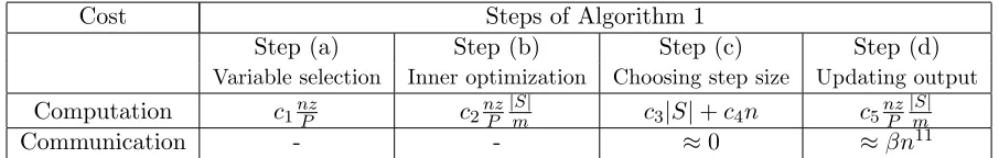
and the number of variables updated in each iteration respectively. To keep the analysis simple, we make the homogeneity assumption that the number of non-zero data elements in each node is nz/P. Let β( 1) be the relative computation to communication speed in the given distributed system; more precisely, it is the ratio of the times associated with communicating a floating point number and performing one floating point operation. On a cluster with 10 Gbps communication bandwidth where we did our experiments, we found the value of β to be in the range 30−100. Recall that n,m and P denote the number of examples, features and nodes respectively. Table 5 gives cost expressions for different steps of the algorithm in one outer iteration. Here c1, c2, c3, c4 and c5 are method dependent parameters. Table 5 gives the cost constants for various methods.We briefly discuss different costs below.
Cost Steps of Algorithm 1
Step (a) Step (b) Step (c) Step (d) Variable selection Inner optimization Choosing step size Updating output
Computation c1nzP c2nzP |mS| c3|S|+c4n c5nzP |mS|
Communication - - ≈0 ≈βn11
Table 2: Cost of various steps of Algorithm 1. Ccomp andP Ccomm are respectively, theP
sums of costs in the computation and communication rows.
Method c1 c2 c3 c4 c5 Computation Communication cost per iteration cost per iteration Existing methods
HYDRA 0 1 1 0 1 2nzP
|S|
m +|S| βn
GROCK 1 q 1 0 q nzP + 2qnzP |mS|+|S| βn
FPA 1 q 1 1 q nzP + 2qnzP |mS|+|S|+n βn
PCD 0 1 τls τls 1 2nzP |mS|+τls|S|+τlsn βn
Variations of our method
PCD-S 1 q τls τls q nzP + 2qnzP |mS|+τls|S|+τlsn βn
DBCD-R 0 k τls τls 1 (k+ 1)nzP
|S|
m +τls|S|+τlsn βn
DBCD-S 1 kq τls τls q nzP +q(k+ 1)nzP
|S|
m +τls|S|+τlsn βn
Table 3: Cost parameter values and costs for different methods. qlies in the range: 1≤q≤
m
|S|. R and S refer to variable selection schemes for step (a); see subsection 4.1.
PCDuses theRscheme and so it can also be referred to asPCD-R. Typicallyτls,
the number of α values tried in line search, is very small; in our experiments we found that on average it is not more than 10. Therefore all methods have pretty much the same communication cost per iteration.
Step a: Methods like ourDBCD-S12,GROCK,FPA andPCD-S need to calculate the gradient and model update to determine which variables to update. Hence, they need to go through the whole data once (c1 = 1). On the other hand HYDRA, PCD and DBCD-R select variables randomly or in a cyclic order. As a result variable subset selection cost is negligible for them (c1 = 0).
11. Note that the communication latency cost (the time taken to communicate zero bytes) is ignored in the communication cost expressions because it is dominated by the throughput cost for largen. Moreover, as in Agarwal et al. (2013), the broadcast and reduce operators are pipelined over the vector entries. This means that communication cost increases sub-linearly wrt. logP. Ifnis assumed to be large (as in our case), it is almost independent oflogP and can be written approximately asβn.
Step b: All the methods except DBCD-S and DBCD-R use the decoupled quadratic approximation (4). For DBCD-R and DBCD-S, an additional factor of k comes in c2 since we dokinner cycles of CDNin each iteration. HYDRA,PCD and DBCD-R do a random or cyclic selection of variables. Hence, a factor of |mS| comes in the cost since only a subset |S| of variables is updated in each iteration. However, methods that do selection of variables based on the magnitude of update or expected objective function decrease (DBCD-S, GROCK,FPA and PCD-S) favour variables with low sparsity. As a result, c2 for these methods has an additional factorq where 1≤q ≤ |mS|.
Step c: For methods that do not use line-search, c3 = 1 andc4 = 013. The overall cost is |S|to update the variables. For methods likeDBCD-S,DBCD-R,PCD andPCD-S that do line-search,c3 =c4 =τlswhereτls is the average number of steps (α values tried) in one
line search. For each line search step, we need to recompute the loss function which involves going over nexamples once. Moreover, AllReduce step needs to be performed to sum over the distributed l1 regularizer term. Since only one scalar needs to be communicated per line search step, the communication cost is dominated by the communication latency, i.e. the time taken to communicate zero bytes. As pointed out in Bian et al. (2013), τls can
increase with P; but it is still negligible compared ton. Combined with the fact thatn is large in step (d), we will ignore this cost in the subsequent analysis.
Step d: This step involves computing and doingAllReduce on updated local predictions to get the global prediction vector for the next iteration and is common for all the methods. Note that because we are dealing with linear models, the updated predictions need to be communicated only once in each iteration even for the methods like ours that require line search, i.e., there is no need to communicate the updated predictions again and again for every line search step in each iteration.
The analysis given above is only forCP
comp andCcomm, the computation and communi-P cation costs in one iteration. IfTP is the number of iterations to reach a certain optimality tolerance, then the total cost of Algorithm 1 is: CP =TP(Ccomp +P Ccomm). ForP P nodes, speed-up is given byC1/CP. To illustrate the ill-effects of communication cost, let us take
the method of Richt´arik and Tak´aˇc (2015). For illustration, take the case of |S|=P, i.e., one variable is updated per node per iteration. For large P, CP ≈ TPCcomm =P TP βn; bothβ andnare large in the distributed setting. On the other hand, forP = 1,CP
comm = 0 andCP =CP
comp ≈ nzm. Thus speedup = T1 TP
C1 CP =
T1 TP
nz m
βn. Richt´arik and Tak´aˇc (2015)
show that T1/TP increases nicely withP. But, the term βnin the denominator ofC1/CP
has a severe detrimental effect. Unless a special distributed system with efficient commu-nication is used, speed up has to necessarily suffer. When the training data is huge and so the data is forced to reside in distributed nodes,the right question to ask is not whether we get great speed up, but to ask which method is the fastest. Given this, we ask how various choices in the steps of Algorithm 1 can be made to decreaseCP. Suppose we devise choices such that (a)Ccomp is increased while still remaining in the zone whereP CcompP Ccomm,P
and (b) in the process,TP is decreased greatly, thenCP can be decreased. The basic idea of our method is to use a more complexfpt than the simple quadratic in (4), due to which,
TP becomes much smaller. The use of line search,(c.3)for stepcaids this further. We see
in table 5 that, DBCD-R and DBCD-S have the maximum computational cost. On the other hand, communication cost is more or less the same for all the methods (except for few scalars in the line search step) and dominates the cost. In section 6, we will see on various datasets how, by doing more computation, our methods reduce TP substantially over the other methods while incurring a small computation overhead (relative to communication) per iteration. These will become amply clear in section 6; see, for example, table 6.3 in that section.
6. Experimental Evaluation
In this section, we present experimental results on real-world datasets for the training of
l1 regularized linear classifiers using the squared hinge loss. Here training refers to the minimization of the function F in (1). We compare our methods with several state of the art methods, in particular, those analyzed in section 5 (see the methods in the first column of table 5) together with ADMM, the accelerated alternating direction method of multipliers (Goldstein et al., 2014). To the best of our knowledge, such a detailed study has not been done for parallel and distributedl1 regularized solutions in terms of (a) accuracy and solution optimality performance, (b) variable selection schemes, (c) computation versus communication time and (d) solution sparsity. The results demonstrate the effectiveness of our methods in terms of total (computation + communication) time on both accuracy and objective function measures.
6.1 Experimental Setup
Datasets: We conducted our experiments on four datasets: KDD,URL,ADSand WEB-SPAM14. The key properties of these datasets are given in table 6.1. These datasets have a large number of features and l1 regularization is important. The number of examples is large forKDD,URLand ADS.WEBSPAMhas a much smaller number of examples and hence communication costs are low for this dataset.
Dataset n m nz s=nz/m
KDD 8.41×10⁶ 20.21×10⁶ 0.31×10⁹ 15.34 URL 2.00×10⁶ 3.23×10⁶ 0.22×10⁹ 68.11 ADS 18.56×10⁶ 0.20×10⁶ 5.88×10⁹ 29966.83 WEBSPAM 0.26×10⁶ 16.60×10⁶ 0.98×10⁹ 58.91
Table 4: Properties of datasets. nis the number of examples, mis the number of features,
nz is the number of non-zero elements in the data matrix, and s is the average number of non-zero elements per feature.
Methods and Metrics: We evaluate the performance of all the methods using (a) Area Under Precision-Recall Curve (AUPRC) (Sonnenburg and Franc, 2010; Agarwal et al.,
2013)15 and (b) Relative Function Value Difference (RFVD) as a function of time taken. RFVD is computed as F(wFt)∗−F∗ where F∗ is taken as the best value obtained across the
methods after a long duration. We also report per node computation time statistics and sparsity pattern behavior of all the methods.
Parameter Settings: For each dataset we used cross validation to find the optimal λ
value that gave the best AUPRC values. For each dataset we experimented with a range of λ values centred around the optimal value that have good sparsity variations over the optimal solution. Since the relative performance between methods was quite consistent across different λ values, we give details of the performance only for the optimal λ value. With respect to algorithm 1, the working set size (WSS) per node and the number of nodes (P) are common across all the methods. We set WSS in terms of the fraction (r) of the number of features per node, i.e., WSS=rm/P. Note that WSS will change with P for a given fractionr. For all datasets we give results for tworvalues (0.01,0.1). Note thatrdoes not play a role in ADMM since all variables are optimized in each node. We experimented with P = 25,100. Only for ADS dataset we used P = 100,200 because it has many more examples than others.
Platform: We ran all our experiments on a Hadoop cluster with 379 nodes and 10 Gbit interconnect speed. Each node has Intel (R) Xeon (R) E5-2450L (2 processors) running at 1.8 GHz and 192 GB RAM. (Though the datasets can fit in this memory configuration, our intention is to test the performance in a distributed setting.) All our implementations were done inC# including our binary treeAllReduce support (Agarwal et al., 2013) on Hadoop. We implemented the pipelinedAllReduce operation described in Agarwal et al. (2013) that reduces the communication cost fromβnlogP toβnfor largen.
6.2 Method Specific Parameter Settings
We discuss method specific parameter setting used in our experiments and associated prac-tical implications.
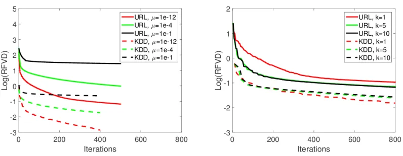
Choice of µ and k for DBCD: To get a practical implementation that gives good per-formance in our method, we deviate slightly from the conditions of Theorem 1. First, we find that the proximal term does not contribute usefully to the progress of the algorithm (see the left side plot in figure 1). So we choose to set µ to a small value, e.g.,µ= 10−12. Second, we replace the stopping condition (11) by simply using a fixed number of cycles of coordinate descent to minimizeft
p. The right side plot in figure 1 shows the effect of number
of cycles,k. We found that k= 5,10 are good choices. Since computations are heavier for DBCD-S, we usedk= 5 for it and usedk= 10 forDBCD-R.
Let us begin with ADMM. We use the feature partitioning formulation of ADMM described in subsection 8.3 of Boyd et al. (2011). ADMM does not fit into the format of algorithm 1, but the communication cost per outer iteration is comparable to the other methods that fit into algorithm 1. In ADMM, the augmented Lagrangian parameter (ρ) plays an important role in getting good performance. In particular, the number of iterations required by ADMM for convergence is very sensitive with respect toρ. While many schemes have been discussed in the literature (Boyd et al., 2011) we found that selecting ρ using the objective function value gave a good estimate; we selected ρ∗ from a handful of ρ
Figure 1: Study ofµ and k on KDD and URL. Left: the effect of µ. Right: the effect of k, the number of cycles to minimizeft
p. µ= 10−12 andk= 10 are good choices. P= 100.
values with ADMM run for 10 iterations (i.e., not full training) for each ρ value tried.16 However, this step incurred some computational/communication time. Note that each ADMM iteration optimizes all variables and involves many inner iterations, thus causing even the ten iterations each for several ρ values to be significantly large. In our time plots shown later, the late start of ADMM results is due to this cost. Note that this minimal number of ten iterations was essential to get a decentρ∗.
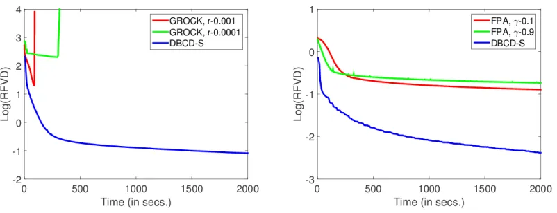
Now consider GROCK, FPA and HYDRA which are based on using Lipschitz con-stants (Lj). We foundGROCKto be either unstable and diverging or extremely slow. The left side plot in figure 2 depicts these behaviors. The solid red line shows the divergence case. FPA requires an additional parameter (γ) setting for the stochastic approximation step size rule. Our experience is that setting right values for these parameters to get good performance can be tricky and highly dataset dependent. The right side plot in figure 2 shows the extremely slow convergence behavior of FPA; its objective function also shows a non-monotone behavior. Therefore, we do not include GROCKand FPAfurther in our study.
For HYDRA we tuned Lj as follows. We set the first value of Lj to the theoretical
default value proposed in Richt´arik and Tak´aˇc (2016) and decreased it by a factor ofβ = 2 each time to create five values for Lj. Then we ran 25 iterations of HYDRA for each of those five values to chose the best value for Lj and then used that value for all remaining
iterations. We found that this simple procedure was sufficient to arrive at a near-best single value for Lj. Unlike ADMM, the cost of this tuning step is negligible compared to the
overall cost. Richt´arik, and Tak´aˇc (Richt´arik and Tak´aˇc, 2016) also showed results with the asynchronous implementation. For fair comparison with other synchronous approaches, we show results with the synchronous implementation only. Extending our work to the asynchronous setting and comparing with the asynchronous variants of other algorithms is an interesting future work.
Figure 2: Left: Divergence and slow convergence ofGROCKon theURLdataset (λ= 2.4×10⁻⁶ and P = 25). Right: Extremely slow convergence of FPA on theKDD dataset (λ= 4.6×10⁻⁷ andP = 100).
6.3 Performance Evaluation
We begin by comparing the efficiency of various methods and demonstrating the superiority of the new methods that were developed in section 4 and motivated in section 5. After this we analyze and explain the reasons for the superiority.
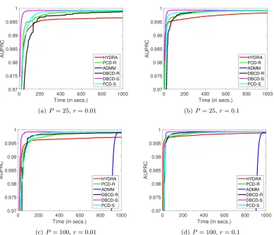
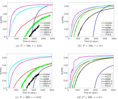
Study on AUPRC and RFVD: We have compared the performance of all methods by studying the variation of AUPRC and RFVD as a function of time, for various choices ofλ,
r (note that r defines the working set size, WSS=rm/P) and the number of nodes (P). To avoid cluttering with too many plots, we provide only representative ones - for each dataset, we choose one value forλand two values each, for r and P.
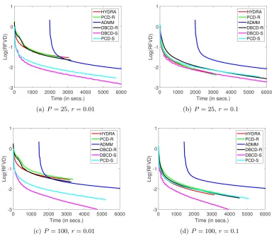
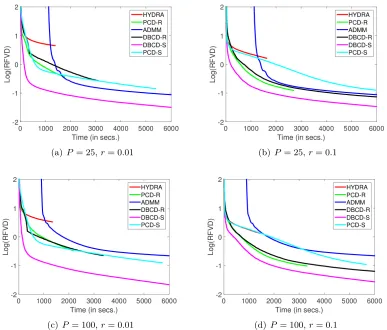
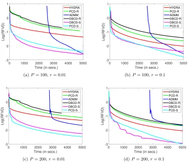
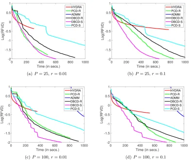
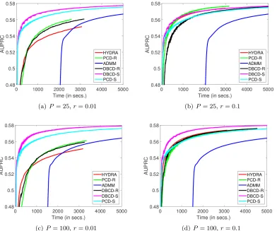
Figures 3-6 show the RFVD versus time plots for the four datasets; note the use of log scale for RFVD in those plots. Figures 7-10 show the AUPRC versus time plots. The following observations can be made from these plots.
Superior performance of DBCD-S. In most casesDBCD-S is the best performer. In several of these cases,DBCD-Sbeats other methods very clearly; for example, onURL withP = 100 andr = 0.01 (see the bottom left plot of figure 4), the time needed to reach log RFVD=-0.5 is many times smaller than any other method. As another example, with KDD and r = 0.01 (see the left side plots in figure 3), if we set the log RFVD value to −2 as the stopping criterion, DBCD-S and PCD-S are faster than all other methods by an order of magnitude. Even in cases where DBCD-Sis not the best (e.g., the case in the bottom left plot of figure 5), DBCD-Sperforms quite close to the best method.
How good is PCD-S? Recall from subsection 4.5 that PCD-S is the variation of the PCDN method Bian et al. (2013) using the S-scheme for variable selection. In some cases such as the last one pointed out in the previous paragraph,PCD-Sgives an excellent performance. However, in many other cases,PCD-Sdoes not perform well. This shows that working with quadratic approximations (like PCD-Sdoes) can be quite inferior compared to using the actual nonlinear objective like DBCD-Sdoes.
PCD-R), Only onWEBSPAM,PCD-R does slightly better than PCD-Sin some cases. One possible reason for this is that WEBSPAMhas a small number of examples, causing the communication cost to be much lower than the computation cost; note that the S-scheme requires more computation than the R-scheme.
Effect of r. The choice of r has an effect on the speed of various methods. But the sensitivity is not great. ForDBCD-S, a reasonable choice is r= 0.1.
Performance of HYDRA. Though HYDRA has a good rate of descent in the ob-jective function during the very early stages, it becomes quite slow soon after, leading to inferior performance. This shows up clearly even in the AUPRC plots.
Performance of ADMM. First note that ADMM is independent of r since all the variables are updated. ADMM has a late start due to the time needed for tuning the augmented lagrangian parameter, ρ. (In some cases - see the top two plots in figure 6 - the ADMM curves are not even visible due to the initial tuning cost being relatively large.) Unfortunately, this tuning step is unavoidable; without it, ADMM’s performance will be adversely affected. In many cases, DBCD-S reaches excellent solution accuracies even beforeADMM begins making any progress.
Consistency between RFVD and AUPRC plots. On KDD, URL and ADS datasets there is good consistency between the two sets of plots. For example, the clear superiority ofDBCD-Sseen in the top left RFVD plot of figure 4 is also seen in the top left AUPRC plot of figure 8. Only onWEBSPAM (see figure 6 and figure 10) the two sets of plots have some inconsistency; in particular, note that, in figure 6, the initial decrease of the objective function is faster forHYDRAthanDBCD-S, while, in figure 10,DBCD-Sshows better initial increase in AUPRC than HYDRA. This happens because DBCD-S makes many more variables non-zero and touches many more examples thanHYDRAin the initial steps.
Overall, the results point to the choice ofDBCD-Sas the preferred method as it is highly effective with an order of magnitude improvement over existing methods in many cases. Let us now analyze the reason behind the superior performance of DBCD-S. It is very much along the motivational ideas laid out in section 5: since communication cost dominates computation cost in each outer iteration, DBCD-Sreduces overall time by decreasing the number of outer iterations.
Study on the number of outer iterations: We study TP, the number of outer iter-ations needed to reach log RFVD≤ τ. Table 6.3 gives TP values for various methods in various settings. DBCD-S clearly outperforms other methods in terms of having much smaller values for TP. PCD-S is the second best method, followed by ADMM. The solid reduction ofTP by DBCD-Svalidates the design that was motivated in section 5. The in-creased computation associated with DBCD-Sis immaterial; because communication cost overshadows computation cost in each iteration for all methods, DBCD-Sis also the best in terms of the overall computing time. The next set of results gives the details.
(a)P = 25,r= 0.01 (b) P= 25,r= 0.1
(c)P = 100,r= 0.01 (d) P= 100,r= 0.1
Figure 3: KDD dataset. Relative function value difference in log scale. λ= 4.6×10⁻⁷
and 10 inner iterations. PCD-RandPCD-Stake a little more time thanHYDRAbecause of the line search. As seen in bothDBCD and PCDcases, a marginal increase in time is incurred due to the variable selection cost with the S-scheme compared to the R-scheme.
(a)P = 25,r= 0.01 (b) P= 25,r= 0.1
(c)P = 100,r= 0.01 (d) P= 100,r= 0.1
Figure 4: URLdataset. Relative function value difference in log scale. λ= 9.0×10⁻⁸
and gives an excellent order of magnitude improvement in overall time. With the additional benefit provided by the S-scheme, DBCD-S clearly turns out to be the method of choice for the distributed setting.
The methods considered in this paper are all synchronous methods. Also, asl1-regularization gives sparse solutions, load balancing can be prominent and lead to the “curse of last re-ducer” issue. The increase in waiting time (in our measurement, waiting time is counted as a part of the communication time) is higher for methods that involve greater computation; this is clear from table 6.3 where, roughly, communication time per iteration is higher for methods with higher computation time per iteration. In spite of this, our DBCD-S method, which has the largest computation and communication times per iteration, wins because of the drastically reduced number of iterations compared to other methods.
(a) P= 100,r= 0.01 (b)P = 100,r= 0.1
(c)P = 200,r= 0.01 (d) P= 200,r= 0.1
Figure 5: ADSdataset. Relative function value difference in log scale. λ= 2.65×10⁻⁶.
It is interesting to note that such an initial behavior seems necessary to make good progress in terms of both function value and AUPRC. In all the cases, many variables stay at zero after initial iterations; therefore, shrinking ideas (i.e., do not consider for selection those variables that tend to remain at zero) can be used to improve efficiency.
Remark on Speed up: Let us consider the RFVD plots corresponding to DBCD-S in figures 3 and 4. It can be observed that the times associated withP = 25 and P = 100 for reaching a certain tolerance, say log RFVD=-2, are close to each other. This means that using 100 nodes gives almost no speed up over 25 nodes, which may prompt the question:
Is a distributed solution really necessary? There are two answers to this question. First, as we already mentioned, when the training data is huge17 and so the data is generated and forced to reside in distributed nodes, the right question to ask is not whether we get great speed up, but to ask which method is the fastest. Second, for a given dataset, if the time taken to reach a certain optimality tolerance is plotted as a function of P, it may have a minimum at a value different from P = 1. In such a case, it is appropriate to choose a P (as well as r) optimally to minimize training time. Many applications involve
(a)P = 25,r= 0.01 (b) P= 25,r= 0.1
(c)P = 100,r= 0.01 (d) P= 100,r= 0.1
Figure 6: WEBSPAMdataset. Relative function value difference in log scale. λ= 3.92×10⁻⁵
periodically repeated model training. For example, in Advertising, logistic regression based click probability models are retrained on a daily basis on incrementally varying datasets. In such scenarios it is worthwhile to spend time to tune parameters such as P and r in an early deployment phase to minimize time, and then use these parameter values for future runs.
It is also important to point out that the above discussion is relevant to distributed settings in which communication causes a bottleneck. If communication cost is not heavy, e.g., when the number of examples is not large and/or communication is inexpensive such as in multicore solution, then good speed ups are possible; see, for example, the results in Richt´arik and Tak´aˇc (2015).
7. Recommended DBCD algorithm
Algorithm 2:Recommended DBCD algorithm
Parameters: Proximal constant µ >0 (Default: µ= 10−12);
WSS = # variables to choose for updating per node (Default: WSS=r m/P,r= 0.1);
k= # CD iterations to use for solving (3) (Default: k= 10); Line search constants: β, σ∈(0,1) (Default: β= 0.5, σ= 0.01); Choose w0 and computey0=Xw0;
for t= 0,1. . .do
forp= 1, . . . , P (in parallel) do
(a) For eachj∈Bp, solve (5) to get qj. Sort{qj :j∈Bp} and choose WSS
indices with leastqj values to form Spt;
(b) Formfpt(wBp) using (6) and solve (3) usingk CD iterations to get ¯wBpt
and set direction: dtBp = ¯wtBp−wBpt ; (c) Computeδyt=P
pXBpdtBp using AllReduce;
(d)α= 1;
while(12-13) are not satisfied do α←αβ;
Check (12)-(13) usingy+α δy and aggregating thel1 regularization value via AllReduce;
ende
Setαt=α,wtBp+1=wBpt +αtdtBp and yt+1=yt+αtδyt; endf
(a)P = 25,r= 0.01 (b) P= 25,r= 0.1
(c)P = 100,r= 0.01 (d) P= 100,r= 0.1
Figure 7: KDDdataset. AUPRC Plots. λ= 4.6×10⁻⁷
8. Conclusion
In this paper we have proposed a class of efficient block coordinate methods for the dis-tributed training of l1 regularized linear classifiers. In particular, the proximal-Jacobi ap-proximation together with a distributed greedy scheme for variable selection came out as a strong performer. There are several useful directions for the future. It would be useful to explore other approximations such as block GLMNET and block L-BFGSsuggested in subsection 4.2. Like Richt´arik and Tak´aˇc (2015), developing a complexity theory for our method that sheds insight on the effect of various parameters (e.g., P) on the number of iterations to reach a specified optimality tolerance is worthwhile. It is possible to extend our method to non-convex problems, e.g., deep net training, which has great value.
Proof of Theorem 1
First let us write δj in (11) as δj = Ejjdtj where Ejj =δj/(dtBp)j. Note that |Ejj| ≤µ/2.
(a)P = 25,r= 0.01 (b) P= 25,r= 0.1
(c)P = 100,r= 0.01 (d) P= 100,r= 0.1
Figure 8: URLdataset. AUPRC plots. λ= 9.0×10⁻⁸
with the gradient consistency property of Condition 1 to get
gStt p+H
t St
pd t St
p+ξSpt = 0, (15)
whereHStt
p = ˆHSpt−ESpt and ˆHSpt is the diagonal submatrix of ˆH corresponding toS t p. Since
ˆ
H≥µI and |Ejj| ≤µ/2, we getHStt p ≥
µ
2I. Let us extend the diagonal matrix E
t St
p toEBp
by defining Ejj = 0∀j∈Bp\Spt. This lets us extendHStt
p toHBp via H t
Bp = ˆHBp−EBp.
Now (15) is the optimality condition for the quadratic minimization,
dtBp = arg min
dBp
(gtBp)TdBp+
1 2(dBp)
TH
BpdBp+
X
j∈Bp
λ|wt
(a) P= 100,r= 0.01 (b)P = 100,r= 0.1
(c)P = 200,r= 0.01 (d) P= 200,r= 0.1
Figure 9: ADSdataset. AUPRC Plots. λ= 2.65×10⁻⁶
Combined over allp,
dt= arg min
d (g
t)Td+1
2d
THd+u(wt+d)
s.t. dj = 0∀j∈ ∪p(Bp\Spt) (17)
whereH is a block diagonal matrix with blocks,{HBp}. Thus dt corresponds to the
mini-mization of a positive definite quadratic form, exactly the type covered by the Tseng-Yun theory (Tseng and Yun, 2009).
The line search condition (12)-(13) is a special case of the line search condition in Tseng and Yun (2009). The Seidel scheme of subsection 4.1 is an instance of the Gauss-Seidel scheme of Tseng and Yun (2009). Now consider the distributed greedy scheme in subsection 4.1. Let jmax = arg max1≤j≤mq¯j. By the way the Spt are chosen, jmax ∈ ∪pSpt.
Therefore, P
j∈∪pSt pq¯j ≤
1
m
Pm
(a)P = 25,r= 0.01 (b) P= 25,r= 0.1
(c)P = 100,r= 0.01 (d) P= 100,r= 0.1
Figure 10: WEBSPAM dataset. AUPRC Plots. λ= 3.92×10⁻⁵. Because the initial ρ tuning time for ADMM is large, its curves are not seen in the shown time window of 0-100 secs.
References
A. Agarwal, O. Chapelle, M. Dudik, and J. Langford. A reliable effective terascale linear learning system. JMLR, 15:1111–1133, 2013.
Y. Bian, X. Li, and Y. Liu. Parallel coordinate descent Newton for large scale L1 regularized minimization. arXiv:1306.4080v1, 2013.
S. Boyd, N. Parikh, E. Chu, B. Peleato, and J. Eckstein. Distributed optimization and statistical learning via the alternating direction method of multipliers. Foundations and Trends in Machine Learning, pages 1–122, 2011.
J.K. Bradley, A. Kyrola, D. Bickson, and C. Guestrin. Parallel coordinate descent for
(a)r= 0.01 (b) r= 0.1
Figure 11: Per-node computation time on theKDDdataset (λ= 4.6×10⁻⁷ andP = 100).
(a)r= 0.01 (b) r= 0.1
Figure 12: KDDdataset: Typical behavior of the percentage of non-zero variables.
W. Deng and W. Yin. On the global and linear convergence of the generalized alternating direction method of multipliers. Journal of Scientific Computing, pages 889–916, 2016.
W. Deng, M-J. Lai, and W. Yin. On the o(1k) convergence and parallelization of the alternating direction method of multipliers. arXiv:1312.3040, 2013.
F. Facchinei, S. Sagratella, and G. Scutari. Flexible parallel algorithms for big data opti-mization. ICASSP, 2014.
J. H. Friedman, T. Hastie, and R. Tibshirani. Regularization paths for generalized linear models via coordinate descent. Journal of Statistical Software, 33:1–22, 2010.
M. Jaggi, V. Smith, M Tak´aˇc, J. Terhorst, S. Krishnan, T. Hofmann, and M.I. Jordan. Communication-efficient distributed dual coordinate ascent. NIPS, 2014.
M. Li, D.G. Andersen, J.W. Park, A.J. Smola, A. Ahmed, J. Josifovski, J. Long, E.J. Shekita, and B. Su. Scaling distributed machine learning with the parameter server.
OSDI, 2014.
C. Ma, V. Smith, M. Jaggi, M.I. Jordan, M Tak´aˇc, and P. Richt´arik. Adding vs. averaging in distributed primal-dual optimization. ICML, 2015.
I. Necoara and D. Clipici. Efficient parallel coordinate descent algorithm for convex opti-mization problems with separable constraints: application to distributed MPC. Journal of Process Control, 23:243–253, 2014.
Y. Nesterov. Efficiency of coordinate descent methods on huge-scale optimization problems.
SIAM Journal of Optimization, pages 341–362, 2012.
J. M. Ortega and W. C. Rheinboldt. Iterative solution of nonlinear equations in several variables. Academic Press, New York, 1970.
N. Parikh and S. Boyd. Block splitting of distributed optimization. Math. Prog. Comp., 2013.
M. Patriksson. Cost approximation: A unified framework of descent algorithms for nonlinear programs. SIAM J. Optim., 8:561–582, 1998a.
M. Patriksson. Decomposition methods for differentiable optimization problems over carte-sian product sets. Comput. Optim. Appl., 9:5–42, 1998b.
Z. Peng, M. Yan, and W. Yin. Parallel and distributed sparse optimization.IEEE Asilomar Conference on Signals, Systems, and Computers, 2013.
C. Ravazzi, S. M. Fosson, and E. Magli. Distributed soft thresholding for sparse signal recovery. Proceedings of IEEE Global Communications Conference, 2013.
P. Richt´arik and M Tak´aˇc. Iteration complexity of randomized block-coordinate descent methods for minimizing a composite function. Mathematical Programming, 144:1–38, 2014.
P. Richt´arik and M. Tak´aˇc. Parallel coordinate descent methods for big data optimization.
Mathematical Programming, 2015.
P. Richt´arik and M. Tak´aˇc. Distributed coordinate descent method for learning with big data. JMLR, 17:1–25, 2016.
C. Scherrer, M. Halappanavar, A. Tewari, and D. Haglin. Scaling up coordinate descent algorithms for largel1 regularization problems. ICML, pages 1407–1414, 2012a.
S. Shalev-Shwartz and A. Tewari. Stochastic methods for l1 regularized loss minimization.
JMLR, 12:1865–1892, 2011.
S. T. Sonnenburg and V. Franc. COFFIN: a computational framework for linear SVMs.
ICML, 2010.
P. Tseng and S. Yun. A coordinate gradient descent method for nonsmooth separable minimization. Mathematical Programming, 117:387–423, 2009.
G. X. Yuan, K. W. Chang, C. J. Hsieh, and C. J. Lin. A comparison of optimization methods and software for large-scale l1-regularized linear classification. JMLR, pages 3183–3234, 2010.
G. X. Yuan, C. H. Ho, and C. J. Lin. An improved GLMNET for L1-regularized logistic regression and support vector machines. JMLR, pages 1999–2030, 2012.
KDD, λ= 4.6×10⁻⁷
Existing methods Our methods
P τ HYDRA PCD-R PCD-S DBCD-R DBCD-S
−1 298 294 12 236 8
25 −2 >800 >800 331 >800 124
−3 >800 >800 >800 >800 688
−1 297 299 13 230 10
100 −2 >800 >800 311 >800 137
−3 >800 >800 >800 >800 797
URL,λ= 9.0×10⁻⁸
Existing methods Our methods
0 >2000 878 201 770 23
25 −0.5 >2000 >2000 929 1772 42
−1 >2000 >2000 >2000 >2000 216
0 >2000 840 197 476 27
100 −0.5 >2000 >2000 858 1488 55
−1 >2000 >2000 >2000 >2000 287
WEBSPAM, λ= 3.9×10⁻⁵
Existing methods Our methods
0 521 202 56 169 13
25 −0.5 >1500 185 109 128 25
−1.0 >1500 532 180 439 39
0 511 203 56 180 28
100 −0.5 >1500 308 111 265 49
−1.0 >1500 525 235 403 74
ADS, λ= 2.6×10⁻⁶
Existing methods Our methods
−1.0 573 >600 10 >600 7
100 −1.5 >600 >600 61 >600 18
−2.0 >600 >600 169 >600 53
−1.0 569 >600 10 >600 11
200 −1.5 >600 >600 35 >600 46
−2.0 >600 >600 154 >600 138
Table 5: TP, the number of outer iterations needed to reach log RFVD≤τ, for various P