Generalized Exp $\phi(\xi))$-expansion Method for Solving Non-linear Evolution Equations

Vol. 14, No. 3, 2017, 353-358

ISSN: 2279-087X (P), 2279-0888(online) Published on 10 October 2017

www.researchmathsci.org

DOI: http://dx.doi.org/10.22457/apam.v14n3a1

353

Annals of

Generalized Exp

(

ϕ

(

ξ

))

-expansion Method for Solving

Non-linear Evolution Equations

Md. Abdus Salam1 and Umme Habiba2

Department of Mathematics, Mawlana Bhashani Science and Technology University Tangail-1902, Bangladesh.

2

E-mail: [email protected]

Corresponding author. 1E-mail: [email protected] Received 19 August 2017; accepted 12 September 2017

Abstract. In this work, the generalized exp(

ϕ

(

ξ

))-expansion method is used to find traveling wave solutions of Korteweg-de Varies equation (KdV) and modified Liouville equation. This method gives travelling wave solutions and finally solitary wave solutions with respective graphs. The generalized exp(

ϕ

(

ξ

))−expansion method is very powerful and convenient mathematical tool for finding the exact solutions of nonlinear evolution equations arise in science and engineering.

Keywords: Generalized exp(

ϕ

(

ξ

))−expansion method; Korteweg-de Varies equation; Modified Liouville equation; Traveling wave solution; Solitary wave solution.

AMS Mathematics Subject Classification (2010): 35QXX 1. Introduction

Nonlinear evolution equations arise in many fields of sciences including physics, mechanics and material science. A lot of methods have been used to handle nonlinear evolution equations with constant coefficients and time dependent coefficients. Recently many effective methods for finding exact solutions of nonlinear evolution equations have been proposed, such as, the extended tan-method [1], enhanced

(

G /' G

)

− expansion method [2], modified Kudryashov method [3], exp-function method [4-5], exp(Φ(

ξ

)) -expansion method [6], F--expansion method [7], the Tanh method [8], Jacobi elliptic function rational expansion method [9], homotopy perturbation method [10], Modified simple equation method [11], the homogenous balance method [12], the variational method [13]. The objectives of this paper is to apply the generalized exp(

ϕ

(

ξ

))− expansion method for finding the exact traveling wave solutions of Korteweg-de Varies equation and modified Liouville equation which play an important role in mathematical physics.

354

2. Description of the generalised exp(

ϕ

(

ξ

))−expansion method

Suppose that a nonlinear partial differential equation, say in two independent variables x and t, is given byP(u,ut,ux,utt,uxt,uxx,LLL)=0, (2.1) where u=u( tx, ) is an unknown function, P is a polynomial in u=u(x,t) and its various partial derivatives, in which the highest order derivatives and nonlinear terms are involved. In the following the main steps of the exp(

ϕ

(

ξ

))−expansion method are given:

Step 1: The traveling wave variable u(x,t)=u(

ξ

) where

ξ

=x−ct permits us reducing eq. (2.1) to an ODE for u=u(

ξ

) in the form

, 0 ) ,

, , , , ,

(u −cu′ u′ c2u′′ −cu′′ u′′LLL =

P (2.2)

Step 2: Suppose the solution of eq. (2.2) can be expressed in the following form

i m

i i a

u( ) (exp( ( )))

0

ξ

ϕ

ξ

∑

=

= (2.3)

where a_i are constants, the positive integer m can be determined by considering the homogeneous balance between the highest order derivatives and the nonlinear terms appearing in eq. (2.2), and

ϕ

=

ϕ

(

ξ

) satisfies the following equations:

1 ,

0 )) ( (exp )

( ± = ' ≥

′

ξ

ϕ

ξ

n n

ϕ

(2.4) Equation (2.4) gives the following solutions of the forms:

[

( )

]

, 1

ln ) / 1 ( )

(

ξ

=− n ±n

ξ

+c₁ n≥

ϕ

(2.5)

Step 3: Now we substitute eq. (2.3) into eq. (2.2) and use eq. (2.4). As a result of this substitution, we get a polynomial of exp(

ϕ

(

ξ

))and equate the coefficients of exp(

ϕ

(

ξ

)) to zero. This procedure gives a system of algebraic equations which can be solved to find

0 1,...,

,a a

am m− .

Step 4: Putting the values of a_m,a_m−1,...,a₀ into eq. (2.3) along with general solutions of eq. (2.4) complete the determination of the solutions of eq. (2.1).

3. Applications of the generalized exp(

ϕ

(

ξ

))−expansion method

Now, we will apply the generalized exp(

ϕ

(

ξ

))−expansion method described in section 2 to find the exact traveling wave solutions of Korteweg-de Varies equation and modified Liouville equation.

Example 1. Solution of Korteweg-de Varies (KdV) equation

We know that the Korteweg-de Varies equation[14] is u_xxx−6uu_x+u_t =0 (3.1)

Suppose the traveling wave transformation is given by

Generalized Exp(

ϕ

(

ξ

))- expansion Method for Solving Non-linear Evolution Equations

355

where the prime denotes the differential with respect to

ξ

. The corresponding exact solutions of eq. (3.1) for different values of n are obtained below:

Case 1(n=1): Considering the homogeneous balance between u′′′and uu′rising in eq. (3.3), we get m=2. So from eq.(2.3) the solution can be written as

2 2

1

0 exp ( ) exp ( )

)

(

ξ

a a

ϕ

ξ

a

ϕ

ξ

u = + + (3.4)

where a0,a1,a2 are unknown constants to be determined and

ϕ

(

ξ

) satisfies the eq. (2.4)

and this function is determined from eq. (2.5) by setting n=1, Putting eq. (3.4) in the reduced ODE (3.3) and collecting the coefficients of exp(

ϕ

(

ξ

)), we get the system of algebraic equations. Solving these equations by using Maple-13, we get the values of constants: a₀ =(1/6)c,a₁ =0,a₂ =−2 .

Hence, the solution of eq. (3.3) takes the form: ₂

1 1 ) ( 2 6 ) (

ξ

ξ

± ± − = c c u

Finally, putting

ξ

=x−ct, we get the following desired exact solution of eq. (3.1)

2 1 1 )] ( [ 2 6 ) , ( ct x c c t x u − ± ± −

= (3.5)

Similarly, for n=2,3,4,.... the corresponding trail solution of the eq. (3.3), values of constants and exact solutions of eq. (3.1) are given below:

Case 2 (n=2): The trail solution of eq. (3.3):

4 4 3 3 2 2 1

0 exp( ( )) exp( ( )) exp( ( )) exp( ( ))

)

(

ξ

a a

ϕ

ξ

a

ϕ

ξ

a

ϕ

ξ

a

ϕ

ξ

u = + + + + (3.6)

Values of constants: a₀=(1/6)c,a₁ =0,a₂ =0,a₃ =0,a₄ =−8

The exact solution of eq.(3.1): ₂

1 2 )] ( 2 2 [ 8 6 ) , ( ct x c c t x u − ± ± −

= (3.7)

Case 3 (n=3): The trail solution of eq. (3.3):

6 6 5 5 4 4 3 3 2 2 1

0 exp( ( )) exp( ( )) exp( ( )) exp( ( )) exp( ( )) exp( ( ))

)

(ξ a a ϕξ a ϕξ a ϕξ a ϕξ a ϕξ a ϕξ

u = + + + + + + Values of constants: a0=(1/6)c,a1 =0,a2 =0,a3 =0,a4 =0,a5 =0,a6 =−18

The exact solution of eq. (3.1): ₂

1 3 )] ( 3 3 [ 18 6 ) , ( ct x c c t x u − ± ± −

= (3.8)

Case 4 (n=4): The trail solution of eq. (3.3):

)) ( exp( )) ( exp( )) ( exp( )) ( exp( )) ( exp( )) ( exp( )) ( exp( )) ( exp( ) ( 8 8 7 7 6 6 5 5 4 4 3 3 2 2 1 0 ξ ϕ ξ ϕ ξ ϕ ξ ϕ ξ ϕ ξ ϕ ξ ϕ ξ ϕ ξ a a a a a a a a a u + + + + + + + = (3.9)

Values of constants: a0=(1/6)c,a1=0,a2 =0,a3 =0,a4 =0,c,a6 =0,a7 =0,a8 =−32

The exact solution of eq. (3.1): ₂

1 4 )] ( 4 4 [ 32 6 ) , ( ct x c c t x u − ± ± −

356

In general, the exact solution of eq. (3.1): ₂

1 ( )]

[

) 1 ( 2 6

) , (

ct x n nc

n c

t x un

− ± ±

− −

=

Velocity profile of u₁(x,t) whenc=1

Fig.1(3d plot): profile of (10) for c₁=−10

Velocity profile of u₂(x,t) when c=2

Fig.2(3d plot): profile of (12) for c₁ =−20

Velocity profile of u3(x,t) whenc=3

Fig.3(3d plot): profile of (14) forc1=−100

Velocity profile of u4(x,t) whenc=4

Fig.4(3d plot): profile of (16) for c₁=−90 Figure 1-4: Graphical representation of Korteweg-de Varies (KdV) equation

The Figure 1 shows that the waves having high wave speed propagate with more height.

Example2. Solution of modified Liouville equation We know that the modified Liouville equation[15] is

w xx tt a w be

w = 2 + β (3.11) which is found in hydrodynamics, where w( tx, ) is the stream function and a,b,

β

are

nonzero constants. Let us consider that the transformation ( , ) w, e t x

u = β so that u

w=(1/

β

)ln (3.12) 0

2

3− ′ + ′′=

u u u

ku (3.13)

where

2 2

c a

b k

−

= β and c≠±a.For different values of n the solutions of eq. (3.11) are:

Case-1 (n=1): Solution is

[

]

















−

+

−

=

₂

1

2 2 1

)

(

)

(

2

ln

1

)

,

(

ct

x

c

b

a

c

t

x

w

β

Generalized Exp(

ϕ

(

ξ

))- expansion Method for Solving Non-linear Evolution Equations

357 Case-2 (n=2): Solution is

[

]

       − + − = 2 1 2 2 2 ) ( ) ( 2 ln 1 ) , ( ct x c b a c t x w

β

β

(3.15)

Case-3 (n=3) Solutionis

[

]

















−

+

−

=

₂ 1 2 2 3

)

(

)

(

2

ln

1

)

,

(

ct

x

c

b

a

c

t

x

w

β

β

(3.16)

Case-4 (n=4): Solution is

[

]

       − + − = ₂ 1 2 2 4 ) ( ) ( 2 ln 1 ) , ( ct x c b a c t x w

β

β

(3.17)

In general, the solution of eq. (3.11) is

[

]

       − + − = ₂ 1 2 2 ) ( ) ( 2 ln 1 ) , ( ct x c b a c t x w_n

β

β

(3.18)

From the above it is clear that the exact solutions of eq. (3.11) are same for all cases.

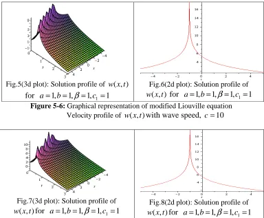
Fig.5(3d plot): Solution profile of w( tx, ) for a=1,b=1,

β

=1,c₁ =1

Fig.6(2d plot): Solution profile of )

, ( tx

w for a=1,b=1,

β

=1,c₁ =1 Figure 5-6: Graphical representation of modified Liouville equation

Velocity profile of w( tx, )with wave speed, c=10

Fig.7(3d plot): Solution profile of )

, ( tx

w for a=1,b=1,

β

=1,c1 =1

Fig.8(2d plot): Solution profile of )

, ( tx

w for a=1,b=1,

β

=1,c1=1 Figure 7-8: Velocity profile of w( tx, )with wave speed, c=11

4. Results and discussions

358

height of the wave is 0.49985 unit (approximate). When wave speed is 4, the height of the wave is 0.66660 unit (approximate). Again, from Fig. 5(3d plot) it is clear that the height of wave is 8 unit (approximate) for wave speed 10. Also for wave speed 11, from Fig. 7(3d plot) we see that the height of the wave is 10 unit. From the above discussion it is clear that the height of the wave increases with the increase of wave speed.

5. Conclusion

We can say that this method has capacity to minimize the size of computational work compared to other existing techniques. It removes complexity to get new solutions of non-linear evolution equations.

Acknowledgements. The authors gratefully acknowledge the financial support provided by research cell, Mawlana Bhashani Science and Technology University.

REFERENCES

1. M.A.Abdou, The extended tan-method and its applications for solving nonlinear physical model, Applied Mathematics and Computation, 190 (2007) 988-996. 2. M.E.Islam, K.Khan, M.A.Akbar and R.Islam, Travelling wave solutions of nonlinear

evolution equation via enhanced

(

G /′ G

)

−expansion method, GANIT, 33 (2013) 83-92.

3. M.M.Kabir, Modified Kudryashov Method for Generalized forms of the Nonlinear Heat Conduction Equation, Int. Journal of the Phy. Sci., 6(25) (2011) 6061-6064. 4. A.Khalid, Abdul Zahra and A. Mudhir, Abdul Hussain, Exp-function method for

solving nonlinear beam equation, Int. Math. Forum, 6 (2011) 2349-2359.

5. A.Bekir and A.Boz, Exact solutions for nonlinear evolution equation using exp function method, Physics Letters A, 372 (2008) 1619–1625.

6. K.Khan, and M.A.Akbar, Application ofExp(Φ(

ξ

))−expansion method to find the exact solutions of modified benjamin-bona-mahony equation, World Applied Science Journal, 24(10) (2013) 1373-1377.

7. M.S.Islam, K.Khan, M.Ali Akbar and A.Mastroberardino, A note on improved f-expansion method combined with Riccati equation applied to nonlinear evolution equations, Royal Society Open Science, (2014). DOI: 10.1098/rsos.140038

8. A.M.Wazwaz, The tanh method for travelling wave solutions to the Zhiber-shabat equation and other related equations, Communicationbs in Nonlinear Science and Numerical Simulation, 13 (2008) 584-592.

9. A.T.Ali, New generalized Jacobi elliptic function rational expansion method, J Comput Appl Math, 235 (2011) 4117–27.

10. J.H.He, Application of homotopy perturbation method to nonlinear wave equations, Chaos, Solitons and Fractals. 26 (3) (2005) 695–700.

11. A.J.M.Jawad, M.D.Petkovi´c and A.Biswas, Modified simple equation method for nonlinear evolution equations, App. Math. and Compu., 217(2) (2010) 869–877. 12. J.Weiss, M.Tabor and G.Carnevale, The Painleve property for partial differential

equations, J Math Phys, 24 (1983) 522.

Generalized Exp(

ϕ

(

ξ

))- expansion Method for Solving Non-linear Evolution Equations

359

14. M.Wadati, The exact solution of the modified Korteweg–de Vries equation, Journal of Physical Society of Japan, 32 (1972) 1681–1681.