w w w . i j m r e t . o r g I S S N : 2 4 5 6 - 5 6 2 8
Page 45
Evolutionary Optimization Using Big Data from Engineering
Simulations and Apache Spark
Sunil Suram
*Senior Data Scientist
Abstract: This paper presentsa novel data flow architecturethat utilizes data from engineering simulations to generate a reduced order model within Apache Spark. The reduced order model from Spark is then utilized by anevolutionary algorithm in the optimization of an industrial system component. This work is presented in the context of the shape optimization of a heat exchanger fin and demonstrates the ability of theengineering simulation, the reduced order model and the evolutionary algorithm to exchange data with each other by utilizing Spark as the common data-processing framework. In order to enable a user to monitor the input design parameter space,self-organizing maps are generated for visualization. The results of theevolutionary optimization utilizing this data flow are compared with results from invoking high-fidelity engineering simulations. This novel data flow architecture decouples the evolutionary algorithm from the reduced order model and allows improvement of the optimization results by continuously augmenting the reduced order model with data from the evolutionary algorithm.Additionally, when constraints on the optimization algorithm are modifiedthe evolutionary algorithm canadapt and evolve good solutions. Themethodology presented in this articlealso makes it feasible to simultaneously tune evolutionary optimization experiments along with engineering simulations at a relatively low computational cost.
Keywords: Engineering optimization; Evolutionary algorithms;Big Data, Apache Spark;Self-organizing maps; Engineering simulation data
I. Introduction
Evolutionary algorithms (EAs) are an established technique to solve engineering design and optimization problems when the search space is discontinuous and the design variables cannot be parameterized (Ashlock, 2006). When the fitness function is multi-modal, EAs are efficient at finding globally optimal solutions due to their stochastic nature (Liu et al. 2015; Ashlock, 2006; Deb, 2001; Holland, 1992). EAs have been utilized successfully for solving various engineering problems including inverse design (Liu, 2015) and design optimization problems(Ly, 2001; Suram, 2008; Yepes, 2017;Xu, 2016). However, there are several instances where the fitness function evaluation for engineering problems is time-consuming and computationally expensive, especially when engineering simulations have to be run to evaluate fitness values. Examples of engineering simulations includemethods like the finite element method, computational fluid dynamics, or other multi-physics based techniques. The results from complex engineering simulations are utilized by engineers to synthesize and design products while considering user requirements. However, the complexity and the time-consumingnature of simulations make it challenging for them to be used in an engineering design
optimization process. This causes engineering design optimization to be performed towards the end of the design cycle making the optimization process linear. Any iterations to the design can thus become challenging and time-consuming (Ullman, 2009). In such cases, EAs become restrictive due to the need for a large number of fitness evaluations (Peremezhney, 2014; Suram, 2006; Lohan, 2015; Dolci, 2015).
w w w . i j m r e t . o r g I S S N : 2 4 5 6 - 5 6 2 8
Page 46
the validity range of a ROM and the investigation of ROM re-training. Liu et al. (2015) compared several inverse methods to design enclosed spaces and found that the POD based reduced order models in conjunction with a genetic algorithm was the most effective in finding global optima. Several other examples of utilizing POD based ROMs can be found in the literature (Xiao et al. 2015; Castellani et al. 2016; Ushijima et al. 2015; Reddy et al. 2017), where the researchers have reduced computational time to solve optimization and design problems. In the approaches studied in the literature, researchers have constructed the ROM prior to including it in an optimization process. This approach has two primary drawbacks:
a) Knowledge of the design space: It assumes that the design engineer has a thorough understanding of the design space and can focus the collection of datasnapshotsappropriately. For relatively simple problems, engineer insight can help focus the process of snapshot collection,however,this can be challenging in complex multi-parameter optimization problems. Using an inadequate ensemble matrix can result in directing the optimization algorithm towards a sub-optimal set of solutions. If the design parameter space changes, the ensemble matrix must be reconstructed and the optimization process re-started.Furthermore, in an evolutionary algorithm, since the population is initialized randomly it might be challenging to encompass the entire parameter space in the ROM. b) Tightly coupled optimization:Once the
ROM approximation is constructed, the optimization algorithm needs complete information of the ROM to perform evaluations of the fitnessfunction. Thus,afterthe optimization process begins, changes to the underlying ROM are not possible in real-time. Additionally, the optimization process must be restarted each time the ROM is updated since the ROM is embedded in the EA.
This article takes an approach towards integrating the data flow between the engineering simulation and optimization processes using Apache Spark. The integrationof data flow enables a dynamic coupling where data and results can be utilized to enhance the simulations as well as the results of the design optimization. The data from engineering simulations is stored in an Apache Spark DataFrame (Zaharia, 2016), andis utilized to create a data-driven reduced-order model (ROM)by leveraging the machine learning library MLlib within Spark (Meng, 2016), as described in Section 3. Fast computations of
time-consuming fitness function are performed by the ROM, thus mitigating performance bottlenecks in the EA. Additionally, after each generation in the EA, anengineering simulation is triggered with the best fitness chromosome in the population, thus enhancing the accuracy of the ROM. Self-organizing maps (SOM) enable visualization of the design parameter space during the evolution process, which produces a 2-dimensional output of the multi-dimensional design parameter space. The output from the SOM enablesa user to visualize the design parameter space, and manually trigger simulations as needed, that cover portions of the design space that have not been covered in the initial ROM training set. Thus, the ROM can be constructed in an incremental manner in lieu of attempting to create it in a comprehensive mannerprior tostarting the optimization process.
In summary, the past research has primarily involved “embedding” the ROM into the EA. Thus, when new simulation data is added the ROM has to be repeatedly re-computed and included in the EA to find a new optimal design. This multi-step processmakes it challenging to update the EA results based on newer simulation data. This article explores the use of Apache Spark to store, compute and update simulation data as well as ROMs to create a system that enablesdecoupling the EA from the ROM for greater flexibility. The novelty of this approach lies in the data-flow architecture that allows results from the EA to be seamlessly incorporated into the ROM. Thus, the ROM can be updated and enhanced without re-starting the EA process.
II. Background
This section briefly outlines the techniques utilized in this work viz. evolutionary optimization, reduced order models and self-organizing maps.
2.1. Evolutionary Algorithm based Optimization
w w w . i j m r e t . o r g I S S N : 2 4 5 6 - 5 6 2 8
Page 47
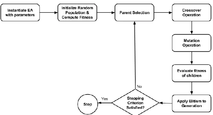
Figure (1). Flowchart of a generic evolutionary algorithm.
2.2. Reduced Order Models
Data-driven reduced order models are derived from computational data and are utilized in lieu of detailed computational models in order to reduce time to solution. ROMs are less accurate than the detailed high-fidelity computational models, but have the advantage of faster time to solution(Ly, 2001; Suram, 2008; Reddy 2017). Several ROM techniqueslike Krylov subspace, balanced truncation and proper orthogonal decomposition have been developed, studied, and applied successfully to several engineering problems. Proper orthogonal decomposition (POD) technique is utilized in this article and the remainder of this section describes the technique. The POD technique, also called principal components analysis (PCA), is based on the singular value decomposition (SVD) of a matrix. For a matrix A, which is also the training set on the available data, the SVD is defined as shown in Equation (1).
A = USVT (1)
The orthogonal matrices U and Vconstitute the left and right eigenvectors respectively. The matrix S is a diagonal matrix of singular values arranged in descending order of magnitude. The magnitude of each singular value defines the relative importance of the corresponding eigenvector. This is an important property of the SVD technique that can be utilized to select dominant axes of eigenvectors onto which the matrix A can be projected. The left eigenvector matrix U is projected onto the original data matrix A to compute the coefficient matrix for the ROM, as shown in Equation (2).
C = UA (2)
Once the matrix of coefficient vectors C is computed, predictions for design parameters 𝒗 outside the training set are calculated by finding two coefficient vectors that encompass 𝒗 using a cosine similarity measure (Steinbach, 2000). Once the encompassing vectors 𝒗 𝑳 and 𝒗 𝑹 are found, the corresponding coefficient vectors 𝒄 𝑳 and 𝒄 𝑹 are
selected from the C matrix. An interpolated coefficient vector 𝒄 𝑷 is computed using as shownin Equation (3).
𝒄𝑷
= 𝒄 + (𝒄𝑳 − 𝒄𝑹 )𝑳
𝒗 − 𝒗 𝑳 (𝒗 𝑹− 𝒗 )𝑳
(3)
The coefficient vector 𝒄 𝑷 is multiplied with the left-eigenvector matrix to compute the final prediction 𝒑 as show
in Equation (4).
𝒑
= 𝒄 𝑼𝑷 𝑻 (4)
The SVD computation in Equation (1) is the most computationally expensive operation in this technique, and must be computed only when there is an update to the training data. An approximate ROM solution can be easily computed using Equations (3) and (4), both of which are computationally inexpensive operations. Thus, POD based ROM techniques are approximations computed from high-fidelity simulation data to reduce time to solution in lieu of computationally expensive simulations. Further details on the POD technique can be found in the literature (Kirby, 2000; Gunzburger, 2002).
In the context of this article, every time the matrix A gets updated with new simulation data the SVD can be re-computed using MLib and the coefficient matrix is updated according to Equation (2) and all subsequent ROM computation are performed with the updated coefficients.
2.3. Self-Organizing Maps to Update Input Space
w w w . i j m r e t . o r g I S S N : 2 4 5 6 - 5 6 2 8
Page 48
two or three-dimensional space (Stefanovic, 2011). SOMs have been utilized in this article to visualize the high-dimensional input parameter space in two-dimensions at various stages during the evolutionary optimization process. A SOM is produced with the input design parameters and the unified distance matrix representation of the SOM is utilized to study the distribution of the input space and is leveraged by the user to execute additional simulations. These simulations are inturn stored in Spark to augment the existing data. An example of a unified distance matrix is shown in Figure (2), where the SOM has been recomputed after an update to the design parameter space. The darker regions represent larger distances in the input space.
Before After
Figure (2). Update to the unified distance matrix with updates to input parameter space.
The addition of an additional design in the input space changes the distribution of the unified distance matrix. This can be confirmed by the reduction in the darkly shaded regions on the right. The dots in Figure (2) represent the design parameter vectors in two-dimensional space. Thus, on visual observation of the unified distance matrix, the user can understand the representation in the input space and can opt to augment the input parameter space with new simulation data. Additional details about the technique can be found in the literature (Stefanovic, 2011; Ritter, 1992).
III. Data Flow Architecture using Apache Spark
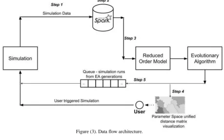
The sequence of steps starting from the results of the engineering simulation to the evolutionary optimization can be considered a series of successive transformations on data,and hence the overall architecture can be referred to as a data flow architecture. At each step, a transformation is appliedto the data from the previous step. The evolutionary algorithm finally utilizing the results from the ROM. Also, during the evolution process, elite chromosomes can be utilized to augment data used to create the ROM. This section describes the data flow architecture that has been developed utilizing Apache Spark, in detail, as shown in Figure (3).
w w w . i j m r e t . o r g I S S N : 2 4 5 6 - 5 6 2 8
Page 49
A key advantage of Apache Spark in this work is its ability to process data stored in a distributed file system. Engineering simulation data is generated and stored on a distributed file system and Apache Spark can compute the ROM without moving data to a separate cluster. The SVD computation is the most computationally expensive operation to create the ROM. Apache Spark utilizes the MLib library to perform a distributed SVD computation with all the engineering simulation data in place. It must be noted that this is an improvement from the methodologies discussed in prior research in this field where the simulation data has to be moved to a single node to construct the ROM.
At the beginning of the data flow, simulation data is stored in a Spark dataframe. In addition to the simulation data, the design parameters that define each simulation model are also stored in a separate dataframe within Spark. This information is utilized to compute the ROM (using Mllib) and the interpolation coefficients as described in Section (2). After the ROM is computed it can be used by the EA to evaluate the fitness of chromosomes in the population.Thus the data-flow approach decouples the construction of the ROM from the execution of the EA.
Itrequires the development of the following:
A process to enable adding engineering simulation data to a Spark dataframe.
A mechanism to trigger updates to the ROM based on new data. This also involves storing the updated A and U
matrices within Spark.
An EA process that can get updated ROM coefficients and eigen-vectors from Spark.
A process that can utilize the design parameter data and organize it using a SOM.
Step 1: Add Simulation Data to Spark
This is the first step in the data flow that transfers data from engineering simulations to a Spark cluster. This step of the data-flowmust have the ability to read data in the format emitted by the engineering simulation, connect to the Spark cluster and append the data to a specified dataframe or a resilient distributed dataset(RDD). In this article, the simulation computes temperature distribution data in comma separated value format which gets added to Spark.
Step 2: Compute SVD and ROM Coefficients
As soon as simulation data is updated from Step 1, the ROM needs to be recomputed so that the ROM coefficients and associated matrices can be updated to reflect changes to the data. This is accomplished by utilizingthe concept of a trigger in Apache Spark 2.2, i.e. specifically the ProcessingTimeAPI.The trigger allows the computation of the SVD, which is computed usingthe MLlib library in Spark, and atomically updates the dataframes that contain U
and A matrices on a periodic basis.
Step 3: Enable EA to read ROM coefficients and Umatrix
The updated ROM parameters and associated eigen-vectors must be utilized by the EA so that the optimization can continue with the latest updates to the underlying simulation data. At the completion of every generation, the EA updates its cached versions of the U and A matrices and thus has access to the latest ROM. It must be noted that there is a lag of one generation between the cached version of the ROM with the EA and the version in Spark. Also, any user triggered updates to the simulation data also get incorporated into the EA.
Step 4: Compute SOM of design parameters to visualize
Every time new simulation data is added, the input design parameter space also changes and the corresponding dataframe is updated. The SOM and the associated unified distance matrix are recomputed with the addition of new inputs for visualization and analysis by the user.
Step 5: Queue design parameters for simulations
In addition to the above steps, thebest chromosome from each generation of the EA isutilized to run anengineering simulation and append the generated data to Spark. This enables additional simulation datasets to be added without explicit user intervention and as the EA proceeds with optimization,the training dataset for ROM generation also gets augmented. The simulation solver is invoked asynchronously via a message queueing system.
Thus,the optimization, the numerical simulations and the ROM updates can occur independently,while each of these componentsis also seamlessly updating the outcomes of the other components. It should also be noted that in the case where the EA is invoking the ROM, the update frequency through the queue can be high and long simulation times can slow down the process of updating data to Spark and in turnfeedback to the ROM. In such cases, depending on the run time of the engineering simulation the EA can be paused for a brief period or the number of generations for evolution can be set to be large. This case is however not considered in this article.
The following section discusses in detail an engineering application that employs the developed Spark-based data flow architecture to optimize the shape of a heat-exchanger fin.
IV. Application and Results
w w w . i j m r e t . o r g I S S N : 2 4 5 6 - 5 6 2 8
Page 50
problem has been studied extensively in the literature and several references are available that discuss various aspects of heat-exchanger fin design (Incropera, 2002; Suram, 2006; Özisik, 1994).
4.1. Problem Description
In the example discussed in this article, a steady-state heat exchanger is considered where the fluid surrounding the fin is assumed to be air.The lateral surface of the fin can be curved and it extracts heat from a base plate. Some examples of heat-exchanger fins of varying profiles are shown in Figure (4). The geometry of the fin has been converted to non-dimensional form by dividing each dimension by the
length of the fin. Thus, the fin has unit length and all other dimensional parameters are less than one, which helps constrain the search space of the EA optimization. A two-dimensional system is considered and the engineering simulation of heat transfer in the fin at steady-state is performed by solving the governing partial-differential equations as shown in Equation (5a) and subject to the boundary conditions shown in Equations (5b-d),
where
n
is the surface normalalong the surface exposed to air and q is the heat flux.
𝜕2𝑇
𝜕𝑥2+
𝜕2𝑇
𝜕𝑦2= 0
(5a)
𝑘𝜕𝑇 𝜕𝑥 𝑙𝑒𝑓𝑡
= 𝑞
𝑘 𝜕𝑇 𝜕𝑛 𝑎𝑖𝑟 𝑏𝑑𝑟𝑦
= −ℎ 𝑇 − 𝑇𝑎𝑖𝑟
𝑘𝜕𝑇
𝜕𝑦 𝑙𝑜𝑤𝑒𝑟 = 0
(5b)
(5c) (5d)
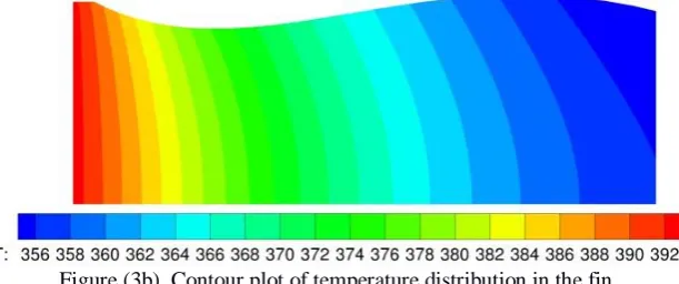
To simulate the temperature distribution in the heat-exchanger fin, the geometry of the heat-exchanger fin is discretized and the governing partial differential equations are solved using the finite-difference technique (Incropera, 2002). The number of grid points for simulation were chosen systematically by doubling the number of grid points until the change in the accuracy of the solution is negligible. The resulting grid dimensions are 401x401 grid resulting in approximately 161000 grid points. It must be noted that for problems involving coupled fluid dynamics and heat transfer the number of grid points can be higher. The techniques presented in this article can be applied to larger grid sizes from complex simulations. A contour plot of the temperature distribution in a representative fin is shown in Figure (3b), which shows a gradual decrease in the temperature along the x-axis since the heated surface is along the left boundary. The scale below the contour plot shows the temperature in degrees Celsius.
This engineering simulation code and the resulting data was utilized for optimization and to construct a ROM. Three types of fin profiles have been considered for optimization, i.e. 1st, 2nd and 4th degree polynomials. Each of these profiles are discussed in the context of the EA chromosomes in the next section.
Figure (3b). Contour plot of temperature distribution in the fin.
4.2. Chromosomes
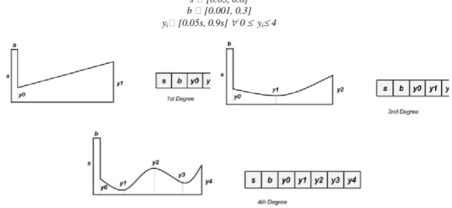
Figure (4) shows example shapes of each of the 1st, 2nd and 4th degree polynomial fin profiles and the structures of the corresponding chromosomes. The lengths of the chromosomes in each case are 4, 5, and 7 respectively. The larger chromosome lengths also represent a higher dimensional search space for the EA. Due to varying lengths of chromosomes, each shape design case is evolved independently. This also helps in maintaining diversity in the population by preventing the EA from selecting chromosomes from a higher-order shape dominating the population. In Figure (4), s represents the width of the heated base plate and b represents its thickness. The chromosome constitutes of distances along the y-axis,yiwhich are points on the curved surface of the fin that define the shape of its profile.
w w w . i j m r e t . o r g I S S N : 2 4 5 6 - 5 6 2 8
Page 51
and all the constraints are expressed in non-dimensional units. During fitness evaluation, if a chromosome does not respect these constraints, it is awarded a fitness value of zero thus penalizing the individual from progressing to the next generation.
s [0.05, 0.6] b [0.001, 0.3] yi [0.05s, 0.9s] 0 yi 4
(6)
Figure (4). Examples of fin profiles and chromosomes.
An additional metric yav, the average profile thickness is defined as shown in Equation (7), where n is the degree of the fin profile. It must be noted that this metric is not utilized in the optimization process, but only to analyze the results from the EA.
yav= (𝑦𝑖 𝑖)/(𝑛 + 1) (7)
4.2. Fitness Function
For the heat-exchanger fin to be effective, it must enhance heat transfer from the heated base to the tip of the fin. Since the fin is assumed to be at steady-state, the overall heat transfer along the surface of the fin exposed to air is used as a measure of fitness. Equation (8) is used to compute the fitness of an individual in the EA, where a higher value of fitness implies that the individual has a better chance of moving to the next generation in the evolutionary optimization process. The fitness𝑓, as shown in Equation (8), is proportional to the total energy exchanged by the fin with the surrounding air from the curved surface, whereTSi is the temperatureon the discretized grid points along the curved surface of the fin and Tair is the surrounding air temperature. Since the thermal properties of the heat exchanger fin and air are assumed to be constant, the fitness can be evaluated as shown in Equation (8), where the range ofi is the total number of grid points along the curved surface of the fin. Fitness values are guaranteed to be positive i.e. 𝑇𝑠𝑖 > 𝑇𝑎𝑖𝑟 since energy is being added to the system along the
base of the fin.
𝑓 = 𝑇𝑠𝑖− 𝑇𝑎𝑖𝑟
𝑖 (8)
4.3. Evolutionary Optimization
This section describes in detail the evolutionary optimization methodology and details of the algorithm parameters. Initially, a solution is presented that invokes the engineering simulation directly in the evolutionary optimization. The same optimization problem is then solved using the data flow architecture developed in section 3. The results from each case are compared and discussed in the following sub-sections.
4.3.1. Simple Evolutionary Algorithm invoking Numerical Solutions
A simple EA is utilized to optimize shapes of a heat-exchanger. Each fitness evaluation for the EA is computed using the heat-transfer simulation solver. It must be noted that each simulation run using the solver takes approximately 2-5 minutes to complete, depending on the shape of the profile, thus the overall wall-clock time for completion of the evolutionary optimization is several hours. Table (1) shows the EA parameters utilized for optimization. Using these EA parameters, shapes are evolved for a) linear, b) quadratic, and c) 4th degree fin designs.
w w w . i j m r e t . o r g I S S N : 2 4 5 6 - 5 6 2 8
Page 52
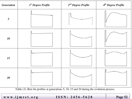
Table (2) shows the total number of fitness evaluations during the evolution process invoking the engineering simulation for each of the three fin profile shapes. In this case, the EA was run only once due to the time-consuming fitness. Table (3) shows the evolution of the shape of the fin profiles of the best individual in the population in each case with the number of generations.
Evolutionary Algorithm Parameters
Population size 100
Generations 20
Mutation Gaussian, probability=0.2 Crossover Two-point, probability=0.6
Selection Tournament, size=10
Elitism Yes, size=1
Table (1). Parameters of the evolutionary algorithm.
1st Degree 2nd Degree 4th degree
Number of Fitness
Evaluations 1479 1491 1493
Table (2). Number of fitness evaluations invoking heat-transfer simulator.
In the 1st, 2nd and 4th degree profile cases as the evolution proceeds, the base thickness (b) of the fin does not have a significant effect; itis seen to either decrease or remain constant, and is also closer to the minimum constraint in Equation (6). Since the vertical surfaces of the heat exchanger fin surrounded by air have not been considered in the fitness function in Equation (8), the profiles in Table (3) have low values for b. The same reason can be attributed to the high value of yav for the evolved fin profiles, since there is no implicit penalization in the EA for an individual with a high value of yav.
The higher values of yavrelative to the evolved values of s, manifests as a higher value of y0. This in turn decreases the variability in the remaining values of yi since there is an upper limit constraint on all the values of yi, the effect of which is more pronounced in the evolution of the 4th degree profiles.
However, with a small modification to the fitness function, high values of yavcan be mitigated which is addressed in section (4.3.2).
Generation 1st Degree Profile 2nd Degree Profile 4th Degree Profile
5
10
15
20
w w w . i j m r e t . o r g I S S N : 2 4 5 6 - 5 6 2 8
Page 53
As seen inTable (3) the curved surface of the fin profile evolvesto increase the surface area so that heat transfer to the fin tip can be enhanced. Also,in the case of the 4th degree profiles, the constraints incorporated tend to decrease the undulations on the curved surface of the fin. The evolution of the best and average fitness values over 20 generations for the linear, quadratic and 4th degree fin profiles are shown in Figure (5).
Figure (5) demonstrates that the 1st degree fin profile optimization attains a higher fitness value in 20 generations compared to the other shapes. This can be attributed to the smaller search space with a chromosome of length 4. In the evolution of the 1st degree profile, a high fitness individual is found early in the evolution process due to its smaller search space. Attaining a higher maximum fitness for the 2nd and 4th degree fin profiles is possible by changing the EA parameters like mutation, number of generations etc.
(a) 1st degree (b) 2nd degree
(c) 4th degree
Figure (5). Fitness evolution – EA based on engineering simulations.
Since the fitness function in Equation (8) does not account for the heat transfer from the vertical surfaces of the fin, modifying the fitness function can also improve the results of the EA. Each of these approaches requires additional time-consuming fitness evaluations.Thus, theapproach is not amenable to experimentation and restricts the quality of solutions obtained from the evolutionary optimization in higher dimensional search spaces. In the next section,the fitness function has been modified while utilizing the same parameters and constraints. The EA is run once again using a ROM and the Apache Spark based dataflow architecture and the results are discussed.
4.3.2. EA with Apache SparkbasedReduced Order Model
w w w . i j m r e t . o r g I S S N : 2 4 5 6 - 5 6 2 8
Page 54
(a) 1st degree (b) 2nd degree
(c) 4th degree
Figure (6). Fitness evolution - ROM based EA.
In Figure (6) it is seen that higher fitness values are obtained in all three cases by modifying the fitness function to include the transverse surface of the fin exposed to air. In the case of the 1st degree fin profile, the best chromosome in the population (maximum fitness) increases for 10 generations, after which the EA is unable to find a significantly better solution. This can be attributed to a smaller search space in the case of the 1st degree profiles. This is also reflected in the similarity of the fin profiles for generations 15 and 20 in Table (4).
Generation 1st Degree Profile 2nd Degree Profile 4th Degree Profile
5
10
15
20
w w w . i j m r e t . o r g I S S N : 2 4 5 6 - 5 6 2 8
Page 55
In the case of the 2nd degree profiles, higher fitness values are obtained throughout the evolution process. Also, in Figure (6) the 2nd degree fin profiles have evolved to maximize the surface area of the fin exposed to air which includes the transverse surface of the fin base. Similarly, in the case of the 4th degree profiles, the fitness of the best chromosome increasesthroughout the evolution process. The best chromosomes evolve to maximize the surface area of the fin, as well as evolve values of y0 and y4that allow for the most heat dissipation along the transverse surfaces of the fin. In each of the three cases, a higher fitness chromosome is obtained by updating the ROM with the elite chromosomes from each generation. The following section discusses the visualizations of the unified distance matrix plots from the SOM as well as an optimization case in which the constraints on the geometry have been modified.
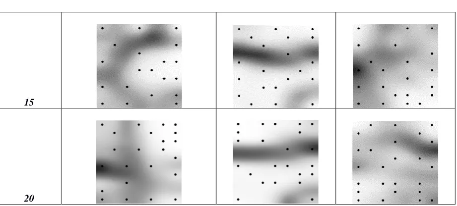
4.3.3. Discussion
In the approach taken in this article, elite chromosomes from the EA are utilized to update the ROM. To visualize changes to the input parameter space, a SOM unified distance matrix is used. Table (5) shows maps of the unified distance matrixat various stages of the evolution process. The unified distance matrix, which depicts distances between the input parameters, hasdarker regions implying greater distances at earlier generations and progressively moves towards being a more evenly spaced distribution.As the number of generations progresses the darker regions decrease. The EA adds additional points to the ROM input space, by
triggering engineering simulations which enhance the ROM. Additionally, it is also possible in the case of the 2nd degree profile, for the user to manually run simulations and update the ROM tobetter cover the input parameter space. The decrease in the space between data points in the input parameter space (i.e. darker regions), reflects better coverage of the input parameter space. This further underscores the role of the EA in enhancing the ROM. It can thus be concluded that visualizing using the SOM identifies regions of the input parameter space that need to be enhanced, in addition to the regions that are enhanced by the EA. Another example that underscores the usefulness of ROM based EAs is the ability to incorporate additional constraints on the fin geometry for improved manufacturability. Such design constraints are easier to incorporate quickly into a ROM based EA due to the lowcost of fitness evaluations. In the case of the 4th degree fin profile, the constraint on
y4is relaxed so it can assume any value in the range [0,1]. In addition, y2is constrained to be within a 20% range of y1. Figure (7) shows the evolution of fitness and geometries of the elite chromosomes at generations 5, 10, 15 and 20. It is seen that the fin profile at generation 20 evolves to one that is easier to manufacture despite having a lower fitness compared to the chromosome of the same generation in Table (4).
Thus, by utilizing Apache Spark as a data-store and to perform ROM computations at scale, it is possible to establish a data-flow loop where an EA can utilize the results of a ROM as well as update it with results from elite population at each generation.
Generation 1st Degree Profile 2nd Degree Profile 4th Degree Profile
5
w w w . i j m r e t . o r g I S S N : 2 4 5 6 - 5 6 2 8
Page 56
1520
Table (5). Visualization of unified distance matrix over generations.
Finally, the computational times are compared between the engineering simulation based optimization described in section 4.3.1 and the Spark - ROM based optimization described in section 4.3.2.
Figure (7). Evolution of fin profiles (generations 5, 10, 15,20)– modified constraints.
Fin profile Engineering Simulation EA Spark - ROM EA
1st degree 16 hrs. 3 hrs.
2nd degree 22 hrs. 3.2 hrs.
4th degree 23 hrs. 3.5 hrs.
Table (6). Run time comparison for 20 generations of the EA.
Since the Spark based ROM optimization involves bootstrapping 11 simulations, the time taken to run each of the initialsimulations has been included in the computational time. Also, since the ROM based optimization involves computing an engineering simulation and the SVD at the end of each
w w w . i j m r e t . o r g I S S N : 2 4 5 6 - 5 6 2 8
Page 57
both cases, the EA can be parallelized to further reduce the wall-clock computational time. However, the parallelization case has not been considered in this article and will in considered in future research. It is seen from Table (6) that the run time of the EA with the ROM is considerably less than invoking engineering simulations directly. The time variation across the fin profile degrees is explained by the additional time to run simulations as the complexity of the fin geometry increases. It must be noted that approximately 30% of the time for the Spark-ROM based EA is spent in running the simulations required for bootstrapping the ROM. It is thus seen that utilization of the proposed data-flow architecture can reduce the time required to optimize the shapes of heat-exchanger fins.
V. Conclusions and Future Work
This article demonstratesthe use of Apache Spark and the machine learning library MLlib for evolutionary optimization of an industrial system componenti.e. the shape optimization of a heat-exchanger fin. The article compares approaches invoking(a) high-fidelity engineering simulation models from an EA and (b)Spark-based ROMs from an EA.In the latter case, the best fitness chromosomes from each generation are used to augment the ROM, which results in higher performing optimal designs. SOMsare utilized to visualize the input design parameter space for the ROM and the visualizationsof the unified distance matrix are used to addsimulation data to assist the EA. Furthermore, constraints on the optimization problem are modified to adhere to manufacturability conditions and it is found that the ROM based EA can adapt and evolve a suitable solution. From theseresults, it can be concluded that through thisapproach the outcome of an EA utilizing ROMs can be directed and monitored in a transparent and efficient mannercompared to embedding a ROM into the EA. It also enables a more rapid exploration of the search space by utilizing data and machine learning driven reduced order models. Finally, the feedback of simulation data from the EAs elite solutionsenhances the ROM. This is a novel improvement from previous research where the results of the ROM were being employed by an optimization algorithm only to reduce computational time and not to re-compute the ROM on a periodic basis. Further researchneeds to be done toanalyze the performance by clustering Apache Spark nodes and analyzing performance on very large computational datasets. A detailed study and performance analysis can motivate further adoption of open-source big data tools by scientific computing researchers. Additionally, several open-source tools developed to process big data in real-time can be utilized to integrate engineering simulation models with real-time data from industrial systems equipment. Research needs to be
undertaken in this area to evaluate methods and architecturesfor connected industrial systemsto help enable the adoption of big data technologies in enterprises that utilize high-fidelity engineering simulation models todesign products.
References
[1.] Anflor, C. T. M., and R. J. Marczak.
"Topological sensitivity analysis for two-dimensional heat transfer problems using the Boundary Element Method." Optimization of Structures and Components. Springer International Publishing, 2013. 11-33.
[2.] Ashlock, Daniel. Evolutionary computation
for modeling and optimization. Springer Science & Business Media, 2006.
[3.] Cagnina, Leticia C., Susana C. Esquivel, and Carlos A. Coello Coello. "Solving engineering optimization problems with the simple constrained particle swarm optimizer." Informatica 32.3 (2008). [4.] Castellani, Michele, Yves Lemmens, and
Jonathan E. Cooper. "Parametric reduced order model approach for rapid dynamic loads prediction." Aerospace Science and Technology 52 (2016): 29-40.
[5.] Copiello, Diego, and Giampietro Fabbri.
"Multi-objective genetic optimization of the heat transfer from longitudinal wavy fins." International Journal of Heat and Mass Transfer 52.5-6 (2009): 1167-1176.
[6.] Deb, Kalyanmoy. Multi-objective
optimization using evolutionary algorithms. Vol. 16. John Wiley & Sons, 2001.
[7.] Dolci, V., and Renzo A. "Proper orthogonal decomposition as surrogate model for aerodynamic optimization." International Journal of Aerospace Engineering 2016 (2016).
[8.] François-Michel De R, Félix-Antoine F,
Marc-André Gardner, Marc Parizeau and
Christian Gagné, "DEAP -- Enabling
Nimbler Evolutions", SIGEVOlution, vol. 6, no 2, pp. 17-26, February 2014.
[9.] Fabbri, Giampietro. "Optimization of heat
transfer through finned dissipators cooled by laminar flow." International Journal of Heat and Fluid Flow 19.6 (1998): 644-654. [10.] Gunzburger, M.D. Perspectives in flow
control and optimization. Society for industrial and applied mathematics, 2002. [11.] Holland, J. Adaptation in natural and
artificial systems: an introductory analysis with applications to biology, control, and artificial intelligence. MIT press, 1992. [12.] Incropera, F.P. and De Witt, D.P.,
Fundamentals of Heat and Mass Transfer, 4th edition, John Wiley, New York, 2002. [13.] Jansen, Jan Dirk, and Louis J. Durlofsky.
w w w . i j m r e t . o r g I S S N : 2 4 5 6 - 5 6 2 8
Page 58
control optimization." Optimization and Engineering 18.1 (2017): 105-132.
[14.] John, Anish K., and K. Krishnakumar. "Performing multiobjective optimization on perforated plate matrix heat exchanger surfaces using genetic algorithm." International Journal for Simulation and Multidisciplinary Design Optimization 8 (2017): A3.
[15.] Kaveh, A., and A. Dadras. "A novel meta-heuristic optimization algorithm: Thermal exchange optimization." Advances in Engineering Software (2017).
[16.] Kirby, Michael. Geometric data analysis: an empirical approach to dimensionality reduction and the study of patterns. John Wiley & Sons, Inc., 2000.
[17.] Liu, W., Zhang, T., Xue, Y., Zhai, Z. J.,
Wang, J., Wei, Y., and Chen, Q. (2015).
State-of-the-art methods for inverse design of an enclosed environment. Building and Environment, 91, 91-100.
[18.] Lohan, Danny J., Ercan M. Dede, and James T. Allison. "Topology optimization for heat conduction using generative design algorithms." Structural and Multidisciplinary Optimization 55.3 (2017): 1063-1077.
[19.] Ly, H. V., and Tran, H. T. (2001). Modeling and control of physical processes using proper orthogonal decomposition. Mathematical and computer modelling, 33(1-3), 223-236.
[20.] Magstadt, A. S., Kan, P., Berger, Z. P., Ruscher, C. J., Berry, M. G., Green, M. A., and Glauser, M. N. (2017). Turbulent flow physics and control: The role of big data analyses tools. In Whither Turbulence and Big Data in the 21st Century? (pp. 295-322). Springer International Publishing.
[21.] Meng, Xiangrui, et al. "MLlib: Machine learning in apache spark." The Journal of Machine Learning Research 17.1 (2016): 1235-1241.
[22.] Özisik, Necati M., Finite Difference Methods in Heat Transfer, CRC Press, Boca Raton, 1994.
[23.] Peremezhney, Nicolai, et al. "Combining Gaussian processes, mutual information and a genetic algorithm for multi-target optimization of expensive-to-evaluate functions." Engineering Optimization 46.11 (2014): 1593-1607.
[24.] Ritter, Helge, et al. Neural computation and self-organizing maps: an introduction. Reading, MA: Addison-Wesley, 1992. [25.] Reddy, P. Swapna, K. Yamuna Rani, and
Sachin C. Patwardhan. "Multi-objective optimization of a reactive batch distillation process using reduced order
model." Computers & Chemical Engineering (2017).
[26.] Stefanovic, Pavel, and Olga Kurasova.
"Visual analysis of self-organizing maps." Nonlinear Analysis: Modelling and Control 16.4 (2011): 488-504.
[27.] Steinbach, M., Karypis, G., & Kumar, V.
(2000, August). A comparison of document clustering techniques. In KDD workshop on text mining (Vol. 400, No. 1, pp. 525-526). [28.] Suram, S., K. M. Bryden, and D. A. Ashlock.
"An evolutionary algorithm to estimate unknown heat flux in a one-dimensional inverse heat conduction problem." Proceedings of the 5th International Conference on Inverse Problems in Engineering: Theory and Practice. Vol. 11. 2005.
[29.] Suram, S, Ashlock, D.A, and Bryden, K.M.
"Graph based evolutionary algorithms for heat exchanger fin shape optimization." American Institute of Aeronautics and Astronautics Inc., Portsmouth, VA, United States (2006): 647-657.
[30.] Suram, S., McCorkle, D., and Bryden, K.M.,
“Proper Orthogonal Decomposition-Based Reduced Order Model of a Hydraulic Mixing Nozzle." AIAA MAO, Vancouver, Canada (2008).
[31.] Ullman, David. The mechanical design
process. McGraw-Hill
Science/Engineering/Math, 2009.
[32.] Ushijima, Timothy T., and William WG Yeh.
"Experimental design for estimating unknown hydraulic conductivity in an aquifer using a genetic algorithm and reduced order model." Advances in Water Resources 86 (2015): 193-208.
[33.] Xiao, D., Fang, F., Pain, C. C., Navon, I. M., Salinas, P., and Muggeridge, A. (2015). Non-intrusive reduced order modeling of multi-phase flow in porous media using the POD-RBF method. submitted to Journal of Computational Physics.
[34.] Xu, W, et al. "Improving evolutionary algorithm performance for integer type multi-objective building system design optimization." Energy and Buildings 127 (2016): 714-729.
[35.] Yepes, V., J. V. Martí, and T. García-Segura. "Design optimization of precast-prestressed concrete road bridges with steel fiber-reinforcement by a hybrid evolutionary algorithm." International Journal of Computational Methods and Experimental Measurements 5.2 (2017): 179-189.