Blocking Optimization Techniques for Sparse Tensor Computation
Jee W. Choi
IBM T. J. Watson Research Center Yorktown Heights, NY, USA
Xing Liu∗
Parallel Computing Laboratory Intel Corporation Santa Clara, CA, USA [email protected]
Shaden Smith University of Minnesota Minneapolis, MN, USA
Tyler Simon University of Maryland,
Baltimore County Baltimore, MD, USA [email protected]
Abstract—We present a detailed analysis of the sparse matricized tensor times Khatri-Rao product (MTTKRP) kernel that is the key bottleneck in various sparse tensor computations. By using the well-known roofline model and carefully instru-menting the state-of-the-art MTTKRP code with the pressure point analysis technique, we show that the performance of MTTKRP is highly sensitive to data traffic like other sparse computations. We also identify key performance bottlenecks that diverge from our prior knowledge of sparse MTTKRP on modern processors.
We propose to use blocking optimization techniques to address the bottlenecks identified within the MTTKRP com-putation. By using a combination of two blocking techniques, we achieve more than 3.5× and 2.0× speedup over the state-of-the-art MTTKRP implementation in the SPLATT library on four real-world data sets and two synthetically generated data sets, respectively. We also employ a new data partitioning technique for the distributed MTTKRP implementation, which provides an additional dimension of scalability. As a result, our implementation exhibits good strong scaling and a 1.6×
speedup on 64 nodes for two real-world data sets, when compared to the SPLATT library.
Keywords-tensor, decomposition, canonical polyadic, MPI, distributed, high-performance computing, MTTKRP
I. INTRODUCTION
We conduct a low-level performance analysis and blocking optimization of the sparse matricized tensor times Khatri-Rao product (MTTKRP) - a key computational bottleneck in various sparse tensor computations. Sparse tensor com-putations - in particular, tensor decompositions such as the canonical polyadic decomposition (CPD) - are becoming increasingly popular in the HPC community for analyzing large quantities of data with multi-dimensional relationships. Therefore, having anefficientandscalable implementation of sparse MTTKRP is highly desirable for a wide variety of applications. Signal processing, computer vision, network intrusion detection, and machine learning [1], [2] are just a few of the many fields that employ tensor computations.
Our study shows that sparse MTTKRP operations are memory bound even for extremely high ranks; therefore, op-timization strategies should focus on minimizing data move-ment from slow memory. This is in contrast to what many other researches have been focusing on, which is minimizing the total number of floating point operations [3]–[5]. In this paper, we employ blocking optimization techniques to address performance bottlenecks of sparse MTTKRP, identified from a careful performance analysis. While reducing computation
∗During the period of this research, Xing Liu was affiliated with IBM T.
J. Watson Research Center.
may alsoindirectlyreduce data movement, our work explicitly targets opportunities for reducing data movement through various blocking techniques.
Even though blocking techniques have been well studied in other sparse computation methods such as sparse matrix-vector multiplication [6] (SpMV) and sparse matrix-matrix multiplication [7] (SpGEMM), a systematic study on applying blocking techniques to tensors has not yet been conducted. Also, due to the inherent complexity of high-order compu-tation, experience from prior work in other fields can not easily be applied to tensors. This was demonstrated in the work by Smith et al. [4], where re-ordering nonzeros through hypergraph partitioning yielded very little improvement in performance. We do, however, leverage their work to conduct a more systematic analysis of the interaction between various properties of a tensor and how they influence memory access.
Findings and contributions: This paper makes three key contributions to the understanding and performance of sparse MTTKRP.
1) Analysis: Using the roofline model and the pressure point analysis (PPA) technique, we systematically ana-lyze and identify key bottlenecks in the state-of-the-art MTTKRP kernel from the SPLATT library [4]. We show that there are two key bottlenecks in the SPLATT MTTKRP kernel - pressure on the load units in the micro-architcture, and main memory access to the factor matrices (Section IV). We also highlight notable performance trends in our results and correlate them to properties of the tensor. (Section VI)
2) Optimization:After identifying targets for optimization, we selectively apply a series of blocking techniques to the baseline SPLATT implementation to improve its performance, including a novel blocking method that is specific to tensor computation. We achieve up to 2.0× speedup over baseline SPLATT MTTKRP for two synthetically generated data sets with Poisson distribution, and an even higher 3.5×speedup for four real-world data sets on a single IBM POWER8 processor. (Section V, VI)
partitioning scheme adopted by SPLATT on a cluster of 64 IBM POWER8 nodes.
To the best of our knowledge, our work is the first to systematicallystudy the performance bottlenecks of sparse MTTKRP and explore the use of various blocking techniques to improve its performance on both shared memory and distributed systems. Beyond the analysis and the performance improvements, our work demonstrates the importance of exploiting structure within real-world data, and paves way for new avenues of research in performance modeling and auto-tuning sparse tensor decomposition.
II. RELATEDWORK
Due to the rise of big data analytics, tensors have become popular in the HPC community. A significant amount of recent work has focused on optimizing tensor computations in sequential, shared memory parallel, and distributed settings.
The MATLAB Tensor Toolbox [10] is a widely-used tensor package, which provides a sequential implementaion for both dense and sparse tensors. Tensorlab provides another sequential MATLAB implementation, which can be used to rapidly prototype various tensor decomposition methods with structured factors.
The work by Li et al. [11] focuses on shared memory optimizations for dense tensors, in which they propose in-place computation for the tensor-times-matrix multiply that dramatically reduces data movement. The most recent work on sparse tensor computations are SPLATT [4] and its higher order generalization – CSF, by Smith et al. [12]. They are also among the fastest tensor implementations and are used in this paper as the performance baseline. SPLATT was also optimized for the Intel Xeon Phi Knights Landing architecture which features both DDR4 and MCRDAM (high-bandwidth) memory [13]. SPLATT allocates its factor matrices in MCDRAM and the tensor data itself in the larger DDR4 memory.
In the category of distributed parallel implemtations, Cyclops Tensor Framework [14] uses OpenMP+MPI par-allelism and focuses on communication reduction for tensor contraction. GigaTensor [3] is a tensor implementation that uses the MapReduce framework, and it restructures MTTKRP as a series of Hadamard products. Many work on distributed tensor algorithms focus on data distribution. DFacTo [5] and SALS [15] use coarse-grained distribution, in which only one tensor mode is partitioned across MPI processes and each process own a set of contiguous slices of the tensor. In contrast, the work by Smith et al. [8] uses the medium-grained decomposition, in which all tensor modes are partitioned. HyperTensor [16] uses the fine-grained decomposition to partition nonzeros individually. More recently, HyperTensor was extended to include memoization, which trades off storage overhead in order to reduce the cost of individual MTTKRP operations [17].
III. TENSOROVERVIEW
We begin by providing a brief overview of MTTKRP and related tensor notations. For a more in-depth discussion of tensors and tensor computations, including their applications, we direct the readers to several extensive surveys [1], [2].
A. Notations
Tensors are the higher-order generalization of matrices. An N dimensional tensor ia also referred to as havingN modes (a mode-N tensor) or anorder N. The following notations are used in this paper:
1) Scalarsare denoted by lower case letters (e.g., a). 2) Vectors are mode-1 tensors and are denoted by bold
lower case letters (e.g.,a). Theith element of a vector
a is denoted byai.
3) Matrices are mode-2 tensors and are denoted by bold capital letters (e.g., A). If A is aI×J matrix, it can also be denoted as A∈RI×J, and its element(i,j)is
denoted as ai,j.
4) Higher-order tensors are denoted by Euler script letters (e.g.,
X
). A mode-N tensor whose dimensions areI1× I2× · · · ×IN can be denoted asX
∈RI1×I2×···×IN, andits element(i1,i2, . . . ,iN)is denoted asxi1,i2,...,iN.
5) Fibers are the higher-order analogue of matrix rows and columns. A mode-nfiber is defined by fixing every mode except thenth mode.
B. MTTKRP
MTTKRP is a common kernel in many tensor applications and the most expensive part of tensor decompositions [4]. It consists of two basic tensor operations: thetensor matriciza-tionand theKhatri-Rao product.
1) Tensor matricization is the process of flattening or unfolding a tensor into a matrix. This operation is best understood as the rearrangement of fibers as columns of a matrix. That is, in the mode-nmatricization of a tensor
X
, denoted by X(n), the mode-n fibers ofX
are laid out as columns of X(n). For a tensorX
∈RI1×I2×···×IN,X(n) is a matrix of sizeIn×Iˆn, where ˆIn=∏i6=nIi.
2) Khatrio-Rao product is the “matching column-wise” Kronecker product between two matrices. That is, given two matrices B ∈ RJ×R andC ∈RK×R, their
Khatri-Rao product K, denoted byK=BC, whereKis a
(J·K)×Rmatrix, is defined as
BC= [b1⊗c1b2⊗c2. . .bR⊗cR]
Although we cover this operation for understanding purposes, it is not usually formed explicitly in sparse MTTKRP implementations, as we will see in the next section.
In the context of tensor decompositions, for a mode-3 tensor
X
∈RI×J×K, the mode-1 MTTKRP can be expressedas A=X(1)(BC). Here, A ∈ RI×R, B ∈ RJ×R, C ∈ RK×R are called the mode-1, mode-2 and mode-3 factor
i index j index k index val
1 1 1 5
1 2 2 3
1 2 3 1
2 1 3 2
2 2 2 9
2 3 3 7
3 1 1 9
(a)Coordinate format
0
3 5
5
3
1
9 2 7 9 1
2
2
2 1 3 1 j_index val
0
1
2
3 4 6
i_pointer k_pointer
1
2
3
2 3 1 k_index
row 1 row 2
row 3
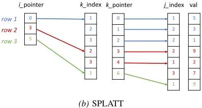
(b)SPLATT
Figure 1:Sparse tensor formats for a 3×3×3 tensor
C. Sparse MTTKRP
In MTTKRP, the Khatrio-Rao productBCis a dense
(J·K)×R matrix. Computing and storing BC for any moderate sized tensor is prohibitively expensive. An efficient MTTKRP algorithm usually does not formBCexplicitly, and how it is calculated depends on the sparse data structures used to store the tensor, which we will describe below.
Sparse tensors are stored in a manner similar to sparse matrices. The two most commonly used data structures are the coordinate (COO) format [18], where each nonzero value is stored with its coordinates, and the 3D analogue to the compressed sparse row (CSR) format, the SPLATT format [4]. The higher-order extension to SPLATT is the compressed sparse fiber (CSF) [12] format. However, in this paper, we focus our optimization efforts on the SPLATT format and 3D data, as it simplifies profiling and analysis, but our methodology and result can trivially be extended to higher-order data.
1) COO Format: Figure 1a shows a 3×3×3 tensor in the COO format, where each nonzero (stored in val) is coupled with its (i,j,k)coordinates (stored in i index, j indexand k index). The main advantage of this format is that the coordinates of any nonzero element can be accessed easily. As an example, we now describe the mode-1 MTTKRP kernel for a sparse tensor
X
∈RI×J×Kin the COO formatand for rank R. For each nonzerot with coordinates(i,j,k)
and valuev, we compute the Khatri-Rao producton the fly by fetching the jth andkth rows ofBandC, and computing the Hadamard product between the two length-Rvectors. We then scale the vector by v. This computes the nonzerot’s contribution to theith row ofA, and this is repeated until allnnznonzeros have been processed.
2) SPLATT Format: Figure 1b presents the SPLATT format for the same tensor shown in Figure 1a. SPLATT stores nonzeros in groups of fibers (mode-2 fibers). For each row i, the i pointer structure points to the first and the lastnon-empty fiber in its row, tracked by thek indexand k pointer structures.k index stores the mode-3 index of the fiber (only onek indexvalue is needed for all nonzeros in a fiber), andk pointerpoints to the first and the last nonzero in its fiber. The structuresvalandj indextracks the nonzero values and the mode-2 index of each nonzero, respectively. For a mode-3 tensor with nnznonzeros, the amount of memory required to store tensors in the COO format is 32×nnzbytes (using 64-bit for index and double precision for value). For the SPLATT format, if the same tensor has F non-empty fibers, then the amount of memory required to
store it is 16×F+16×nnzbytes.
Using the SPLATT format provides two key advantages over using the COO format. First is the reduction in the data structure size, and second is the reduction in computation and data movement that comes as a result of the CSR-like nature of the storage format. Algorithm 1 shows the SPLATT implementation taken straight from the source code1(it has been slightly edited and uses variable names from Figure 1b to make it more readable).
Algorithm 1 SPLATT MTTKRP algorithm for a sparse tensor
X
∈RI×J×Kand rankR1: A←0
2: fori←0 toI do
3: for j←i pointer[i]toi pointer[i+1]do
4: s←0
5: fork← k pointer[j]tok pointer[j+1]do
6: forr←0 toRdo
7: s[r] + =val[k]×B[j index[k]] [r]
8: forr←0 toRdo
9: A[i] [r] + =s[r]×C[k index[j]] [r] 10: returnA
As seen in Algorithm 1, instead of multiplying each nonzero value by rows from bothB and C before adding to A, the SPLATT MTTKRP algorithm first multiplies each nonzero value to a row from B(line 6–7), and then accumulates this intermediate result forallnonzeros in the fiber before finally multiplying (via Hadamard product) it to the row fromC(line 9–10). Therefore, more nonzeros there are in the fiber, more computation and data movement that can be saved.
While it is clear how many floating point operations can be saved over COO using SPLATT, the amount of data movement from memory that can be saved is unclear, due to the complex nature of the interaction between the code and the underlying hardware architecture (e.g., cache size and hierarchy, replacement policy, etc.)
To the best of our knowledge, SPLATT is the fastest available shared memory implementation of MTTKRP [9], [12] and is widely used in shared and distributed MTTKRP implementations [19]. Therefore, we focus our study on the SPLATT MTTKRP algorithm.
IV. IDENTIFYINGBOTTLENECKS INMTTKRP In this section, we identify potential bottlenecks in the SPLATT MTTKRP kernel using the well-known roofline
model [20] and the pressure point analysis (PPA) method [21]. A. Roofline model analysis
0.1 1 10 100 1000
16 32 64 128 256 512 1024 2048
Ari
thme
tic
In
tensity
Rank
α = 1.0 α = 0.95 α = 0.9 α = 0.8 α = 0.7 α = 0.6 α = 0.4 α = 0.2 α = 0.0
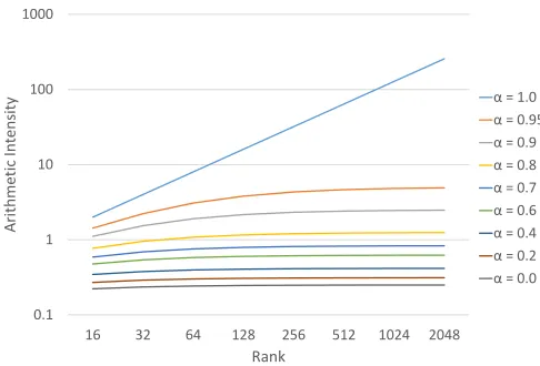
Figure 2:Arithmetic intensity of SPLATT MTTKRP for different cache hit rates and rank sizes
We start by analyzing the baseline SPLATT kernel de-scribed in Algorithm 1 using the roofline model. The roofline model is a visually-intuitive and throughput-oriented method for representing a system’s performance characteristics [20]. Itplotsa system’s performance for various arithmetic inten-sities(floating–point operations per byte of DRAM traffic) of algorithms. This visualization and mapping of performance to algorithm helps to quantify the primary factors that are limiting the performance of a given application.
Equations 1-3 approximate the amount of data required from memory (Q), the number of floating point operations (W), and the arithmetic intensity (I) of SPLATT MTTKRP, in whichnnzis the number of nonzeros,F is the number of non-empty fibers,R is the rank, andαis the overall cache hit rate (which depends on both the sparsity pattern of the tensor and the underlying hardware), and all data types (for both values and indices) are assumed to be 64-bits long.
In terms of data structures (Figure 1b), the first term in Equation 1 (2nnz) accounts for access to val and j index, the second term (2F) accounts for access to k index and k pointer, the third term ((1−α)·R·nnz) accounts for access to the mode-2 factor, and the fourth term ((1−α)·R·F) accounts for access to the mode-3 factor. We ignore access to i pointer since its size is negligible in comparison to the rest, and we also ignore access to the mode-1 factor (destination factor), since its re-use distance is short and therefore likely to be always in the cache.
Q = 2nnz+2F+
(1−α)·R·nnz+ (1−α)·R·F (1)
W = 2R(nnz+F) (2)
I = W
Q·8bytes=
R
8+4R(1−α) (3) From Equation 3 we can derive that the arithmetic intensity of SPLATT MTTKRP ranges from R/(8+4R)whenα=0 to R/8 when α=1. Since we do not know exactly what the cache hit rate would be without knowing the data and
the system architecture, we show how arithmetic intensity changes with respect to rankRfor theentire rangeof possible cache hit rates in Figure 2 . Even for a very high cache hit rate of 95%, the arithmetic intensity ranges from 1.43 at rank 16 to at most 4.90 at rank 2048. Given that state-of-the-art CPUs and GPUs today have system balance ranging from 6 to 12, SPLATT MTTKRP will likely be memory bound in most cases. Only when the data fits completely in the cache andthe rank is high enough (>64), can SPLATT MTTKRP become compute bound.
Moreover, the equation suggests that the largest portion of that data will come from the mode-2 factor matrix (i.e.,
(1−α)·R·nnzfrom Equation 1), asnnzis typically much larger thanF. The fact that one particular factor matrix is the primary contributor to memory traffic is a little surprising and diverges from our intuitions, since a factor matrix is much smaller than the the tensor.
B. Pressure point analysis
In order to validate our conclusion that SPLATT MTTKRP is memory bound and to isolatespecificsections of the code that create bottlenecks, we perform a variation of the pressure point analysis (PPA) [21] on the SPLATT MTTKRP kernel. The idea behind PPA is to create artificial “pressure points” in the code (e.g., insert/delete instructions to affect utilization, altering memory access addresses to change the cache hit rate, or renaming registers to change dependencies) to gain a better understanding ofwhich resourcesin the micro-architecture are causing performance to change, andwhere in the code this is happening.
Table I shows five pressure points of interest in the SPLATT MTTKRP kernel running on a 30K×30K×30K sparse tensor with 135 million nonzeros. The tensor is synthetically generated with Poisson distribution, and the execution time was measured on a IBM POWER8 server. We limited the execution to a single core to negate non-uniform memory access (NUMA) effects, while using two hardware threads to maximize performance.
The type 5 pressure point moves the per-fiber floating-point operations (line 8-9 in Algorithm 1) to the per-nonzero inner-loop (line 5 in Algorithm 1) to “emulate” the COO kernel. This increases floating point operations but has minimal impact on the execution time (1.54%), suggesting that computation is not a bottleneck for SPLATT MTTKRP.
Table I:Pressure points for SPLATT MTTKRP
Type Exec. Time Description
1 1.63 Access toBremoved
2 1.81 All accesses toBis limited to L1 3 2.11 Eliminating load instructions
4 2.43 Access toCremoved
5 2.64 Moving flops to the inner-loop
6 2.60 Unchanged
matrix is much more expensive than accessing the mode-3 factor matrix and is actually the most expensive component of SPLATT MTTKRP. In addition, instead of eliminating access completely, if we change the pattern of access toBso that every access is limited to the first row of the matrix (and therefore accessed exclusively from the L1 cache), then we reduce the execution time by30.32%(type 2). This indicates that caching the factor matrixBshould improve performance significantly.
Lastly, eliminating the load instructions (type 3) to the accumulator (line 7 and 9 from Algorithm 1) reduces the execution time by18.77%. Since the accumulator is small in size (8R bytes per thread) and frequently accessed, it likely resides in the L1 cache. Therefore, we can reasonably assume that this improvement comesnot from eliminating access to the main memory, but from reducing the pressure on the load units in the pipeline.
From our analysis, we can draw three key conclusions. 1) SPLATT MTTKRP is highly memory bandwidth limited
unless all the factor matrices are small enough to completely fit into the cache and the rankR is large enough (>64). Therefore we should focus on reducing memory traffic, rather than reducing flops.
2) Accessing the mode-2 factor matrix B is the most expensive component – more expensive than access-ing/streaming the tensor. We should attempt to maximize cache re-use for this factor matrix.
3) There exists a load unit pressure in the SPLATT MTTKRP kernel, whose cost is comparable to accessing the mode-2 factor matrix. It mainly comes from the innermost loop where the MTTKRP kernel accesses the mode-2 factor matrix and the accumulator array. To improve the performance of SPLATT MTTKRP, we should also attempt to address this bottleneck.
V. BLOCKINGTECHNIQUES
In Section IV, we discovered that the load unit pressure due to accessing the accumulator array and reading the mode-2 factor matrix from memory are the two major bottlenecks in SPLATT MTTKRP. In this section, we propose to use a combination of two blocking techniques to address these two bottlenecks.
While blocking is commonly used to improve the perfor-mance of various sparse matrix kernels, e.g., sparse matrix-vector multiply, how to apply it to tensor computation is not obvious and relatively more difficult, mainly due to the inherently complex nature of high order sparse computations. Existing research has used re-ordering techniques to improve the data locality of MTTKRP, which requires expensive graph partitioning and extensive reorganization of the original data structure, but observed only a small improvement in performance [4]. In contrast, the blocking optimization techniques presented in this section require very little data rearrangement and overhead.
A. Multi-dimensional blocking
The most obvious way to employ blocking techniques for tensors is to block the data along modes - similarly to how data is blocked in sparse matrix-vector multiply - in an
attempt to fitrows of factor matrices into the cache. This is intuitive since a row of the factor matrix represents the granularity of computation - ı.e., each nonzero scales a row of the factor matrices. Figure 3a shows an example of blocking for a mode-3 tensor, where the tensor has been blocked into 2×3×2 blocks. In order to process the sub-tensor
X
1, you would require contributions from the sub-matricesA1, B1, andC1. If the sub-matrices are small enough, then the rows would be accessed mostly from the cache, rather than being streamed from the slow memory every time it is needed. We call this blocking mechanismmulti-dimensional blocking (MB).The downside of multi-dimensional blocking is that the number of redundant accesses to the factor matrices are increased overall. That is, if the tensor has been blocked into NA,NB, andNC blocks along mode-1, mode-2, and mode-3,
respectively, then the number of times each factor matrix has to be accessed is as follows:
1) A(mode-1):NB×NC times
2) B (mode-2):NA×NC times
3) C(mode-3):NA×NB times
The goal of multi-dimensional blocking is to increase the cache hit rate enough so that the penalty of redundant access to the slow memory can be amortized by accessing as much of the data as possible from the cache. Therefore, it is also entirely possible to end up with lower performance by loading more data from the slow memory if non-optimal blocking sizes are used. Finding the optimal blocking size for every mode is prohibitively expensive for very high order tensors. We will discuss how to select the optimal blocking sizes in Section V-C
Additionally, to implement multi-dimensional blocking, we need to reorganize the tensor data so that the nonzeros in each block are stored continuously. However, this cost is negligible compared to the reordering methods, such as the graph partitioning used in [4], and can be amortized by the 10-1000s of iterations of the CPD algorithm.
B. Rank blocking
We propose a new type of blocking that is specific to tensor decomposition -rank blocking(RankB). Rank blocking divides factor matrices along the rank (or columns) into
NRankB strips with a size ofI×BSRankB, where BSRankB=
R/NRankB. Contribution to the ith strip of the mode-3 factor
matrixCcan be computed independently of other strips and only requires accessing theith strip ofAandB. Algorithm 2 illustrates the MTTKRP implementation using rank blocking.
Since granularity of computation for MTTKRP is by row, blocking along the rows may seem more intuitive. However, since we have determined that sparse MTTKRP is memory bound, it is more important to consider the granularity of memory access. Blocking along the rank of a factor matrix will allow more rows to fit in cache, thereby increasing the chance of finding a particular row in cache.
X1 A1
B1
C1
(a)Multi-dimensional (2×3×2) blocking
X1 A1
B1
C1 BSRankB
BSRankB BSRankB
(b)Combining multi-dimensional blocking with rank blocking (2×
3×2×NRankB)
Figure 3:Blocking of a tensor
Algorithm 2 MTTKRP algorithm with rank blocking for a sparse tensor
X
∈RI×J×K(rank =R andNRegB=16).1: A←0 2: rr←0 3: ip←i pointer 4: k p←k pointer 5: ki←k index 6: ji←j index 7: whilerr<Rdo 8: fori←0 toI do
9: for j←ip[i]toip[i+1]do 10: forr←rrtorr+BSRankB do
11: reg0←0
12: . . .
13: reg15←0
14: fork←k p[j]tok p[j+1]do
15: reg0 +=val[k]×B[j index[k]] [r+0]
16: . . .
17: reg15 +=val[k]×B[ji[k]] [r+15] 18: A[i] [r+0]+=reg0×C[ki[j]] [r+0]
19: . . .
20: A[i] [r+15]+=reg15×C[ki[j]] [r+15]
21: r+= 16
22: rr+=BSRankB 23: returnA
the cache hit rate may not increase significantly through multi-dimensional blocking alone. Figure 3b shows an example that combines multi-dimensional blocking with rank blocking.
Applying rank blocking allows us to use the register blocking technique to reduce the load unit pressure caused by accessing the accumulator array. Algorithm 2 also shows how to apply the register blocking technique with rank blocking. In Algorithm 1, lines 6–7 multiply each nonzero in a fiber with a row from matrixBand accumulates the result, which requires loading the entire accumulator array once per nonzero. We can divide the accumulator array into NRegB blocks, and
process the fiber inNRegBsteps. At each step, the nonzeros
in the fiber are multiplied with the entries from only one block of the accumulator array. If each block of the accumulator array is small enough to fit into registers, it can completely eliminate the use of the accumulator array, which reduces the number of load instructions.
Note that while the nonzeros in each fiber are accessed redundantlyNRegBtimes, they are always found in the cache
due to their extremely short re-use distance. The size of register blocking is limited by the number of available
hardware registers and should be chosen as a multiple of the cache line size.
Lastly, rank blocking can be used in a distributed setting to improve scalability. The medium-grained decomposition used by SPLATT [8] suffers from load imbalance and high communication overhead issues on a large number nodes (see Section VI-D for details on the medium-grained decomposition). By first partitioning the processor along the rank, and then partitioning each subset of processors using the medium-grained decomposition, the number of nonzeros assigned to each processor will be larger than the medium-grained decomposition, without increasing the communication complexity, since operations on different blocks along the rank are completely independent. For example, in Figure 3b, the processors can been divided into a 2×3×2×NRank grid, whereNRank=2. Therefore, there
will be two copies of the tensor
X
among the processors, one copy for each 2×3×2 set, and each set will work on separate, non-overlapping blocks along the rank.While not necessary, a small rearrangement of the factor matrix can allow rank blocking to work more efficiently. The tall and narrow strips of the factor matrix are stacked on top of each other to make(I·NRank)×BSRank matrix. This
is done to ensure a more sequential access to the memory, which, in turn, allows the hardware prefetcher to work more efficiently, as well as to reduce the number of expensive page misses.
C. Selecting the blocking sizes
Table II:Synthetic and real world data sets used for our experiments
Name Dimensions NNZ Sparsity
Poisson1 256×256×256 1.5M 8.8e-2 Poisson2 2K×16K×2K 121M 1.9e-3 Poisson3 30K×30K×30K 135M 5.0e-6 NELL2 12K×9K×29K 77M 2.4e-5 Net f lix 480K×18K×80 80M 1.2e-4 Reddit 1.2M×23K×1.3M 924M 2.8e-8 Amazon 4.8M×1.8M×1.8M 1.7B 2.5e-8
factor matrix is the least expensive. The cost of this heuristic is
O
(log2In), where In is the length of the mode, and isrelatively inexpensive compared to the 10-1000s of iterations required for decomposition.
VI. EXPERIMENTALRESULT ANDANALYSIS We present our experimental result and analysis for various real and synthetic data sets.
A. Test platform and data sets
1) Test platform: We evaluate our implementations on a distributed system of IBM POWER8 processor. Each node of the system is equipped with two POWER8 processors, and each processor consists of 10 8-way SMT cores, with 64KB and 512KB of L1 and L2 cache per core. Each core runs at a maximum of 3.49 GHz, and is capable of issuing two independent 128-bit SIMD FMA instructions per cycle. The memory bandwidth of each node is approximately 150 GB/s for read and 75 GB/s for write.
2) Data sets: The synthetic and real world data sets that we use for evaluation are presented in Table II. Poisson1-Poisson3 are synthetically generated data with Poisson distribution. We use data with Poisson distribution (or “count” data), as such data is found in a wide range of real applications, ranging from network traffic monitoring [22] to social networks [23]. Tensor decomposition of Poisson data was explored in prior work by Hansen et al. [24] and Chi et al. [25], and we use the same method presented in those papers to generate our Poisson data.
Netflix [26], NELL2 [27], Amazon [28], and Reddit [29] are real world data sets that are commonly used in tensor decomposition research for evaluation purposes [4], [15], [16].
3) Execution environment: We use SPLATT v1.1.1 as the baseline for all our comparisons. In order to do a fair compar-ison, we added our implementation directly to the SPLATT source code. Unless otherwise noted, every single-processor evaluation was done using 10 cores (one socket), with two threads per core. Speedups are measured by comparing the execution times for the mode-1 MTTKRP, average over 20 runs. For evaluating the distributed implementation, we use both sockets by assigning one MPI rank per socket, for a total of two MPI ranks per node.
B. Impact of blocking sizes on performance
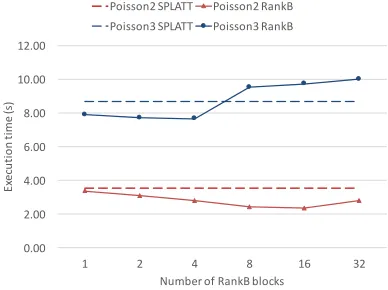
Figure 4 shows how the performance changes with respect to the number of blocks along the rank for Poisson2 and Poisson3 for a rank of 512. For Poisson2, rank blocking
0.00 2.00 4.00 6.00 8.00 10.00 12.00
1 2 4 8 16 32
Ex
ec
ut
io
n
tim
e
(s
)
Number of RankB blocks Poisson2 SPLATT Poisson2 RankB Poisson3 SPLATT Poisson3 RankB
Figure 4:Performance vs. RankB blocking size
always yields better performance; however, there is distinct “sweet spot” when 16 blocks are used. The result ofPoisson3 shows that the performance can beworseif the block sizes are chosen poorly.Poisson3 achieves the best performance with 4 rank blocks. The performance drops to below that of the baseline SPLATT implementation and becomes progressively worse with larger number of blocks.
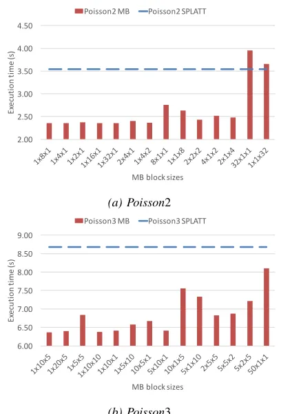
Figure 5 shows how the performance changes with respect to the number of blocks along the modes. For Poisson2 (shown in Figure 5a), due to the extremely long mode-2 lengths, blocking along this mode alone yields good perfor-mance, but the actual number of blocks has little impact (first five left columns in red). Additionally blocking along mode-1 (e.g., mode-1×4×1 vs. 2×4×1) or mode-3 generally degrades performance, and blocking along mode-3 is generally better than blocking along mode-1 (e.g., 8×1×1 vs. 1×1×8), which is expected, since mode-3 is accessed much more frequently. In extreme cases (the two right-most columns), the performance could be worse. ForPoisson3, as shown in Figure 5b, every blocking size yielded better performance than the baseline SPLATT implementation. Again, blocking along mode-3 is generally better than blocking along mode-1, and the best performance is observed when the block sizes are 1×10×5.
The results demonstrate that our heuristic can find blocking sizes for both the MB and RankB blocking methods that lead at the very least to local execution time minima. C. Single processor results
2.00 2.50 3.00 3.50 4.00 4.50
Ex
ec
ut
io
n
tim
e
(s
)
MB block sizes Poisson2 MB Poisson2 SPLATT
(a) Poisson2
6.00 6.50 7.00 7.50 8.00 8.50 9.00
Ex
ec
ut
io
n
tim
e
(s
)
MB block sizes Poisson3 MB Poisson3 SPLATT
(b) Poisson3
Figure 5:Performance vs. MB blocking size: the left most block sizes give the best performance.
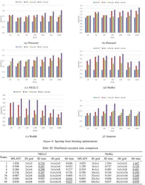
increasingly worse, while our blocking implementations can still achieve good performance.
Secondly, forNet f lix,Reddit, andAmazon, the speedup of our blocking implementations over SPLATT is lower at higher ranks. This is because all these three tensors have very large dimension sizes. MTTKRP on them with a large rank requires using very large numbers of blocks for both MB and RankB, and the overhead of blocking outweighs the benefits. As a result, blocking techniques can not work effectively for those tensors with very large ranks, and we see the speedup peak at lower ranks.
Thirdly, our blocking implementations achieve higher speedup on the real data sets than on the synthetic data sets. For the two synthetic data sets, speedup ranges from 1.07×to 2.02×, whereas for the four real data sets, speedup ranges from 1.00×to 3.54×. This is probably because there exist nice dense sub-structures in the real data sets, while the synthetic data sets have more random sparse patterns. Using blocking techniques, we can effectively take advantage of dense sub-structures in the real data and achieve better performance.
Lastly, we observe that RankB alone is typically not as effective as MB. However, it is more effective when combining RankB with MB. We also observe that speedup peaks at a rank of 32 for Reddit, and a rank of 128 for Amazon, despite the fact that Amazonhas larger dimension sizes. This may be due to Amazon having slightly higher density and larger nonzero clustering that can better benefit from the blocking techniques even when rank is large.
D. Distributed system results
Table III shows the performance of our distributed par-allel MTTKRP implementation and compares against the distributed SPLATT implementation forNELL2 andNet f lix. Our distributed implementation uses two different mecha-nisms to distribute data. The first mechanism, indicated by the column labeled 3D in the table, uses the same medium-grained decomposition method as SPLATT to distribute the data. SPLATT first assumes that there are p=q×r×s processors available, and attempts to partition each mode into q, r, and s blocks that achieves some level of load balancing. The process is as follows:
1) Randomly permute the mode order to eliminate potential load imbalance from the data collection process 2) Partition the first permuted mode into q blocks. The
block boundaries are determined greedily by adding slices to a block until it has at least nnzq nonzeros. 3) Repeat this process for the second and third mode.
The second mechanism, indicated by the column labeled 4Din the table, adds an extra dimension to processor grid by partitioning along the rank. We first determine an optimal partition count t along the rank, and then apply the 3D partitioning to the tensor by dividing it into pt =q0×r0×s0 partitions. Since the processors are partitioned intop=q0×
r0×s0×t grid, we call it the 4Dpartitioning. Note that each q0×r0×s0 partition contains the tensor in its entirety (i.e., there aret copies of the tensor among the processors). Also, this method requires an extra AllGather operation compared to the medium-grained decomposition method. However, the overhead is negligible (and included in our execution time).
As seen in Table III, our blocking implementation, whether it uses the 3Dor the 4D partitioning, always outperforms the baseline SPLATT implementations for all data sets. This is mainly attributed to the blocking methods applied locally on the partition of each processor. On 64 nodes, we achieve 1.4×and 1.6× for the NELL-2 and Net f lix data sets, respectively (taking the lowest execution time between 3Dand 4Dpartitioning mechanisms). The 4Dpartitioning outperforms performance the 3D. This is expected since the 4Dpartitioning allows each processor to retain more nonzeros (instead of nnzp, each processor has t∗nnzp ). As a result, it has less communication overheads and better scalability, compared to the 3Dpartitioning.
VII. CONCLUSION ANDFUTUREWORK
0.0 0.5 1.0 1.5 2.0 2.5
16 32 64 128 256 512 1024
Sp
ee
du
p
Rank
SPLATT MB RankB MB + RankB
(a)Poisson2
0.0 0.2 0.4 0.6 0.8 1.0 1.2 1.4 1.6 1.8
16 32 64 128 256 512 1024
Sp
ee
du
p
Rank
SPLATT MB RankB MB + RankB
(b)Poisson3
0.0 0.5 1.0 1.5 2.0 2.5
16 32 64 128 256 512 1024
Sp
ee
du
p
Rank
SPLATT MB RankB MB + RankB
(c) NELL-2
0.0 0.5 1.0 1.5 2.0 2.5 3.0 3.5
16 32 64 128 256 512 1024
Sp
ee
du
p
Rank
SPLATT MB RankB MB + RankB
(d)Netflix
0.0 0.5 1.0 1.5 2.0 2.5 3.0 3.5 4.0
16 32 64 128 256 512 1024
Sp
ee
du
p
Rank
SPLATT MB RankB MB + RankB
(e)Reddit
0.0 0.5 1.0 1.5 2.0 2.5
16 32 64 128 256 512 1024
Sp
ee
du
p
Rank
SPLATT MB RankB MB + RankB
(f)Amazon
Figure 6:Speedup from blocking optimizations
Table III:Distributed execution time comparison
Nodes
NELL2 Netflix
SPLATT 3D grid 3D time 4D grid 4D time SPLATT 3D grid 3D time 4D grid 4D time
1 1.028 1x1x2 0.718 1x1x1x2 0.826 3.025 2x1x1 1.554 1x1x1x2 1.447
2 0.540 1x1x4 0.367 1x1x1x4 0.423 1.158 4x1x1 0.727 1x1x1x4 0.720
4 0.286 2x1x4 0.208 1x1x1x8 0.217 0.519 8x1x1 0.403 1x1x1x8 0.401
8 0.138 2x2x4 0.107 1x1x1x16 0.124 0.256 16x1x1 0.194 1x1x1x16 0.190
16 0.087 2x2x8 0.058 1x1x2x16 0.065 0.113 32x1x1 0.103 2x1x1x16 0.100
32 0.056 4x2x8 0.043 1x1x4x16 0.034 0.083 32x2x1 0.056 4x1x1x16 0.055
64 0.030 4x4x8 0.028 2x1x4x16 0.022 0.048 64x2x1 0.037 8x1x1x16 0.030
more efficient by allowing each processor to retain more nonzeros without increasing the communication complexity.
However, we need to address the issue of finding the optimalblocking sizes for our various blocking techniques more effectively. Due to the inherently complex nature of high order sparse computation, finding the optimal sizes would require a more accurate model for data movement, as well as
an efficient heuristic to search through the parameter space. That is, a well designed autotuning framework would allow the work presented here to be practical to real applications.
ACKNOWLEDGMENT
REFERENCES
[1] T. G. Kolda and B. W. Bader, “Tensor decompositions and applications,” SIAM Review, vol. 51, no. 3, pp. 455–500, September 2009.
[2] N. D. Sidiropoulos, L. De Lathauwer, X. Fu, K. Huang, E. E. Papalexakis, and C. Faloutsos, “Tensor decomposition for signal processing and machine learning,”IEEE Transactions on Signal Processing, vol. 65, no. 13, pp. 3551–3582.
[3] U. Kang, E. Papalexakis, A. Harpale, and C. Faloutsos, “Gi-gatensor: Scaling tensor analysis up by 100 times - algorithms and discoveries,” inProceedings of the 18th ACM SIGKDD International Conference on Knowledge Discovery and Data Mining, ser. KDD ’12, 2012.
[4] S. Smith, N. Ravindran, N. D. Sidiropoulos, and G. Karypis, “Splatt: Efficient and parallel sparse tensor-matrix multi-plication,”29th IEEE International Parallel & Distributed Processing Symposium, 2015.
[5] J. H. Choi and S. V. N. Vishwanathan, “Dfacto: Distributed factorization of tensors,” inProceedings of the 27th Interna-tional Conference on Neural Information Processing Systems, ser. NIPS’14, 2014.
[6] R. Nishtala, R. W. Vuduc, J. W. Demmel, and K. A. Yelick, “When cache blocking of sparse matrix vector multiply works and why,”Applicable Algebra in Engineering, Communication and Computing, vol. 18, no. 3, pp. 297–311, 2007.
[7] A. Buluc¸ and J. R. Gilbert, “Parallel sparse matrix-matrix multiplication and indexing: Implementation and experiments,” SIAM Journal of Scientific Computing (SISC), vol. 34, no. 4, pp. 170 – 191, 2012.
[8] S. Smith and G. Karypis, “A medium-grained algorithm for dis-tributed sparse tensor factorization,”30th IEEE International Parallel & Distributed Processing Symposium, 2016.
[9] T. B. Rolinger, T. A. Simon, and C. D. Kriege, “Performance evaluation of parallelsparse tensor decomposition implemen-tations,” in Proceedings of the 6th Workshop on Irregular Applications: Architectures and Algorithms, ser. IA3 ’16. ACM, 2016.
[10] B. W. Bader, T. G. Kolda et al., “Matlab tensor toolbox version 2.6,” Available online, February 2015. [Online]. Available: http://www.sandia.gov/∼tgkolda/TensorToolbox/
[11] J. Li, C. Battaglino, I. Perros, J. Sun, and R. Vuduc, “An input-adaptive and in-place approach to dense tensor-times-matrix multiply,” in Proceedings of the International Conference for High Performance Computing, Networking, Storage and Analysis, ser. SC ’15. ACM, 2015, pp. 76:1–76:12.
[12] S. Smith and G. Karypis, “Tensor-matrix products with a compressed sparse tensor,” inProceedings of the 5th Workshop on Irregular Applications: Architectures and Algorithms. ACM, 2015, p. 7.
[13] S. Smith, J. Park, and G. Karypis, “Sparse tensor factoriza-tion on many-core processors with high-bandwidth memory,” 31st IEEE International Parallel & Distributed Processing Symposium (IPDPS’17), 2017.
[14] E. Solomonik, D. Matthews, J. Hammond, and J. Demmel, “Cyclops tensor framework: reducing communication and eliminating load imbalance in massively parallel contractions,” inParallel & Distributed Processing (IPDPS), 2013 IEEE 27th International Symposium on. IEEE, 2013, pp. 813–824.
[15] K. Shin and U. Kang, “Distributed methods for high-dimensional and large-scale tensor factorization,” in Proceed-ings of the 2014 IEEE International Conference on Data Mining, ser. ICDM ’14. IEEE Computer Society, 2014, pp. 989–994.
[16] O. Kaya and B. Uc¸ar, “Scalable sparse tensor decomposi-tions in distributed memory systems,” inProceedings of the International Conference for High Performance Computing, Networking, Storage and Analysis, ser. SC ’15. ACM, 2015, pp. 77:1–77:11.
[17] O. Kaya and B. Uc¸ar, “Parallel cp decomposition of sparse tensors using dimension trees,” Ph.D. dissertation, Inria-Research Centre Grenoble–Rhˆone-Alpes, 2016.
[18] B. W. Bader and T. G. Kolda, “Efficient matlab computations with sparse and factored tensors,” SIAM JOURNAL ON SCIENTIFIC COMPUTING, vol. 30, no. 1, pp. 205–231, 2007.
[19] V. Sharan and G. Valiant, “Orthogonalized als: A theoretically principled tensor decomposition algorithm for practical use,” arXiv preprint arXiv:1703.01804, 2017.
[20] S. Williams, A. Waterman, and D. Patterson, “Roofline: An in-sightful visual performance model for multicore architectures,” Commun. ACM, vol. 52, no. 4, pp. 65–76, Apr. 2009.
[21] K. Czechowski, “Diagnosing performance limitations in hpc applications,” Ph.D. dissertation, Georgia Institute of Technol-ogy, 2015.
[22] J. Sun, D. Tao, and C. Faloutsos, “Beyond streams and graphs: Dynamic tensor analysis,” inProceedings of the 12th ACM SIGKDD International Conference on Knowledge Discovery and Data Mining, ser. KDD ’06. ACM, 2006.
[23] D. M. Dunlavy, T. G. Kolda, and E. Acar, “Temporal link prediction using matrix and tensor factorizations,”ACM Trans. Knowl. Discov. Data, vol. 5, 2011.
[24] S. Hansen, T. Plantenga, and T. G. Kolda, “Newton-based optimization for kullback–leibler nonnegative tensor factor-izations,”Optimization Methods Software, vol. 30, no. 5, pp. 1002–1029, 2015.
[25] E. C. Chi and T. G. Kolda, “On tensors, sparsity, and nonneg-ative factorizations,” SIAM J. Matrix Analysis Applications, vol. 33, pp. 1272–1299, 2012.
[26] J. Bennett, S. Lanning, and N. Netflix, “The netflix prize,” in In KDD Cup and Workshop in conjunction with KDD, 2007.
[27] A. Carlson, J. Betteridge, B. Kisiel, B. Settles, E. R. Hr-uschka, Jr., and T. M. Mitchell, “Toward an architecture for never-ending language learning,” in Proceedings of the Twenty-Fourth AAAI Conference on Artificial Intelligence, ser. AAAI’10, 2010.
[28] J. McAuley and J. Leskovec, “Hidden factors and hidden topics: Understanding rating dimensions with review text,” in Proceedings of the 7th ACM Conference on Recommender Systems, ser. RecSys ’13. ACM, 2013.