Adaptive backstepping control of tracked robot running trajectory based
on real-time slip parameter estimation
En Lu
1,2, Zheng Ma
1*, Yaoming Li
1, Lizhang Xu
1, Zhong Tang
1(1. School of Agricultural Equipment Engineering, Jiangsu University, Zhenjiang, Jiangsu 212013, China; 2. World Precise Machinery (China) Co., Ltd, World Industrial Park, Picheng Town, Danyang, Jiangsu 212311, China)
Abstract: To ensure the stable driving of tracked robots in a complex farmland environment, an adaptive backstepping control method for tracked robots was proposed based on real-time slip parameter estimation. According to the kinematics analysis method, the kinematic model of the tracked robot was established, and then, its pose error differential equation was further obtained. On this basis, the trajectory tracking controller of the tracked robot was designed based on the backstepping control theory. Subsequently, according to the trajectory tracking error of the tracked robot, the back propagation neural network (BPNN) was used to adaptively adjust the control parameters in the backstepping controller, and the inputs of the BPNN are the trajectory tracking error xe, ye, θe. After that, the soft-switching sliding mode observer (SSMO) was designed to identify the slip parameters during the running of the tracked robot. And then the parameters were compensated into the adaptive backstepping controller to reduce the trajectory tracking error. The simulation results show that the proposed adaptive backstepping control method with SSMO can improve the accuracy of the trajectory tracking control of the tracked robot. Additionally, the designed SSMO can accurately estimate the slip parameters.
Keywords: tracked robot, trajectory control, adaptive backstepping control, neural networks, slip parameter, sliding mode observer
DOI: 10.25165/j.ijabe.20201304.5739
Citation: Lu E, Ma Z, Li Y M, Xu L Z, Tang Z. Adaptive backstepping control of tracked robot running trajectory based on real-time slip parameter estimation. Int J Agric & Biol Eng, 2020; 13(4): 178–187.
1 Introduction
The tracked robots have the advantages of the large driving force, small grounding pressure and good passability, and can be well adapted to special terrain. They are widely used in military vehicles, agricultural machinery, engineering machinery, etc. Therefore, the research on trajectory tracking control of tracked robots has received more and more attention[1,2]. In tracked robots, the interaction between the tracks, wheels, and soil can cause slippage, slip-rotation, subsidence, etc. Moreover, there are errors and gaps in the mechanical structure, and the control system also has uncertain factors. These cause a certain deviation between the actual running trajectory and the reference trajectory and seriously affect the actual work performance of the tracked robot[3].
Bian et al.[4] established the kinematic model and trajectory tracking dynamic error model of the tracked robot, and a state feedback control law was proposed based on the Lyapunov stability theory. The designed control law can realize linear trajectory tracking and circular trajectory tracking quickly and effectively,
Received date: 2020-02-17 Accepted date: 2020-03-18
Biographies:En Lu, PhD, Assistant Researcher, research interests: intelligent agricultural robotics, complex system modeling, and nonlinear control. Email: [email protected]; Yaoming Li, PhD, Professor, research interests: intelligent agricultural machinery. Email: [email protected]; Lizhang Xu, PhD, Researcher, research interests: intelligent agricultural machinery, Email:[email protected]; Zhong Tang, PhD, Associate Researcher, research interests: intelligent agricultural machinery. Email: [email protected].
*Corresponding author: Zheng Ma, PhD, Associate Researcher, research interest: intelligent agricultural machinery. School of Agricultural Equipment Engineering, Jiangsu University, No.301 Xuefu Road, Zhenjiang 212013, China. Tel: +86-18796005357, Email: [email protected].
and it has a better control effect. Han et al.[5] considered the trajectory tracking control problem of tracked robots under restricted motion conditions, the finite-time control law of the steering angular velocity and the sliding mode control law of the longitudinal linear velocity were designed. Jiao et al.[6] established a cascade system based on the motor drive equation and vehicle kinematic equation and proposed an adaptive sliding mode tracking control method. In order to solve the path tracking control problem of differential steering tracked vehicles, Wang et al.[7] proposed a vertical and horizontal cooperative tracking control
method based on the two-layer driver model. Asif et al.[8]
proposed a new adaptive sliding mode dynamic controller with an integrator for non-complete wheeled mobile robots. The simulation results showed that the control scheme has zero steady-state error, fast error convergence and robustness in the presence of disturbances and uncertainties. Yokoyama et al.[9] designed an adaptive controller for the trajectory tracking problem of mobile robots, which combined the advantages of the backstepping method and immersion and invariant control (I&I) method. Wu et al.[10] proposed a hybrid robust control algorithm based on backstepping kinematics control and fuzzy sliding mode robust dynamics control, which solved the trajectory tracking control problem of the mobile robot model under uncertainties and external interferences.
vehicle, Xiong et al.[11] used the Levenberg-Marquardt algorithm to iteratively solve the slip parameters, and combined with the given control sequence to predict the trajectory of the tracked vehicle for a period of time in the future. Based on the kinematic model, Zhu et al.[12] designed a sliding mode observer (SMO) with Lyapunov stability for estimating the slippage parameters, and optimized the gain of the SMO using the non-dominated classification particle swarm optimization algorithm to improve the accuracy of the estimation results. Bei et al.[13] designed a low-pass filter to improve the chattering problem in the SMO. Song et al.[14,15] designed the SMO and the extended Kalman filter observer to estimate the slip parameters of the tracked robot, the simulations and experiments verified that the two methods can accurately estimate the slip parameters. Iossaqui et al.[16] established the kinematic model by approximating the tracked robot to a differential wheeled robot. Based on this, an adaptive nonlinear fed back control law with slip compensation was proposed to realize the trajectory tracking control by using the update rules of compensating slip. Zhao et al.[17] proposed an SMO based on the longitudinal dynamics model of the independent four-wheel-drive electric vehicle. The tire slip and vehicle speed under unknown road surfaces were achieved by measuring electromagnetic torque and angular velocity of four motors.
In this paper, an adaptive backstepping control of tracked robot running trajectory based on real-time slip parameter estimation was proposed based on the above research results. Firstly, the trajectory tracking controller of the tracked robot was designed based on the backstepping method. In order to improve the adaptive ability of the tracked robot under different actual running conditions, the back propagation neural network (BPNN) was used to adaptively adjust the control parameters in the backstepping controller. In addition, the strategy of “identification first, compensation later” was adopted to eliminate the influence of slides of the tracked robot during the running process. The SMO was designed to identify the slip parameters of the tracked robot in this paper. The soft switching function was used to replace the traditional switching function to avoid the chattering phenomenon of the sliding mode surface, and the effects of interferences were further reduced by the low-pass filter. Then the identified slip parameters were compensated into the control system. The effectiveness of the proposed method was verified by simulation analysis.
2 Kinematic model of the tracked robot
First, the following assumptions were represented for the tracked robot:
(1) The track length is fixed and the grounding part is not deformed;
(2) The ground is flat and the track grounding pressure is even; (3) The centroid of the tracked robot is located at the center of the vehicle.
As shown in Figure 1, the schematic diagram of the planar motion of the tracked robot in the global XOY coordinate system, xoy is the local coordinate system attached to the vehicle, the origin o is at the centroid of the tracked robot, and the x-axis is the forward direction of the tracked robot; θ is the heading angle of the tracked robot, rad; and b is the center distance of the two tracks, m.
Assume that the theoretical speeds of the left and right tracks are vL and vR respectively, m/s; and v is the velocity of the tracked robot, m/s; ω is angular velocity of the tracked robot, rad/s; then,
1 1 2 2 1 1 L R v v v b b (1)
Therefore, in the global XOY coordinate system, the kinematic equation of the tracked robot that does not consider the influence of the slip factors can be expressed as[6]:
cos 0
= sin 0
0 1 X v Y (2)
If the turning radius of the tracked robot is assumed as R, m; the current turning radius of the tracked robot can be calculated from the equation v=Rω:
2
L R
L R
v b v v
R
v v
(3)
It can be seen from Equation (3) that when vL=vR, the rotational angular velocity ω=0 of the tracked robot and the turning radius are infinite, the trajectory of the tracked robot can be approximated as a straight line; when vL=−vR, the turning radius of the tracked robot is equal to 0, and the tracked robot rotates around the center o.
Figure 1 Schematic diagram of the planar motion of the tracked robot
3 Design of adaptive backstepping controller
As shown in Figure 1, the tracked robot runs to the point P after the time Δt from the point S, and the pose of the tracked robot in the global XOY coordinate system is represented by P=[X, Y, θ]T, the motion velocity is q=[v, ω]T. The pose and motion velocity of the reference trajectory Pr point are expressed as Pr=[Xr, Yr, θr]T, qr=[vr, ωr]T, respectively. Therefore, the pose error of the tracked robot under the local xoy coordinate system is expressed as pe=[xe, ye, θe]
T
, and it can be obtained as:
cos sin 0
sin cos 0
0 0 1
e r
e r
e r
x X X
y Y Y
(4)
Deriving Equation (4) and combining Equation (2) can obtain the pose error differential equation of the tracked robot as[4]:
cos
sin
e e r e
e e r e
e r
x y v v
y x v
(5)
Combined with Equation (4), the following Lyapunov function is designed based on the backstepping control theory:
2 2 1
2
1 1
( + ) (1 cos )
2 e e e
V x y
k
(6)
1 2 2 2 2 1 sin 1
( cos ) ( sin ) ( )sin
1 1
cos sin sin sin (7)
e e e e e e
e e r e e e r e r e
e r e e e r e r e e
V x x y y
k
x y v v y x v
k
x v x v y v
k k
The auxiliary control input is selected as[18]:
1
2 3
cos
sin
r e e
r r e r e
v v k x
k v y k v
(8)
Substituting Equation (8) into Equation (7) we can obtain:
3
2 2
1 1
2 sin
e r e
k
V k x v
k
(9)
Where, when k1>0, k2>0, k3>0 and vr>0, V10. It indicates that the designed control law meets the theoretical Lyapunov stability condition, thus ensuring the asymptotic stability of the system in the global sense.
The tracked robot is a multi-variable strong coupling system, the trajectory tracking effects are affected by vehicle acceleration and deceleration, sharp turns and the ground. When the trajectory control of the tracked robot is carried out using the backstepping controller designed above, and the control effect may be somewhat unsatisfactory, and may even cause system instability[19]. This is because the fixed control parameters k1, k2, and k3 in the controller
cannot cope with such nonlinear, strong coupling and complex environments. The Neural network has arbitrary nonlinear expression
ability. Therefore, this paper combines the multi-dimensional function mapping and learning ability of BPNN to adjust the control parameters of the backstepping controller in real-time, and constitutes the trajectory tracking controller of the tracked robot with adjustable parameters, strong adaptability and robustness.
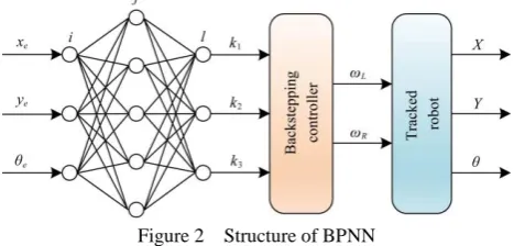
Figure 2 Structure of BPNN
According to Figure 2, a 3-layer BPNN structure (3-5-3) is constructed. The inputs of the input layer are xe, ye, θe. The hidden layer has 5 nodes, and the outputs of the output layer are the control parameter k1, k2, k3 in the backstepping controller. The
specific design steps of BPNN are as follows[20]. The inputs of the input layer can be expressed as:
(1) ( ) i
O xi i (10)
where, the upper corner (1) represents the input layer; i=1, 2, 3; xi(1)=xe, xi(2)=ye, xi(3)=θe.
The inputs and outputs of the hidden layer can be expressed as: 3
(2) (2) (1)
0 ( )
j ji i
i
net k w O
(11)(2) (2)
( ) ( ( ))
j j
O k f net k (12)
where, the upper corner (2) represents the hidden layer; j =1, 2, 3, 4, 5; wij(2)is the hidden layer weighting coefficient.
The positive and negative symmetric Sigmoid function is selected as the activation function of the hidden layer neurons, and
shown as follows:
( ) tanh( )
x x
x x
e e
f x x
e e
(13)
The inputs and outputs of the output layer can be expressed as: 5
(3) (3) (2)
0
( ) j ( )
l lj
j
net k w O k
(14)(3) (3)
( ) ( ( ))
l l
O k g net k (15) where, the upper corner (3) represents the output layer; l =1, 2, 3.
The output nodes of the output layer correspond to three tunable parameters k1, k2, k3 in the backstepping controller, scilicet
O1(3)(k)=k1, O2(3)(k)=k2, O3(3)(k)=k3. Since k1, k2, and k3 are all
greater than 0, the non-negative Sigmoid function is selected as the activation function of the output layer neurons and shown as follows:
1
( ) (1 tanh( ))
2
x
x x
e
g x x
e e
(16)
The performance indicator function is selected as:
2 2 2
3
2
1
1 1 1
( ) ( ) ( ) ( ) ( ) ( ) ( )
2 2 2
( ) ( ) (17)
r r r
p p
p
E k X k X k Y k Y k k k
r k y k
The gradient descent method is chosen to correct the weight coefficient of the neural network, that is, to perform search adjustment on the negative gradient direction of the weighting coefficient, and to add an inertial term that searches quickly converge globally. Therefore, the correction equation for the weight coefficient of the neural network is shown as follows.
(3) (3)
(3) ( )
( ) ( 1)
lj lj
lj E k
w k w k
w
(18)
where, η is the learning rate and α is the inertia coefficient. Thus,
(3) (3)
(3) (3) (3) (3)
( )
( ) ( ) ( ) ( )
( ) ( ) ( ) ( ) ( )
p l l
p
lj l l lj
y k
E k E k O k net k
w k y k O k net k w k
(19)
Since (3)( ) ( ) p l y k O k
is unknown in Equation (19), the
approximation is replaced by the sign function
(3) (3)
( +1) ( )
sgn
( ) ( 1)
p p
l l
y k y k
O k O k
. The calculation error caused by the
above replacement can be compensated by adjusting the learning rate η, then the Equation (19) can be rewritten as[21]:
3
(3) (3) (3)
1
(3) (2)
( +1) ( )
( )
( ) ( ) sgn
( ) ( ) ( 1)
( ( )) ( )
p p
p p
p
lj l l
j l
y k y k
E k
r k y k
w k O k O k
g net k O k
(20)where, g ( ) g x( )(1g x( )). Assume:
(3) (3)
(3) (3)
( +1) ( )
( ) ( ) sgn ( ( ))
( ) ( 1)
p p
p p
lp l
l l
y k y k
r k y k g net k
O k O k
(21)
At this time you can get: 3
(3) (3) (2) (3)
1
( ) j ( ) ( 1)
lj lp lj
p
w k O k w k
(22)Similarly, the learning algorithm of the hidden layer weighting coefficient can be obtained:
(2) (2) (1) (2)
( ) ( ) ( ) ( 1)
ji jp i ji
w k k O k w k
(23)
3 3
(2) (2) (3) (3)
1 1
( ) '( ( )) ( )
j j lp lj
p h
k f net k w k
where, 2 ( ) (1 ( )) / 2
f f x .
Finally, the complete adaptive backstepping controller of the tracked robot is shown in Figure 3.
Figure 3 Structure diagram of adaptive backstepping controller of the tracked robot
4 Design of SSMO
In the actual motion control of the tracked robot, there are the slides in the direction of travel and lateral. They cause the difference between the amount of output control and the amount of desired control, resulting in errors in the trajectory tracking control. This paper designs an SSMO to observe the slip parameters of the tracked robot, and they are used to compensate for the trajectory tracking control error which is caused by the slides.
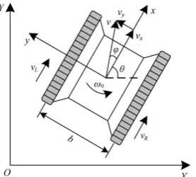
The schematic diagram of the tracked robot under slippage and slip-rotation conditions is shown in Figure 4. In the local xoy coordinate system, the lateral slip-rotation angle of the tracked robot is φ, and the actual motion speeds of the tracked robot are vx and vy on the x-axis and the y-axis respectively. The slip ratios of the tracked robot in the traveling direction on the left and right tracks are iL, iR, and can be expressed as[22]:
L x L L R x R R r v i r r v i r (25)
where, ωL and ωR are the angular velocities of the left and right drive wheels, rad/s; r is the radius of the drive wheel, m.
Figure 4 Schematic diagram of tracked robot under slippage and slip-rotation conditions
According to the kinematics analysis method and considering the influence of the slides (slippages and slip-rotation), the kinematic equation of the tracked robot under the local xoy coordinate system can be established as follows:
(1 ) (1 )
2
tan (1 ) (1 ) tan
2
(1 ) (1 )
L L R R x
x L L R R
L L R R
r
x i i v
r
y v i i
r i i b (26)
Through the transformation matrix of the local xoy coordinate system to the global XOY coordinate system[23], the kinematic
equation of the tracked robot in the global XOY coordinate system can be obtained and shown as follows.
cos tan sin
sin tan cos
[2 2 (1 )] / [ 2 2 (1 )] /
x x
x x
x L L x R R
X v v
Y v v
v r i b v r i b
(27)
Therefore, the SMO is built, and shown as follows.
1 2 1 3 ˆ cos 2 ˆ 2 ˆ x smo x smo x smo
X v u
v u b v u b (28)
The differential equation of observation error is shown as follows. 1 2 1 3 tan sin 2 (1 ) 2 (1 ) x smo
L L smo
R R smo
X v u
r i u b r i u b (29)
where, the superscript ~ represents the error terms, XXXˆ , ˆ
, 1 1 ˆ1.
The sliding mode surfaces are defined as ssmo1XXˆ ,
2 ˆ
smo
s , ssmo3 1 ˆ1, respectively. The inputs of the SMO can be expressed as:
1 1 1 2 1
2 3 2 2 2
3 4 3 2 3
sgn( ) ( )
sgn( ) ( )
sgn( ) ( )
smo g smo g smo
smo g smo g smo
smo g smo g smo
u k s k s
u k s k s
u k s k s
(30)
where, kg1, kg2, kg3, kg4 are sliding mode gain coefficients and they
are all greater than 0, and their values need to meet the reachability and existence conditions of the designed SMO.
By selecting the appropriate sliding mode gain coefficients kg1,
kg2, kg3, kg4, the observed error differential in Equation (29) will
converge to zero in a finite time, so the slip parameters of the tracked robot can be obtained and shown as follows[14].
1 1 1 1
3 2 2 2
4 3 4 3
sgn( )
arctan
sin
1 ( sgn( ) )
2
1 ( sgn( ) )
2
g smo g smo
x
L g smo g smo eq
L
R g smo g smo eq
R
k s k s
v
b
i k s k s
r b
i k s k s
r (31)
where, represents the estimated value of the slip-rotation angle φ; iL represents the estimated value of the left track slip ratio iL,
and iR represents the estimated value of the right track slip ratio
iR. Proof:
According to the sliding mode surfaces ssmo1, ssmo2, ssmo3 and
Equation (29), the following Lyapunov equation is selected:
Among them, the first derivative of Vsmo1 can be expressed as:
1 1 1
1
2
1 1 1 1 2 1
1 1 1 1
ˆ
( )
tan sin sgn( )
tan sin sgn( )
smo smo smo
smo
x smo g smo smo g smo
x smo g smo smo
V s s
s X X
v s k s s k s
v s k s s
(33)
where, when kg1vxtan sin , Vsmo10 . Similarly, the following can be obtained, when kg3| 2rL(1iL) / |b , Vsmo20; when kg4| 2rR(1iR) / |b , Vsmo30. Therefore, the designed SMO is progressively stable by reasonably selecting kg1, kg3 and kg4,
the estimation of the slip parameters of the tracked robot can be guaranteed.
Although the designed SMO can accurately estimate the slip parameters of the tracked robot, the switching function sgn in the SMO will cause high-frequency chattering of the system, thereby reducing the observation effect of the slip parameters. In order to suppress the inherent chattering phenomenon near the sliding mode surface in the SMO, the soft-switching sliding mode function with a variable boundary is used to replace the traditional switching function in the SMO and obtains the SSMO[24]. The soft-switching sliding mode function is shown as follows.
sgn( ) | |
sat( )
sin( ) | |
2
smo smo
smo smo
smo
s s
s s
s
(34)
where, ssmo corresponds to the sliding mode surfaces ssmo1, ssmo2,
ssmo3; ξ is the thickness of the variable boundary layer.
The curves of the traditional switching function and the soft-switching sliding mode function with variable boundary are shown in Figure 5.
a. Traditional switching function sgn b. Soft-switching sliding mode function with variable boundary sat Figure 5 Comparison curves of two sliding mode switching
functions
Finally, the slip parameters identified by the SSMO are compensated into the adaptive backstepping controller to improve the accuracy of the trajectory tracking control of the tracked robot.
5 Simulation analysis
The simulation parameters are as follows: The distance between the two tracks of the tracked robot is b = 0.5 m, the radius of the drive wheel is r = 0.1 m, the control interval is ts = 0.1 s, the speed range of the left and right drive wheels are −0.5-0.5 m/s, the reference trajectories are straight lines and the arc, and the initial values of the control parameters in the backstepping controller are k1=5, k2=50, and k3=10, respectively.
The reference trajectory of the tracked robot is the combination of straight lines and arcs. It is a straight line trajectory at 0-10 s, the slope is π/3 rad, the reference inputs are vr=0.2 m/s and ωr= 0 rad/s. After that, it is a circular trajectory at 10-20 s, the radius is rc=1 m, the reference inputs are vr=0 m/s and ωr=π/30 rad/s.
Finally, it is a straight line trajectory at 20-30 s, the slope is 0 rad, the reference inputs are vr=0.2 m/s and ωr=0 rad/s. In the global XOY coordinate system, the poses of the starting point of the theoretical trajectory are Xr(0)=1 m, Yr(0)=0 m, θr(0)=π/3 rad, and the initial poses of the tracked robot are X(0)=1.2 m, Y(0)=0.2 m, θ(0)=π/2 rad.
In order to further reduce the impact of system disturbances on the SSMO, the low-pass filter is selected to filter the observations, the equation is as follows[20].
1 ( )
0.04 1
Q s s
(35)
The low-pass filter shown in Equation (35) is discretized using the Tustin transform.
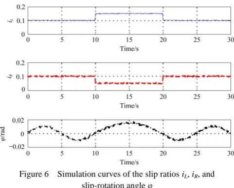
In order to analyze the effectiveness of the proposed method, it is necessary to simulate the slip parameters of the tracked robot. The simulation curves of the slip ratios iL, iR of left and right tracks and slip-rotation angle φ are shown in Figure 6.
Figure 6 Simulation curves of the slip ratios iL, iR, and slip-rotation angle φ
5.1 Influence of slide effect on trajectory tracking control
The trajectory tracking control of the tracked robot is simulated by the backstepping controller, which is divided into two cases: no-slip and existing slip, the results are shown in Figure 7. Figure 7a shows the trajectories of the tracked robot. It shows that there are deviations between the actual running trajectory and the reference trajectory whether there is a slide effect or not during the running of the tracked robot. The deviation value is larger between the actual running trajectory and the reference trajectory when there is the slide effect, and trajectory errors (xe, ye, θe) are shown in Figure 7b. Thus, the slide effect of the tracked robot will have an adverse influence on its trajectory tracking control, and it cannot be ignored in the control. Figure 7c shows the auxiliary control values in the backstepping controller. It can be seen that the tracked robot needs larger control values when there is a slide effect. Figure 7d shows the speeds of the left and right tracks. It can be seen that the speed fluctuations of the left and right tracks are greater when there is the slide effect.
5.2 Control effect simulation of trajectory tracking controller
tracking control error during the turning of the tracked robot. The proposed adaptive backstepping controller improves the effects of trajectory tracking control, but still cannot eliminate the influence of the slide effect on trajectory tracking control. Figure 8c shows the auxiliary control values in the trajectory tracking controller. It can be seen that the proposed adaptive backstepping controller has a faster control response. Figure 8d shows the speeds of the left and right tracks. Figure 8e shows the change trends of controller parameters (k1, k2, k3) adjusted by the BPNN according to the
running state of the tracked robot.
5.3 Observation of slip parameters
The observation results of the slip parameters of the tracked
robot are shown in Figure 9. Figure 9a shows the sliding mode surfaces in the SSMO, it can be seen that the chattering of the sliding mode surfaces is smaller after the optimization by the soft sliding mode switching function. It illustrates that soft sliding mode switching function can eliminate the chattering phenomenon in the SSMO, and guarantee the stability of the system. Figure 9b shows the observation results of the slip ratio iL of the left track. Figure 9c shows the observation results of the slip ratio iR of the right track. Figure 9d shows the observation results of the slip-rotation angle φ. It can be seen from Figures 9b, 9c and 9d, the deigned SSMO can accurately observe the slip parameters of the tracked robot.
a. Trajectories of the tracked robot b. Trajectory errors
c. Auxiliary control values d. Speeds of left and right tracks
Note: Ref_ trajectory indicates the reference trajectory; BC_noslip indicates the control results of backstepping controller in the without slip state; BC_slip indicates the control results of backstepping controller in the slip state.
Figure 7 Simulation analysis of the influence of slip parameters on trajectory tracking control
c. Auxiliary control values d. Speeds of left and right tracks
e. Controller parameters k1, k2, k3
Note: Ref_ trajectory indicates the reference trajectory; BC_slip indicate the control results of backstepping controller in the slip state; ABC_slip indicate the control results of adaptive backstepping controller in the slip state; k1 indicates the change changing trend of control parameter k1 in the adaptive backstepping controller; k2indicates the change changing trend of control parameter k2 in the adaptive backstepping controller; k3 indicates the changing trend of control parameter k3 in the adaptive backstepping controller.
Figure 8 Simulation comparison curves of backstepping controller and adaptive backstepping controller
a. Sliding mode surfaces b. Observation results of the slip ratio iL of left track
c. Observation results of the slip ratio iR of right track d. Observation results of the slip-rotation angle φ
Note: iL, iR, and φ indicate the actual values of the slip parameters iL, iR, and φ of the tracked robot, respectively; iLO, iRO, and φOindicate the observations of the slip parameters iL, iR, and φ of the tracked robot, respectively.
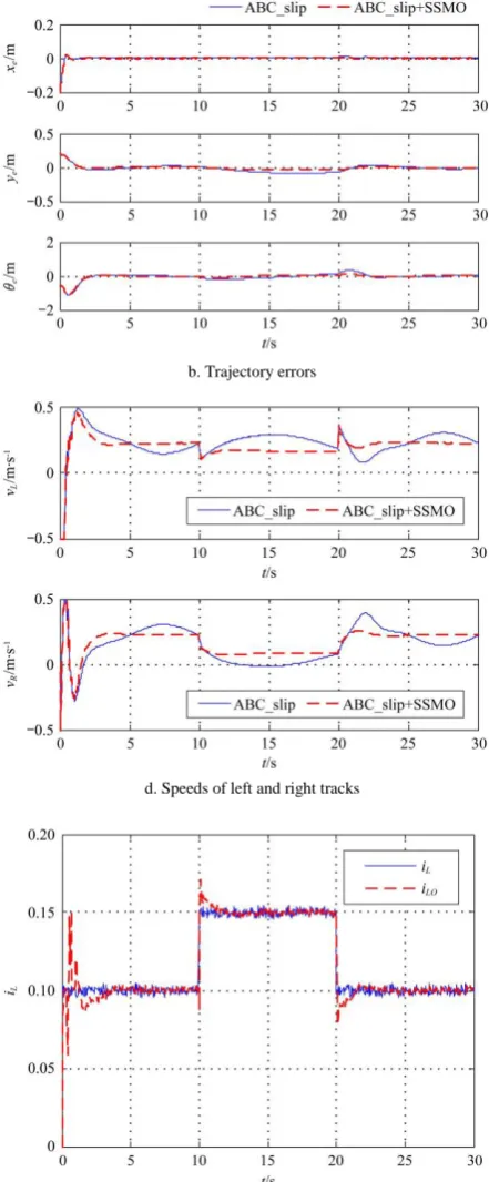
5.4 Simulation of adaptive backstepping controller with SSMO
The simulation results of the adaptive backstepping controller with SSMO are shown in Figure 10. Figure 10a shows the trajectories of the tracked robot and Figure 10b shows the trajectory errors (xe, ye, θe). It can be seen from Figures 10a and 10b, the adaptive backstepping controller with SSMO effectively improves the trajectory tracking accuracy of the tracked robot, especially when it turns. It illustrates that the tracked robot can better be adapted to the complex working environment by compensating the identified slip parameters into the adaptive backstepping controller. Figure 10c shows the auxiliary control values in the adaptive backstepping controller. Figure 10d shows the speeds of the left
and right tracks. Figure 10e shows the sliding mode surfaces in the SSMO. Figure 10f shows the observation results of the slip ratio iL of the left track. Figure 10g shows the observation results of the slip ratio iR of the right track. Figure 10h shows the observation results of the slip-rotation angle φ. It can be seen from Figure 10e, Figure 10f, Figure 10g and Figure 10h, the deigned SSMO can accurately observe the slip parameters of the tracked robot. Figure 10i shows the controller parameters (k1, k2,
k3) adjusted by the BPNN according to the running state of the
tracked robot. Compared with Figure 8e, the trends of parameter changes are more gradual, which also illustrates the effectiveness of the proposed adaptive backstepping controller with SSMO of the tracked robot.
a. Trajectories of the tracked robot b. Trajectory errors
c. Auxiliary control values d. Speeds of left and right tracks
g. Observation results of the slip ratio iR of right track h. Observation results of the slip-rotation angle φ
i. Controller parameters k1, k2, k3
Note: Ref_ trajectory indicates the reference trajectory; ABC_slip indicate the control results of adaptive backstepping controller in the slip state; ABC_slip+SSMO indicate the control results of adaptive backstepping controller with SSMO in the slip state; iL, iR, and φ indicate the actual values of the slip parameters iL, iR, and φ of the tracked robot, respectively; iLO, iRO, and φO indicate the observations of the slip parameters iL, iR, and φ of the tracked robot, respectively; k1 indicates the changing trend of control parameter in the adaptive backstepping controller with SSMO; k2 indicates the changing trend of control parameter k2in the adaptive backstepping controller with SSMO; k3 indicates the changing trend of control parameter k3 in the adaptive backstepping controller with SSMO.
Figure 10 Simulation results of the adaptive backstepping controller with SSMO
6 Conclusions
In this study, an adaptive backstepping control method for tracked robots based on real-time slip parameter estimation is presented. The adaptive backstepping control method inherits the advantages of the backstepping control method and introduces the learning ability of the BPNN to adjust the control parameters in the backstepping controller online according to the running state of the tracked robot. The slip parameters of the tracked robot are observed by the designed SSMO, and the observations are compensated into the adaptive backstepping controller to reduce the effects of slide effect. Finally, the performance of the designed adaptive backstepping controller with SSMO is investigated through numerical simulations.
The simulation analysis of the influence of the slide effect shows that the slide effect of the tracked robot has a bad influence on its trajectory tracking control, and its influence cannot be ignored in the control. The simulation comparison of the backstepping controller and adaptive backstepping controller shows that the adaptive backstepping controller achieves better control effects, especially on the linear trajectories. But there is still a large trajectory tracking control error during the turning of the tracked robot, and it illustrates that the influence of slide effect on trajectory tracking control is not eliminated. The observation
results of the slip parameters of the tracked robot show that the chattering of the sliding mode surfaces is smaller after the optimization by the soft sliding mode switching function, and the deigned SSMO can accurately observe the slip parameters of the tracked robot. Finally, the simulation results of the adaptive backstepping controller with SSMO show that the proposed method effectively improves the accuracy of the trajectory tracking control of the tracked robot, especially when it turns. It illustrates that the tracked robot can better be adapted to the complex working environment by compensating the identified slip parameters into the control system.
Acknowledgements
[References]
[1] Chen S Y, Chen W J. Review of tracked mobile robots. Mechanical and Electrical Engineering Magazine, 2007; (12): 109–112. (in Chinese) [2] Guo T Y, Guo J L, Huang B, Peng H. Power consumption of tracked and
wheeled small mobile robots on deformable terrains–model and experimental validation. Mechanism & Machine Theory, 2019; 133: 347–364.
[3] Zeng Q H, Ma X J, Yuan D, Liu C G. Motion decoupling and variable structure control of dual-motor electric drive tracked vehicle. Control Theory & Applications, 2015; 32(8): 1080–1089. (in Chinese)
[4] Bian Y M, Yang M, Liu Y C, Yang G. Research on trajectory tracking control of a tracked mobile robot. Chinese Journal of Construction Machinery, 2018; 16(3): 189–193, 206. (in Chinese)
[5] Han J, Ren G Q, Li D W. Trajectory tracking control for tracked mobile robot with moving limitation. Computer Measurement & Control, 2017; 25(12): 86–89. (in Chinese)
[6] Jiao J, Chen J, Qiao Y, Wang W Z, Wang M S, Gu L C, et al. Adaptive sliding mode control of trajectory tracking based on DC motor drive for agricultural tracked robot. Transactions of the CSAE, 2018; 34(4): 64–70. (in Chinese)
[7] Wang B Y, Gong J W, Gao T Y, Zhang R Z, Chen H Y, Xi J Q. Longitudinal and lateral path following coordinated control method of tracked vehicle based on double-layer driver model. Acta Armamentarii, 2018; 39(9): 1675–1682. (in Chinese)
[8] Asif M, Khan M. J, Cai N. Adaptive sliding mode dynamic controller with integrator in the loop for nonholonomic wheeled mobile robot trajectory tracking. International Journal of Control, 2014; 87(5): 964–975. [9] Yokoyama M, Ikarashi J, Okawa A. Adaptive control of a skid-steer
mobile robot with uncertain cornering stiffness. Mechanical Engineering Journal, 2015; 2(4): 15–00040. doi: 10.1299/mej.15-00040.
[10] Wu X, Jin P, Zou T, Qi Z, Xiao H, Lou P. Backstepping trajectory tracking based on fuzzy sliding mode control for differential mobile robots. J Intell Robot Syst, 2019; 96: 109–121.
[11] Xiong G M, Lu H, Guo K H, Chen H Y. Research on trajectory prediction of tracked vehicles based on real time slip estimation. Acta Armamentarii, 2017; 38(3): 600–607. (in Chinese)
[12] Zhu L, Guo J, Liu G F. Slip estimation method of track robot. Journal of Central South University (Science and Technology), 2013; 44(8): 3173–3178. (in Chinese)
[13] Bei X Y, Ping X L, Gao W Y. Trajectory tracking control of wheeled mobile robots under longitudinal slipping conditions. China Mechanical Engineering, 2018; 29(16): 1958–1964. (in Chinese)
[14] Song Z. B, Zweiri Y. H, Seneviratne L. D, Althoefer K. Non-linear observer for slip estimation of skid-steering vehicles. Proceedings 2006 IEEE International Conference on Robotics and Automation, Orlando: IEEE, 2006; pp.1499–1504.
[15] Song Z B, Song X J, Altheoer K, Zweiri Y, Seneviratne L. Non-linear observer for slip parameter estimation of unmanned wheeled vehicles. 2007 IFAC Proceedings Volumes, Harbin: IEEE, 2007; pp.458–463. [16] Iossaqui J G, Camino J F, Zampieri D E. A nonlinear control design for
tracked robots with longitudinal slip. IFAC Proceedings Volumes, 2011; 44(1): 5932–5937.
[17] Zhao Y, Tian Y T, Lian Y F, Hu L L. A sliding mode observer of road condition estimation for four-wheel-independent-drive electric vehicles. Proceeding of the 11th World Congress on Intelligent Control and Automation, Shenyang: IEEE, 2014; pp.4390–4395.
[18] Kanayama Y, Kimura Y, Miyazaki F, Noguchi T. A stable tracking control method for an autonomous mobile robot. Proceedings, IEEE International Conference on Robotics and Automation, Cincinnati: IEEE, 1990; 1: pp.384–389.
[19] Qu Y, Ning D, Lai Z C, Cheng Q, Mu L N. Neural networks based on PID control for greenhouse temperature. Transactions of the CSAE, 2011; 27(2): 307–311.
[20] Liu J K. Advanced PID Control MATLAB simulation (2nd Edition). Beijing: Publishing House of Electronics Industry, 2004; pp.162–164. [21] Sun S Q, Li S. Application of PID neural network in headbox
multivariable decoupling control. 2012 2nd International Conference on Consumer Electronics, Communications and Networks (CECNet), Yichang: IEEE, 2012; pp.2427–2430.
[22] Zhou B, Dai X Z, Han J D. Online modelling and tracking control of mobile robots with slippage in outdoor environments. Robot, 2011; 33(3): 265–272. (in Chinese)
[23] Wang Z Y, Li Y D, Zhu L. Dual adaptive neural sliding mode control of nonholonomic mobile robot. Journal of Mechanical Engineering, 2010; 46(23): 16–22. (in Chinese)