Audio Signal and Troubleshooting System Based on Wireless Sensor

Audio Signal and Troubleshooting System

Based on Wireless Sensor

https://doi.org/10.3991/ijoe.v14i06.8702

Min Shen!!_{", Zhiling Tang}

Chongqing Technology and Business Institute ,Chongqing, China

[email protected]

Abstract—To explore the application of audio signal in the troubleshooting system, a sound detection system was designed. The system consists of three parts: voice acquisition node, aggregation node and host computer monitoring software. Time protocol synchronization (TPSN) algorithm was used to realize the synchronization between nodes. The algorithm and the trilateration method were applied to the system. The applications of the sound detection system in the field of fault sound source localization were realized. Wireless sensor net-works were used in sound detection systems, which had many advantages. On the one hand, complicated wiring was avoided. It had the advantages of easy to set up and easy to move. On the other hand, some self-organizing and adaptive features in wireless sensor networks and some methods of synchronization and localization could be introduced. The whole system was more flexible and its application was more extensive. Using monitoring software, users can remotely access to the scene of the voice signal. The results showed that the system had high transmission rate, stable operation and small positioning error. Therefore, it has good application prospects.

Keywords—wireless sensor networks, sound detection system, fault location

1

Introduction

As the most basic means of communication in people's life, sound signals are wide-ly used in many fields. The amount of information is large and the location is scat-tered, which brings some difficulties to the detection and transmission. Compared with the wired sound detection system, the sound detection system based on wireless sensor network has many advantages. On the one hand, it can avoid miscellaneous wiring. On the other hand, the adaptive characteristics of the wireless sensor network and some methods of positioning can be introduced. The whole system is more flexi-ble. It has a wider range of applications. Using the remote monitoring software, the user can get the sound signal on the spot.

fields. Taking sound source positioning as an example, signals are received by sound sensors and some electronic devices are used. The conversion of the received signal is realized, and the location of the sound source is determined. In video conference, by using the location technology of sound source, and according to the number of data reported by each sensor node, the location of the speaker is calculated. Then, the cam-era automatically adjusts the angle to the direction of pronunciation. In military, ac-cording to the data of the sensor nodes scattered in the battlefield, the location of the artillery can be locked by the sound source positioning technique. Compared with the infrared, koontat and laser detection technology, sound source localization technology has been widely concerned. It has the advantages of low cost, all-weather, and unde-tectable. In addition, voice detection system based on wireless sensor network can also be extended to fault diagnosis of machinery and equipment, noise monitoring in factory workshop and so on. It has a very wide range of application prospects.

2

State of the art

The sound detection system combined by wireless sensor networks is a research branch of wireless sensor networks. One of its typical applications is sound source positioning. This system involves many technologies, including sensor node (acquisi-tion node) hardware design, wireless communica(acquisi-tion technology, time synchroniza-tion protocol, sound source localizasynchroniza-tion algorithm, signal acquisisynchroniza-tion and processing technology.

Azharuddin and Jana [1] believed that energy conservation and fault tolerance are the most two important challenging issues for the development of large scale wireless sensor networks (WSNs). They presented a distributed energy efficient and fault tol-erant routing algorithm for WSNs and tested it extensively by considering several scenarios of WSN. They also compared the experimental results with the existing algorithms in terms of several metrics to show the effectiveness of the proposed algo-rithm. Ahmed [2] studied the quality of service (QoS) for location based and corona based real-time routing protocol in mobile wireless sensor network (MWSN) and implemented a comparison study in real test bed and simulation experiments. Kari-man-Khorasani and Pourmina [3] investigated the problem of maximum lifetime routing in asynchronous duty-cycled wireless sensor networks. In addition, they ap-plied wireless sensor networks in dealing with sound signal detection and fault re-moval. Nordio, A. et al. [4] proposed a scheme for optimally selecting k out of K sensor nodes on the basis of the amount of information they convey to a common receiver/actuator and discussed the selection strategies for wireless sensor network to make the sound signal fault removed.

ested in the simultaneous estimation of different vectors of parameters that can be of local interest, of common interest to a subset of nodes, or of global interest to the whole network. Schlupkothen, S. et al. [7] focused on the range-based localization and tracking problem for very large dynamic, i.e., moving sensor networks, which enabled us have a clearer understanding of the application field of wireless sensor networks. Solares, J. et al. [8] mainly discussed the performance of wireless sensor networks and present the advantages of wireless sensor networks to prove that it can be applied in processing sound signal fault. Ye and other scholars [9] proposed a numerical functional extreme (NFE) model for the solving minimum exposure path (MEP) problem of wireless sensor networks and at last the model dealt with the prob-lem efficiently. Zhou and others [10] focused on the (error propagation) EP issues for the received signal strength-based SLAT scheme, where the measurement accuracy is assumed to be spatial-temporal-domain doubly random due to the target mobility, environment dynamics, and different surroundings at different reference nodes.

To sum up, the application of wireless sensor network in different fields, such as sound signal and troubleshooting, is explored, but the efficiency of troubleshooting is not high. In order to well solve the troubleshooting problem, a sound detection system is designed, including voice acquisition node, aggregation node and host computer monitoring software. The applications of the sound detection system in the field of fault sound source localization are realized and wireless sensor networks are used in sound detection systems. The method overcomes the low efficiency of troubleshoot-ing, and it has the advantages of efficiently avoiding complicated wirtroubleshoot-ing, high trans-mission rate, stable operation and small positioning error.

3

Methodology

3.1 The overall structure of the system

Sound detection system based on wireless sensor network consists of sound acqui-sition node, convergence node and host computer monitoring software. In the system, two sound collection nodes are currently designed. They enable the capture and stor-age of sound signals. According to the scheduling instructions of the sink node, the data is wirelessly transmitted to the sink node. The aggregation node is the dispatch center of the whole system. According to the instruction given by the host computer monitoring software, the scheduling of the two booting nodes is completed. The sound data transmitted by the booting node is received. These data are transmitted to the host computer via the Ethernet interface.

Sound acquisition node 1

Sound acquisition node 2

Convergence

node PC monitoring software

Fig. 1. The overall structure of the sound monitoring system

3.2 Selection of time synchronization algorithm

When the system works normally, once the sink node receives the synchronous ac-quisition instructions issued by the host computer, it will synchronize with the two voice acquisition nodes. There are many algorithms for time synchronization in the existing wireless sensor networks. These algorithms need to be studied and compared.

According to the time beacon recording method used in time synchronization, the time synchronization algorithm can be divided into three categories: receiver-receiver mode, client-server mode and sender-receiver mode. Receiver-receiver mode syn-chronization algorithm is characterized by only the receiver needs to record the recep-tion time. The classic algorithm for this mode is RBS (Reference Broadcast Synchro-nization). Both the sender and receiver of the class-client-server pattern synchroniza-tion algorithm need to record time beacons. The number of communicasynchroniza-tions is gener-ally more than once. Its representative is TPSN (Timing-sync Protocol for Sensor Networks). In sender-receiver mode, the sender will only record the sending time. The receiver will only remember the reception time. The entire synchronization process is only one communication. Typical representatives are FTSP (Flooding Time Synchro-nization Protocol).

The algorithm is compared and weighed in terms of energy consumption, accuracy and algorithm complexity. The final TPSN time synchronization algorithm is applied to the system to complete the time synchronization between the nodes so as to realize the synchronous acquisition of the sound signals by the two sound collection nodes.

The TPSN inter-synchronization protocol can be divided into two phases: the hier-archical phase and the time synchronization phase. The central idea of the algorithm is to divide the network first. Then, each node must interact with a node in the next level to complete the synchronization. Finally, all nodes synchronize their time to the root node. The specific implementation of the algorithm is as follows.

Time synchronization phase: After the layering stage is completed, the system en-ters the time synchronization stage and the root node starts to send the synchroniza-tion message. When each layer 1 node receives this message, it establishes communi-cation with the root node at a random time and sends a synchronization request. It starts synchronizing with the root node. The second node listens to this process and then synchronizes with the layer 1 node. And so on, eventually, they are synchronized across the network.

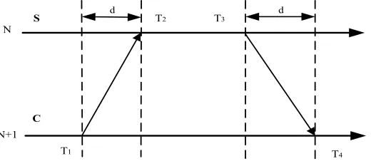
The N+l layer node C initiates the synchronization request information. This in-formation will carry the local transmission time Ti. The N layer node S receives the request information, records the local time T2, and carries the local transmission time of the Ti, T2 and response information T3. The node C receives this information, records the receiving time T4, so that the node C can calculate the time deviation of the S equal to [(T2-Ti) - (T4-T3)]/2. The node C then synchronizes time to S accord-ing to this time deviation. The synchronization process of the nodes of two adjacent levels is shown in Figure 2.

d d

N

N+1

S

C

T2

T1

T3

T4

Fig. 2. The synchronization process of the nodes of two adjacent levels

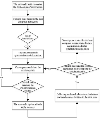
After the synchronization is completed, the aggregation node closes its own timer and reports the state of each node to the upper computer, and then goes back to the waiting state again. When the timer counts to 100 milliseconds, the two acquisition nodes will turn off the timer used in synchronization, open the timer used for acquisi-tion, and start the synchronous acquisition of 10 seconds with the sampling frequency of 8kHz. The flow chart of the synchronization process is shown in Figure 3.

The sink node waits to receive the host computer's instruction

The sink node receives the host computer instruction

Judge instructions

The sink node sends synchronization information

Convergence node into the receiving state

The sink node receives the synchronization

request

The sink node replies with the reply message

Collecting nodes calculates time deviations and synchronizes the time to the sink node

The sink node and the second acquisition node complete the

synchronization Convergence nodes like the host

computer to send status frames, acquisition nodes for synchronous acquisition OXOO

Yes No

No

3.3 Hardware design of sound acquisition node

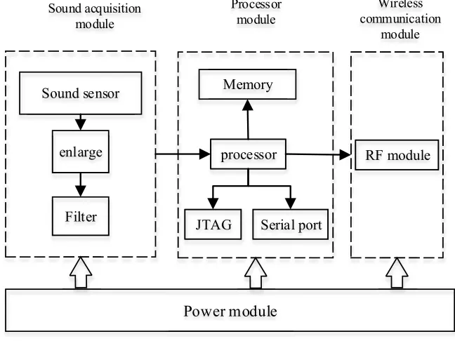
The acquisition and wireless transmission of sound signals is the main function of the sound acquisition node. It includes four modules: power supply, sound acquisi-tion, processor and wireless communication. The overall structure of the sound acqui-sition node is shown in Figure 4.

Sound sensor

processor Memory

JTAG Serial port

enlarge

Filter

RF module

Power module

Sound acquisition module

Processor

module communication Wireless module

Fig. 4. The overall structure of the sound acquisition node

As shown in Figure 4, the power supply module is responsible for power supply to the other three modules. The sound sensor in the sound acquisition module can detect the sound signal. It can convert the sound signal into an electrical signal and then be amplified and filtered. Finally, the A/D acquisition channel is connected to the pro-cessor. The processor converts the analog / number of the signal and stores the col-lected data into the expanded memory. According to the scheduling of the aggregation node, the processor will send out the data through the RF (radio frequency) module. The whole node uses JTAG to connect the door to download and debug the program. The serial port is used to print some program running status.

3.4 Application of fault source positioning

neces-sary to measure the distance at first. Many algorithms are based on the propagation time of the sound to get the distance of the sound. When the sound signal is transmit-ted to the beacon node, the sound signal is detectransmit-ted well and the arrival time of the sound is recorded. Precise time synchronization between nodes can be used as a refer-ence for subsequent parameter measurement. For the sound detection system, the sound acquisition module and the transplanted TPSN time synchronization algorithm have solved this key problem well.

In order to verify the application prospect of the system in the direction of sound source positioning, it is also a key point to select the appropriate location algorithm. The comparison and application analysis of the location algorithm will be introduced in the following.

At present, most of the location algorithms in wireless sensor networks include two steps. The first is the measurement of the distance (or angle), and then the location is calculated using these measurements. The methods of measuring distance (or angle) include RSSI, AOA, TOA, and TDOA. The main methods of location calculation are trilateration survey, triangulation and maximum likelihood estimate. Through the comparison of these location algorithms, it is concluded that in the four distance (or angle) measurement methods, the received signal strength indication (RSSI) algo-rithm is greatly influenced by environment and other factors, and the location accura-cy is relatively low. The signal arrival angle (AOA) algorithm is higher in hardware cost, maintenance cost and power consumption. It has a great load on the processor. The basic idea of the signal arrival time (TOA) and the signal arrival time difference (TDOA) algorithm are similar. The precision of the positioning is high. In the three location calculation methods, the triangulation method is used with the AOA algo-rithm. The maximum likelihood estimation method is obviously higher than the trilat-eration survey.

initialization

PC software waiting for user operation

Judgment button

PC software issued synchronization instructions

Synchronization between sink node and sink node

PC software waiting for user operation

PC software issued by the time instruction Judgment button Exit the program

Press the synchronization acquisition button

Yes Press the exit button

Press other button

The sink node sends the status of each node to the host computer

PC software to receive the status of each node and display

The sink node controls the buzzer to sound

Each node receives the acoustic signal and records the arrival time

Press to get the time button

Judgment button The aggregation node schedules

the collection node return time The sink node summarizes the signal arrival time and sends it Host computer to receive and

calculate the distance Three-way measurement of

positioning PC software waiting for the user

Draw and display the positioning result

!"#$$%&'#%$()*'"+)+,$ %-*.,/$/&/+)%0,&&+)

!"#$$%&'#%+&'#" %0,&&+)

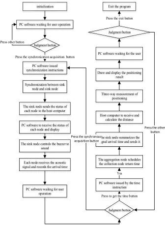
Fig. 5. The process of system positioning application software

After the initialization is completed, the host computer software enters the state of "waiting for the user to operate". Only when the "Simultaneous Acquisition" button on the software interface is pressed, the host software will exit the waiting state and send the synchronization command in the form of UDP message. This command is still "0x00".

When the sink node receives this command, it will perform TPSN time synchroni-zation with the two sound collection nodes. When the synchronisynchroni-zation process is completed, it reports itself and the status of the two acquisition nodes. This status is sent to the host computer through UDP packets. The first 3 bytes of the packet are valid. If all three nodes are connected properly, all three bytes are "0x37". According to the received status message, the PC software will display the status of several nodes on the interface. Under normal circumstances, the status of all three nodes should be displayed as Connected.

After the sink node sends the status message, the two sound collection nodes auto-matically enter the signal acquisition status. The time synchronization is completed. The synchronization process generally takes tens of milliseconds. Therefore, when the system is designed, after 100 milliseconds, the sink node will control the buzzer con-nected to I / O port to emit a sound signal.

Once the amplitude of the sound signal collected by each node is greater than the set threshold, the time of arrival of the signal and the arrival time of the signal are recorded.

After receiving the status message, the host software enters the state of "waiting for user operation". If the user presses the "synchronous acquisition" button, the host software will resend the synchronization command to schedule the convergence node to synchronize and sound.

If the user presses the "Get Time" button, the PC software will issue the instruction "OxOA". After receiving this instruction, the sink node sends "0x01" and "0x02" to the sink node 1 and the sink node 2, respectively. Two nodes record the signal arrival time. The aggregation node will summarize this time and send it to the host computer in the form of UDP packets. The first 6 bytes of this message are valid. Every 2 bytes is a unit. They represent the signal arrival time recorded by the sink node, the sound collection node 1, and the sound collection node 2, respectively.

PC software receives the time message for analysis. According to the agreement, three-time information is removed. Each arrival time minus 100 milliseconds, it is multiplied by the propagation speed of the acoustic signal to calculate the distance from the sound source point to each node. The formula of the trilateration survey is applied to get the data of the three intersection points. The center of gravity of the triangle is chosen to get the final coordinate of the sound source point. It is displayed on the host computer interface.

4

Result Analysis and Discussion

In the sound source localization experiment, the sound source is a buzzer con-trolled by the I/O port of the converging node. The buzzer is silent / sound based on the high / low level of the output of the I/O port. In the test, three beacon nodes are arranged in coordinates (0, 50), (-70, 0), and (70, 0) in the plane right angle nate system. The source point is placed in a position of (0, 20) (the units of all coordi-nates are centimeters). A total of five tests were carried out. The experimental data of the test are shown in Table 1.

Table 1. Experimental data of sound source localization test

cl c2 c3 x y

1 35 87 97 -5.1387 34.1167

2 33 89 74 7.708 26.6412

3 34 98 75 11.7901 30.8671

4 44 87 73 7.2549 17.9456

5 33 87 72 2.5705 28.7364

The average value of the measured source point coordinates is as follows:

6614

.

27

5

1

8370

.

4

5

1

=

=

=

=

!

!

y

y

x

x

The maximum error between the transverse and the actual coordinates measured by the source point is 11.7901. The average error is 4.8370. The maximum error between the measured and the actual coordinates is 14.1167. The average error is 7.6614. The reasons for the error are the environmental factors, the reflection and diffraction of the sound signals in the room. The time synchronization has error, which leads to the error of the sound signal propagation time calculated by each node. In the measure-ment of sound source positioning, the signal waveform of the test sound source and the experimental data of the positioning test are given. The error of the location of the data display system is small.

5

Conclusions

realized in the system and the hardware design of the sound detection system was introduced in detail. The application of sound detection system in the field of sound source localization was explored and the existing location algorithm was studied. The TOA and trilateration survey were also applied to the simple reformed system. Final-ly, the positioning test was carried out and the application of the sound detection sys-tem was tested. And the following results were obtained:

Firstly, after the sound detection system was introduced in detail, it was proved that the positioning error of the system is small.

Secondly, wireless sensor networks have the prospect of application in the field of sound source positioning.

At last, the error of the location of sound source in the data display system is small.

6

Acknowledgement

This paper is supported by the Science and technology project of Chongqing Mu-nicipal Education Committee: research and development of audio signal detection and troubleshooting system applied to radio broadcasting automatic broadcasting system (KJ1503901).

7

Reference

[1]Azharuddin, M., & Jana, P. K. A distributed algorithm for energy efficient and fault toler-ant routing in wireless sensor networks. Wireless Networks, 2015 _{vol. 21, pp. 251-267.}

https://doi.org/10.1007/s11276-014-0782-2

[2]Ahmed, A. A. A comparative study of qos performance for location based and corona based real-time routing protocol in mobile wireless sensor networks. Wireless Networks, 2015, vol. 21, pp. 1015-1031. https://doi.org/10.1007/s11276-014-0834-7

[3]Kariman-Khorasani, M., & Pourmina, M. A. Maximum lifetime routing problem in asyn-chronous duty-cycled wireless sensor networks. Wireless Networks, 2015, vol. 21, pp. 2501-2517. https://doi.org/10.1007/s11276-015-0931-2

[4]Nordio, A., Tarable, A., Dabbene, F., & Tempo, R.Sensor selection and precoding strate-gies for wireless sensor networks. IEEE Transactions on Signal Processing, 2015, vol. 6, pp. 4411-4421. https://doi.org/10.1109/TSP.2015.2439239

[5]Nevat, I., Peters, G. W., Septier, F., & Matsui, T. Estimation of spatially correlated random fields in heterogeneous wireless sensor networks. IEEE Transactions on Signal Processing, 2015, vol. 63, pp. 2597-2609. https://doi.org/10.1109/TSP.2015.2412917

[6]Platachaves, J., Bahari, M. H., Moonen, M., & Bertrand, A. Unsupervised diffusion-based lms for node-specific parameter estimation over wireless sensor networks. IEEE Transac-tions on Signal Processing, 2015, vol. 63, pp. 3448-3460. https://doi.org/10.1109/TSP.2015.2423256

[7]Schlupkothen, S., Dartmann, G., & Ascheid, G. A novel low-complexity numerical locali-zation method for dynamic wireless sensor networks. IEEE Transactions on Signal Pro-cessing, 2015, vol. 63, pp. 4102-4114. https://doi.org/10.1109/TSP.2015.2422685

[9]Ye, M., Wang, Y., Dai, C., & Wang, X. A hybrid genetic algorithm for the minimum ex-posure path problem of wireless sensor networks based on a numerical functional extreme model. IEEE Transactions on Vehicular Technology, 2016, vol. 65, pp. 8644-8657. https://doi.org/10.1109/TVT.2015.2508504

[10]Zhou, B., Chen, Q., & Xiao, P. The error propagation analysis of the received signal strength-based simultaneous localization and tracking in wireless sensor networks. IEEE Transactions on Information Theory, 2017, vol. 99, pp. 1-1. https://doi.org/10.1109/TIT.20 17.2693180

8

Authors

Min Shen and Zhiling Tang are with the Chongqing Technology and Business In-stitute, Chongqing, China.