Characteristics of a loop of evidence that affect detection and estimation of inconsistency: a simulation study

R E S E A R C H A R T I C L E

Open Access

Characteristics of a loop of evidence that affect

detection and estimation of inconsistency: a

simulation study

Areti Angeliki Veroniki

, Dimitris Mavridis

, Julian PT Higgins

and Georgia Salanti

Abstract

Background:The assumption of consistency, defined as agreement between direct and indirect sources of evidence, underlies the increasingly popular method of network meta-analysis. This assumption is often evaluated by statistically testing for a difference between direct and indirect estimates within each loop of evidence. However, the test is believed to be underpowered. We aim to evaluate its properties when applied to a loop typically found in published networks.

Methods:In a simulation study we estimate type I error, power and coverage probability of the inconsistency test for dichotomous outcomes using realistic scenarios informed by previous empirical studies. We evaluate test properties in the presence or absence of heterogeneity, using different estimators of heterogeneity and by employing different methods for inference about pairwise summary effects (Knapp-Hartung and inverse variance methods).

Results:As expected, power is positively associated with sample size and frequency of the outcome and negatively associated with the presence of heterogeneity. Type I error converges to the nominal level as the total number of individuals in the loop increases. Coverage is close to the nominal level in most cases. Different estimation methods for heterogeneity do not greatly impact on test performance, but different methods to derive the variances of the direct estimates impact on inconsistency inference. The Knapp-Hartung method is more powerful, especially in the absence of heterogeneity, but exhibits larger type I error. The power for a‘typical’loop (comprising of 8 trials and about 2000 participants) to detect a 35% relative change between direct and indirect estimation of the odds ratio was 14% for inverse variance and 21% for Knapp-Hartung methods (with type I error 5% in the former and 11% in the latter).

Conclusions:The study gives insight into the conditions under which the statistical test can detect important inconsistency in a loop of evidence. Although different methods to estimate the uncertainty of the mean effect may improve the test performance, this study suggests that the test has low power for the‘typical’loop.

Investigators should interpret results very carefully and always consider the comparability of the studies in terms of potential effect modifiers.

Keywords:Mixed treatment comparison, Multiple interventions, Coherence, Consistency, Simulation study, Bias

* Correspondence:[email protected] 1

Department of Hygiene and Epidemiology, University of Ioannina School of Medicine, University Campus, Ioannina 45110, Greece

Full list of author information is available at the end of the article

Background

The validity of results from network meta-analysis de-pends on the plausibility of the transitivity assumption; that is the comparability of studies informing the treat-ment comparisons with respect to the distribution of ef-fect modifiers [1-3]. Lack of transitivity in a network can create statistical disagreement between direct and vari-ous sources of indirect evidence, often termed inconsist-ency [4]. Statistical evaluation of consistinconsist-ency is possible only when there are‘closed loops of evidence’in the net-work. The recent increase in applications of network meta-analysis has emphasised the need for methods to evaluate consistency and has motivated the development of statistical models [5-7] and methods [8-11].

Empirical evidence suggests that the prevalence of statis-tically significant loop inconsistency ranges from 2% to 17% [12-14]. However, little is known about factors that impact on the detection of inconsistency. As expected, the power to detect inconsistency is positively associated with the number and size of trials, and both power and type I error increase when a fixed-effect model is assumed [15]. It has been argued that the presence and magnitude of heterogeneity (within comparison variability) in a loop of evidence can impact on inferences made about inconsist-ency and empirical evidence has confirmed these claims by showing that different estimators of the heterogeneity variance are likely to have a considerable impact [14]. Fi-nally, previous studies showed that inconsistency occurs more frequently in loops where one of the comparisons is informed only by one trial [14,16,17].

Although there are indications that the presence, mag-nitude and estimation method of heterogeneity might influence the detection of inconsistency, this association has not been studied extensively. For instance, the im-pact of two alternative methods to express uncertainty about the pairwise summary effects (inverse variance and Knapp-Hartung method [18,19]) remains unclear. It has been shown that the Knapp-Hartung method out-performs inverse variance in coverage for the summary effect and that it is insensitive to the estimator of the heterogeneity used [20,21]. We anticipate that differ-ences in the properties of the two methods will impact on the estimation of inconsistency.

The aim of this paper is to explore factors that affect the detection of inconsistency in a three-treatment net-work for a dichotomous outcome. The factors that we explore are associated with the amount of data available in the loop (such as number, size and distribution of tri-als across comparisons, frequency of events), the hetero-geneity variance in the pairwise comparisons (presence or absence and estimation method) and the method for inference about pairwise summary effects (inverse vari-ance or Knapp-Hartung). We consider only log-odds ra-tio (LOR) as the effect size of interest. We conduct a

simulation study considering realistic scenarios including only two-arm trials and we estimate type I error, power and coverage probability for the test of consistency. The simulation scenarios are informed by two previous em-pirical studies; a large collection of 303 loops from pub-lished networks of interventions [14] and a study about the empirical distribution of heterogeneity on dichotom-ous outcomes [22].

Methods

The inconsistency test

Consider a simple scenario with three competing treat-ments A, B and C and that there are trials that compare directly all three possible pairs of treatments. Evaluation of inconsistency in a triangular network requires first the estimation of three direct summary effects for each pairwise comparison. We denote the effect sizes (i.e. LORs) for the three pairs of treatments as^μDIR

AB;μ^DIRAC and ^

μDIR

BC with variances^vDIRAB;v^DIRAC and ^vDIRBC respectively. The superscript denotes the source of evidence (‘DIR’for direct here or‘IND’indirect later) and the subscript denotes the treatment comparison. For any given comparison (e.g. BC) we estimate the indirect mean treatment effect,μ^IND

BC , as a simple contrast of two direct estimates involving the third treatment, and we compare it with the corresponding dir-ect estimate^μDIR

BC.

The inconsistency factor (IF) for the loop ABC is esti-mated as

IF

∧

ABC¼^μDIRBC−μ^INDBC ¼μ^DIRBC−^μDIRAC þμ^DIRAB

with variance

^

vIFABC¼^v

DIR

BC þv^INDBC ¼^vDIRBC þ^vDIRAC þ^vDIRAB ð1Þ

The direction of the estimated IF is irrelevant to the evaluation of inconsistency and only the magnitude of its absolute value is of interest. The subscript in IF∧_ABC refers to the loop in which inconsistency is estimated.

Under the null hypothesis of consistency (H0: IF = 0) a

z-test is calculated

z¼ IF

∧

ABC

ffiffiffiffiffiffiffiffiffiffiffi

^ vIFABC

p _eN 0;ð 1Þ;

with a critical region |z|≥ z_a/2. In the present study we

selecta= 0.05.

Estimation of variance

Equation (1) suggests that the method used to estimate the variance of the direct treatment effects vDIR_AB;vDIR_AC and vDIR

can impact on the estimation of vIFABC. The first method

is the usual inverse-variance method and the second method is an alternative approach proposed by Knapp and Hartung [19].

In a pairwise meta-analysis we either assume that trials estimate a single underlying effect size (fixed-effect model) or that the study-specific underlying effect sizes are differ-ent but drawn from the same distribution (random effects model) with heterogeneityτ2. Under the latter scenario, it is common to assume that heterogeneity is the same for all comparisons being made, i.e. τ2

AB¼τ2AC¼τ2BC¼τ2. We adopt this assumption throughout the paper and we esti-mateτ2using the DerSimonian and Laird estimator [23].

In the inverse variance approach, the direct variances are simple functions of the sampling variances of the in-dividual trials and the heterogeneity varianceτ2. Suppose that KAB, KACand KBCtrials inform the AB, AC and BC

comparisons respectively. If the sampling variances were the same for all trials (σ2), the inverse variance estimator of the inconsistency variance would be

^

vIFABC¼^σ

2 1

KAB þ 1

KAC þ 1

KBC

þ3^τ2: ð2Þ

Consequently,^vIFABC depends on the heterogeneity and

decreases with the number and precision of the included trials.

An alternative approach to estimate each direct variance, and consequently vIFABC , is the approach proposed by

Knapp and Hartung [19]. They derive the variancev^DIR AB as the ratio of a generalised Q statistic divided by the product of the degrees of freedom (KAB− 1) and the sum of the

random-effects study weights [24]. It has been shown that the performance of this method is not influenced by the choice of the heterogeneity estimator [19,21,25,26].

In summary, we estimate the variances of the direct pairwise summary effects by employing two different strat-egies: the inverse variance method using DerSimonian and Laird estimator (IVDL) and the Knapp-Hartung method with the DerSimonian and Laird estimator (KHDL). When a comparison is addressed by a single trial (so that the loop includes 3 trials in total) estimation of heterogeneity is impossible. In these cases we use the fixed-effect model (by settingτ2to be zero) and consequently both IVDL and KHDL methods would yield exactly the same results.

Simulation study

Empirical evidence to inform simulation scenarios

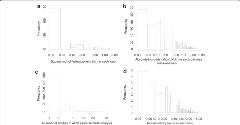
To inform the simulation scenarios we use a large collec-tion of complex networks of intervencollec-tions [14]. Figure 1 summarises some of the attributes of 303 loops from 40 published networks with dichotomous outcomes ana-lysed using the LOR scale. The majority of the pairwise meta-analyses (93%) included fewer than ten trials. The

Frequency

d

Inconsistency factor in each loop

Frequency

1 2 5 10 20 50

0

100

200

300

400

500

c

Number of studies in each pairwise meta-analysis

Frequency

a

Square root of heterogeneity ( ) in each loop

Frequency

b

Absolute log-odds ratio ( ) in each pairwise meta-analysis

0.05 0.10 0.20 0.50 1.00 2.00

0

2

0

4

0

6

0

8

0

100

120

0.00 3.00

0.05 0.10 0.20 0.50 1.00 2.00 5.00

0

5

10

15

20

25

30

35

0.00 0.05 0.10 0.20 0.50 1.00 2.00

05

0

100

150

0.00

median |LOR| is 0.32 with interquartile range (IQR) (0.13, 0.75). In 91% of the loops the common within-loop hetero-geneity using the DerSimonian and Laird estimator is less than 0.5 and it is estimated at zero (when rounded to the second decimal) in 51% of the loops. The median IF is 0.36 with IQR (0.15, 0.80). The median number of trials per loop is 8 IQR (6, 14) and the median loop sample size is 2256 IQR (1026, 18890); the respective median number of trials and sample size per comparison are 2 IQR (1, 4) and 706 IQR (255, 2997). Most networks had a subjective primary outcome (43%), whereas 35% and 22% of the networks had reasonably objective outcomes (e.g. cause-specific mortal-ity, major morbidity event) and all-cause mortality out-comes respectively. The majority of the networks (63%) compared pharmacological interventions versus placebo. In the case of such a comparison type and subjective out-come, Turner et al. suggest that the distribution of the heterogeneity is reasonably approximated by a log-normal τ2

~ LN(−2.13, 1.582), with median τ2 = 0.12 and IQR (0.03, 0.34) [22]. Our empirical data seem to match the predictive distribution suggested by Turner et al. [22] (τ2

~ LN(−2.13, 1.582)), though more data are needed since we have only 55 common within-loop heterogeneities estimated in networks with pharmacological interven-tions versus placebo comparison type and subjective outcome.

Simulation scenarios

We use subscripts k1, k2and k3to refer to the three

com-parisons AB, AC and BC respectively, so that k1= 1,…,

KAB, k2= 1,…, KACand k3= 1,…, KBC, where KAB, KAC,

KBC represent the number of trials included in AB, AC

and BC comparisons respectively. We examine both bal-anced direct comparisons, i.e. all comparisons include the same number of trials KAB = KAC = KBC= K = 1, …, 7,

and imbalanced direct comparisons, i.e. each comparison is informed by a different number of trials with KAB = 1,

KAC= 4, KBC= 7. Both balanced and imbalanced scenarios

were selected, informed by the empirical data. In particu-lar, the imbalanced scenario included a comparison with a single trial, because the majority (196 out of 303) of ob-served loops had this characteristic. We then set the sec-ond comparison to include a large number of trials (7 trials) and for the third comparison we selected the median between the two extremes (4 trials). We restrict our ana-lysis to dichotomous outcome data measured using odds-ratio (OR) due to its mathematical properties [27-29]. Based on the results from the empirical study [14], we as-sume ORAB= 1/exp(0.32) = 0.73 and ORAC= 1 the

rela-tive treatment effects for AB and AC respecrela-tively. We compute the OR for the BC comparison as

ORBC¼ exp log ORf ð ACÞ−log ORð ABÞ þIFABCg:

We select values IFABC = {0, 0.3, 0.45, 0.6, 1} to cover a

range of plausible values for inconsistency as suggested by empirical data (Figure 1d). We consider two different distri-butions for heterogeneity that pertain to a subjective out-come (the most frequently reported outout-come in our data) and all-cause mortality for comparisons between pharma-cological interventions and placebo; according to [22] these are τ2~ LN(−2.13, 1.582) and τ2~ LN(−4.06, 1.452) (me-dianτ2= 0.02 with (IQR 0.01, 0.04)).

For each combination of OR, IFABC, andτ2we simulate

the trial-specific underlying relative treatment effects from a normal distribution as

LORAB;k1eN LORAB; τ

2

ð Þ , LORAC;k2eN LORAC; τ

2

ð Þ

and LORBC;k3eN LORBC; τ

2

ð Þ:

Then, we generate arm-level data for each trial k1, k2

and k3. Without loss of generality we describe how to

obtain arm-level data for an AB trial. We assume equal sample sizes across arms, that is nA;k1 ¼nB;k1¼n . The

observed IQR for arm sample size in our empirical data is 51 to 270, and to represent moderate and large studies we generated studies with n ~ U(50, 150) and n ~ U (150, 300). We also considered n ~ U(20, 50) to generate data for very small studies. The number of events per arm, denoted with rA;k1 and rB;k1 are drawn from two

binomial distributions rA;k1eBðnA;k1; pA;k1Þ and rB;k1eB

ðnB;k1; pB;k1Þ where pA;k1 and pB;k1 are the

probabil-ities of the outcome in each trial arm. To define these probabilities we make assumptions about the average risk (AR) of the outcome in the trial assuming both frequent and rare events. To simulate from frequent event rates we draw from a uniform distribution ARAB;k1eU 0:25;ð 0:75Þ

and for rare events ARAB;k1eU 0:05;ð 0:15Þ:

Then the event probabilities in the arms are obtained as the solution to the equations

ARAB;k1 ¼

p_A;k1þp_B;k1 2

LORAB;k1¼ log

pA;k1 1−pB;k1

p_B;k1 1−p_A;k1

0 @

1 A

For frequent events and assuming no heterogeneity, the expected mean variance of LOR ranges from 0.04 to 0.25 depending on sample size. Variances for LOR for rare events range from 0.10 to 0.69.

We then calculate the sample LOR and its variance as

LOR_AB;k1¼ log rA;k1 nB;k1−rB;k1

rB;k1 nA;k1−rA;k1

v_AB;k1¼ 1 rA;k1

þ 1

nA;k1−rA;k1

þ 1 rB;k1

þ 1

nB;k1−rB;k1

If the simulated number of events in one of the study arms is zero, we add 0.5 to the cells of the 2 × 2 table. We repeat this process for all KAB trials and then we

perform a random-effects meta-analysis to obtain the summary effect size μ^DIR

AB . We follow the same process for comparisons AC and BC and then we estimate the inconsistency factor. Table 1 presents a summary of the simulation scenarios considered.

For each scenario we analyse 1000 simulated triangular networks. Assuming a 5% significance level, we estimate the power of the test when true inconsistency is present (P(|z|≥ 1.96|IF≠0) and type I error when the null hy-pothesis is true (P(|z| ≥ 1.96|IF = 0). We compute the coverage probability for the confidence interval (CI) of inconsistency, which is the probability that the estimated interval for IF includes its true value. We carry out the

simulations in the freely available software R 2.15.2 [30] using the self-programmed sims.fun function, which we have made available online (http://www.mtm.uoi.gr/index. php/material-from-publications-software-and-protocols).

In addition to the scenarios described above we also consider an extra scenario representing the‘typical’loop; that is a loop with the characteristics most commonly encountered in our collection of 303 loops. We specified this such that one comparison was informed by a single trial and the median number of studies per loop was 8, in line with the empirical evidence. The median loop sample size is 2300 (i.e. average trial arm size 144) [14]. Consequently, a loop with KAB = 1, KAC = 4, KBC = 3,

and n ~ U(120, 160) can be considered to be an‘average sized loop’.

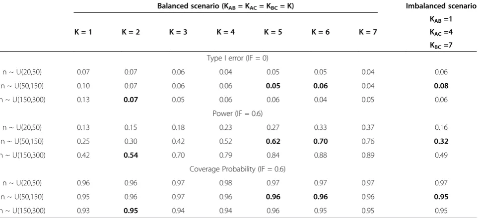
Results Type I error

Figure 2 and Additional file 1: Figure S1 display the esti-mated type I error for equal and different numbers of trials across comparisons. In general, type I error is close to the nominal level for IVDL, but larger than 5% for many scenarios analysed with KHDL. The KHDL method generally yields smaller variances for IF, leading to larger type I errors (average type I error across all narios for IVDL: 0.07, average type I error across all sce-narios for KHDL: 0.10, see also Figure 2a and b). Type I error converges to the nominal level more rapidly when τ2

= 0 for both IVDL and KHDL methods. The overall type I error approaches the nominal level as the number of trials increases for the same trial size. For example, for frequent events type I error reaches on average the nominal level when K = 5 for small sample sizes, and K = 4 for moderate and large sample sizes. In Table 2 we provide the type I error values for various simulation scenarios. When the total number of individuals in-cluded in the network ranges from 2400 to 3000 (i.e. close to the empirically estimated median loop size) type I error lies between 0.06 and 0.08. Type I error deviates from 5% considerably when an equal and small number of trials is considered across comparisons for all trial sizes (see Figure 2a ,b and Table 2).

For rare events, type I error departs from 5% more than it does for frequent events (Figure 2). Type I error is lower than its nominal level in most cases for IVDL especially whenτ2= 0, probably due to overestimation of τ2

. The KHDL method results again in considerably lar-ger type I errors, which is probably due to the small vari-ances of the mean treatment effects (average type I error across all scenarios for IVDL: 0.05, average type I error across all scenarios for KHDL: 0.08, see Figure 2c and d). Type I error is closer to the nominal level for IVDL whenτ2≠0 for all sample sizes. All methods tend to im-prove their performance with increasing total number of Table 1 Summary of the simulation scenarios

Number of studies

Balanced direct

comparisons KAB= KAC= KBC= 1,…, 7

Imbalanced direct comparisons

KAB= 1, KAC= 4, KBC= 7 (and KAB= 1, KAC= 4, KBC= 3 for the typical loop)

Treatment effects

Comparison AB ORAB= 0.73

Comparison AC ORAC= 1

Comparison BC ORBC= exp{log(ORAC)₋log(ORAB) + IFABC} Inconsistency in the network

Inconsistency Factor IFABC= {0, 0.3, 0.45, 0.6, 1}

Heterogeneity in the network

Subjective outcome τ2_{~ LN(−2.13, 1.58}2₎ All-cause mortality

outcome τ

2_{~ LN(−4.06, 1.45}2₎

Trial arm size nA;k1¼nB;k1¼n

Small n ~ U(20, 50)

Moderate n ~ U(50, 150)

Large n ~ U(150, 300) (and n ~ U(120, 160) for the_{typical loop)}

Frequency of events

Average risk for

frequent events ARAB;k1eU 0ð:25;0:75Þ

Average risk for rare

events ARAB;k1eU 0ð:05;0:15Þ

Approaches to estimate the variances of the direct pairwise summary effects

Inverse variance method

Type I error

Total number of individuals in the loop

Balanced Scenario ( )

b frequent events with

200 500 1000 2000 5000 10000

0.0

0

.1

0.2

0

.3

0.4

c rare events with

200 500 1000 2000 5000 10000

0.0

0.1

0.2

0.3

0.4

d rare events with

200 500 1000 2000 5000 10000

0.0

0.1

0.2

0.3

0.4

a frequent events with

200 500 1000 2000 5000 10000

0.0

0

.1

0.2

0.3

0

.4

IVDL KHDL

Small sample size

Moderate sample size Large sample size

1

Figure 2Type I error by sample sizes, frequency of events and loop sample size.We assumeequalnumber of trials per comparison (KAB= KAC= KBC= K = 1,…, 7) in the presence (τ2≠0) and absence (τ2= 0) of heterogeneity. Circled points correspond to loops with K = 1 for which a fixed-effects model is employed. The region within the horizontal dotted lines defines the confidence interval for the 5% nominal level. IVDL: inverse variance method using the DerSimonian and Laird estimator, KHDL: Knapp-Hartung method with the DerSimonian and

Laird estimator.

Table 2 Type I error, power and coverage probability by sample size and number of trials

Balanced scenario (KAB= KAC= KBC= K) Imbalanced scenario

K = 1 K = 2 K = 3 K = 4 K = 5 K = 6 K = 7

KAB=1

KAC=4

KBC=7

Type I error (IF = 0)

n ~ U(20,50) 0.07 0.07 0.06 0.04 0.05 0.05 0.04 0.06

n ~ U(50,150) 0.10 0.07 0.06 0.06 0.05 0.06 0.04 0.08

n ~ U(150,300) 0.13 0.07 0.05 0.06 0.06 0.04 0.05 0.06

Power (IF = 0.6)

n ~ U(20,50) 0.13 0.15 0.18 0.23 0.27 0.33 0.37 0.16

n ~ U(50,150) 0.25 0.30 0.42 0.52 0.62 0.70 0.76 0.32

n ~ U(150,300) 0.42 0.54 0.70 0.79 0.84 0.88 0.89 0.49

Coverage Probability (IF = 0.6)

n ~ U(20,50) 0.96 0.96 0.97 0.98 0.97 0.97 0.97 0.97

n ~ U(50,150) 0.95 0.96 0.97 0.96 0.96 0.96 0.96 0.95

n ~ U(150,300) 0.93 0.95 0.94 0.94 0.96 0.95 0.95 0.95

trials included in the entire network (Figure 2 and Additional file 1: Figure S1).

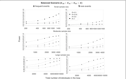
Statistical power

Figure 3 and Additional file 2: Figure S2 present the power for IF = {0.3, 0.45, 0.6, 1} for both frequent and rare events when equal (Figure 3) and different (Additional file 2: Figure S2) numbers of trials are included in compari-sons. As expected, the overall power increases both with number of trials included in the loop and with the trial size. Power increases when the trials included in a loop have comparable sample sizes. Results are aggregated over all estimation methods for heterogeneity and the different methods to estimate the variance of the direct summary effects. In Table 2 we provide the power values for various simulation scenarios when IF = 0.6 and fre-quent events are considered. When the total number of individuals included in the network ranges from 2400 to 3000, power ranges between 0.54 and 0.70 when an equal number of trials is assumed across comparisons but drops to 0.32 when each comparison has a different number of trials. As can be seen in equation (2), the distribution of

trials across comparisons affects the estimation of incon-sistency variance. This has an impact on power and the test is more powerful when trials are distributed uniformly across comparisons. Comparing, for example, the power of the test for the balanced scenario KAB = 4, KAC = 4,

KBC= 4 and the imbalanced scenario KAB= 1, KAC= 4,

KBC= 7 (each with 12 trials in the loop), power is higher

when the distribution of trials is balanced across compari-sons (ranges from 0.23 to 0.79) rather than imbalanced (ranges from 0.16 to 0.49) (see Table 2). The comparison of frequent (Figure 3a) and rare (Figure 3b) events indi-cates that power is larger for frequent events (average power across all scenarios for frequent events: 0.44, aver-age power across all scenarios for rare events: 0.25). Rare events are associated with larger uncertainty for the direct mean treatment effects and thus the chances of identifying potentially important inconsistency decrease. It should be noted that the first summary result of each power curve pertains to the case where there is only one trial per com-parison and heterogeneity is set to be zero. This has an impact on monotonicity especially when IF is low and trial size is large.

a frequent events

Power

Balanced Scenario ( )

Total number of individuals in the loop

b rare events

200 400 600 800 1000 1400

0.0

0.2

0.4

0.6

0.8

1.0

1000 2000 3000 4000

0.0

0.2

0.4

0.6

0.8

1.0

2000 4000 6000 800010000

0.0

0.2

0.4

0.6

0.8

1.0

Small sample size

Moderate sample size

Large sample size

200 400 600 80010001200

0.0

0.2

0.4

0.6

0.8

1.0

1400

1000 2000 3000 4000

0.0

0.2

0.4

0.6

0.8

1.0

2000 4000 6000 8000 10000

0.0

0.2

0.4

0.6

0.8

1.0

IF=0.3 IF=0.45 IF=0.6 IF=1

In Tables 3 and 4 we present the power for IVDL and KHDL methods. For frequent events the power to detect inconsistency does not vary significantly with the method used to estimate heterogeneity or to express uncertainty on the summary effects although the Knapp-Hartung method is marginally more powerful, especially in the absence of heterogeneity. This is because, in many cases, the Knapp-Hartung method estimates smaller inconsistency variances compared with the inverse variance method. The median inconsistency standard error is 0.33 (IQR 0.21, 0.50) for KHDL and 0.40 (IQR 0.27, 0.57) for IVDL. As expected, when there is no heterogeneity, there is less uncertainty as-sociated with each pairwise effect and the power to detect inconsistency increases for all IF values (Table 3).

The impact of heterogeneity is similar when the out-come is rare (average power across all IF values for KHDL: 0.24, average power across all IF values for IVDL: 0.21, see Table 3). Table 3 shows that the advantage of KHDL method when heterogeneity is zero becomes more pronounced for rare events (average power across all IF values for KHDL: 0.32, average power across all IF values for IVDL: 0.25, see Table 3).

Coverage probability and bias

We assess how often the 95% CI for inconsistency in-cludes the assumed IF value used to generate the data. We plot the coverage probability for the 95% CI of IF in Additional file 3: Figure S3. The coverage probability is close to the nominal level (95%) for most settings. Rare

events are associated with larger uncertainty and therefore provide slightly higher coverage than frequent events (average coverage across all scenarios for frequent events: 0.95, average coverage across all scenarios for rare events: 0.97). In Table 2 we provide the coverage values for vari-ous simulation scenarios when IF = 0.6. When the total number of individuals included in the network ranges from 2400 to 3000, coverage ranges from 0.95 to 0.96 (Table 2). Coverage does not change considerably when an equal or different number of trials is assumed across com-parisons (Additional file 4: Figure S4).

In Additional file 5: Figure S5 and Additional file 6: Figure S6 we present the average relative biasI^F−IF=IF for IF > 0. Relative bias decreases with the total number of individuals included in the network, the total number of tri-als, and the assumed IF value.

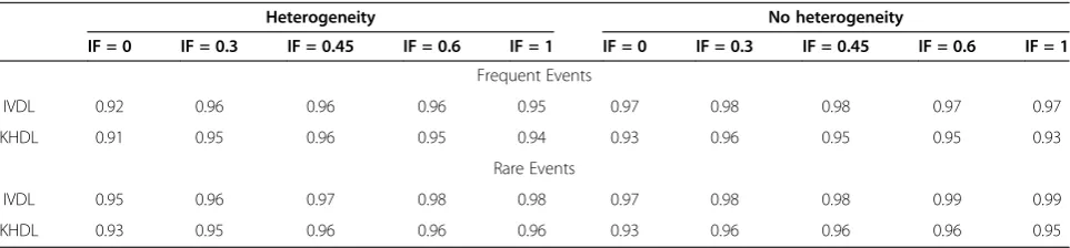
Tables 5 and 6 present the coverage probability for the 95% CI of IF using different methods to express un-certainty on the summary effects. The KHDL method reduces slightly the chances of including the true incon-sistency factor in the 95% CI of IF, especially when there is no heterogeneity, as the mean treatment effects be-come more precise.

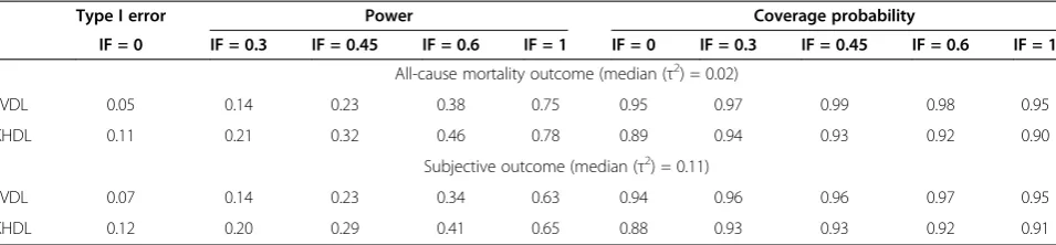
Characteristics of the inconsistency test in a‘typical’loop of evidence

The type I error in the ‘typical’ loop is 5% and 7% for subjective and all-cause mortality outcomes using IVDL Table 3 Power of the test for inconsistency aggregated over sample size and number of trials

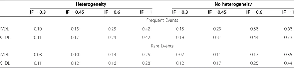
Heterogeneity No heterogeneity

IF = 0.3 IF = 0.45 IF = 0.6 IF = 1 IF = 0.3 IF = 0.45 IF = 0.6 IF = 1

Frequent Events

IVDL 0.17 0.26 0.36 0.59 0.20 0.38 0.52 0.77

KHDL 0.19 0.27 0.37 0.60 0.27 0.44 0.58 0.80

Rare Events

IVDL 0.10 0.15 0.21 0.38 0.09 0.16 0.25 0.49

KHDL 0.13 0.18 0.24 0.41 0.16 0.23 0.33 0.55

Results are presented forequalnumber of trials across comparisons. IF: inconsistency factor, IVDL: inverse variance method with the DerSimonian and Laird estimator, KHDL: the Knapp-Hartung method with the DerSimonian and Laird estimator.

Table 4 Power of the inconsistency test aggregated over sample size

Heterogeneity No heterogeneity

IF = 0.3 IF = 0.45 IF = 0.6 IF = 1 IF = 0.3 IF = 0.45 IF = 0.6 IF = 1

Frequent Events

IVDL 0.10 0.15 0.23 0.42 0.13 0.23 0.38 0.68

KHDL 0.11 0.17 0.24 0.42 0.19 0.31 0.44 0.73

Rare Events

IVDL 0.08 0.10 0.14 0.25 0.07 0.11 0.17 0.35

KHDL 0.11 0.12 0.16 0.28 0.12 0.17 0.25 0.44

and 11% and 12% using KHDL. The‘typical’loop of evi-dence with all-cause mortality outcome has considerably low power. The overall power ranges between 14% and 75% for IVDL and 21% to 78% for KHDL depending on the magnitude of inconsistency. For a subjective out-come that pertains to larger heterogeneity power de-creases to 14%-63% for IVDL and in 20% to 65% for KHDL. Coverage is close to the 95% nominal level (see Table 7).

Discussion

The increased use of network meta-analysis should be accompanied by caution when combining direct and in-direct evidence via careful assessment of the consistency assumption. Protocols of network meta-analyses should present methods for the evaluation of inconsistency and define strategies to be followed when inconsistency is present. Several methodologies have been outlined in the literature to test inconsistency [4-9]. In this study, we evaluate the properties of the z-test for detecting in-consistency comparing direct and indirect estimates in triangular networks generating 1000 loops for each sce-nario presented in Table 1. Although running more than 1000 simulations per scenario would have decreased the Monte Carlo error, we believe the main conclusions from our simulations are robust. Our scenarios are in-formed by previous large-scale empirical studies and hence are directly applicable [14,22]. We use a variety of scenarios that involve the most commonly used

meta-analytic tools for statistical inference regarding heterogen-eity and the uncertainty of the mean treatment effects. The main advantage of this work is that it sheds light on factors that might affect the detection of inconsistency and have not been examined in the past, such as the use of Knapp-Hartung variance for the direct summary effects. Our main findings are summarized below.

The assumption of consistency in network meta-analysis is often evaluated performing a z-test within each loop of evidence.

The inconsistency test has low power for the‘typical’ loop (comprising 8 trials and about 2000 partici-pants) found in published networks. This study suggests that the probability to detect inconsistency when present is between 14% and 21% depending on the estimation method.

Power is positively associated with sample size and frequency of the outcome, and negatively associated with the underlying extent of heterogeneity.

Using the Knapp-Hartung method to estimate uncertainty around meta-analytic effects is slightly more powerful than the inverse variance approach. Type I error converges to the nominal level as the

total number of individuals included in the loop increases while coverage is close to the nominal level for most studied scenarios.

We recommend that investigators a) employ a variety of methods to evaluate inconsistency, b)

Table 5 Coverage probability of the 95% confidence interval for the inconsistency factor (IF)

Heterogeneity No heterogeneity

IF = 0 IF = 0.3 IF = 0.45 IF = 0.6 IF = 1 IF = 0 IF = 0.3 IF = 0.45 IF = 0.6 IF = 1

Frequent Events

IVDL 0.90 0.94 0.94 0.94 0.93 0.96 0.98 0.97 0.97 0.97

KHDL 0.89 0.93 0.93 0.93 0.91 0.92 0.95 0.94 0.94 0.93

Rare Events

IVDL 0.93 0.96 0.96 0.97 0.96 0.97 0.98 0.99 0.98 0.96

KHDL 0.91 0.95 0.95 0.95 0.94 0.92 0.96 0.96 0.95 0.94

Results are aggregated over sample size and number of trials (assumedequalacross comparisons). IVDL: inverse variance method with the DerSimonian and Laird estimator, KHDL: Knapp-Hartung method with the DerSimonian and Laird estimator.

Table 6 Coverage probabilities of the 95% confidence interval for the inconsistency factor (IF)

Heterogeneity No heterogeneity

IF = 0 IF = 0.3 IF = 0.45 IF = 0.6 IF = 1 IF = 0 IF = 0.3 IF = 0.45 IF = 0.6 IF = 1

Frequent Events

IVDL 0.92 0.96 0.96 0.96 0.95 0.97 0.98 0.98 0.97 0.97

KHDL 0.91 0.95 0.96 0.95 0.94 0.93 0.96 0.95 0.95 0.93

Rare Events

IVDL 0.95 0.96 0.97 0.98 0.98 0.97 0.98 0.98 0.99 0.99

KHDL 0.93 0.95 0.96 0.96 0.96 0.93 0.96 0.96 0.96 0.95

interpret the magnitude of the estimated inconsis-tency factor and its confidence interval c) adopt a sceptical stance towards statistically non-significant test results unless the loop of evidence has many data d) always consider the comparability of the studies in terms of potential effect modifiers to infer about the possibility of inconsistency

Our simulation study shows that the inconsistency test has on average low power to detect inconsistency, in particular for rare outcomes (i.e. for IF = 0.3 and large trial sizes a rare outcome has event rate on average 0.10 IQR (0.07, 0.13)). Bruadbrn et al. [31] state that the IVDL method may be “unsuitable when there are few events” and that it should be avoided. In the absence of heterogeneity and for a large number and size of trials the overall power for inconsistency might be adequate. A previous simulation study [15] also found that differ-ent ways to evaluate inconsistency (e.g. Lu and Ades [6] model, node-splitting method [9]) have low power in particular under the random-effects models. Our study suggests that power is improved if the Knapp-Hartung method is used, especially in the absence of heterogen-eity, although the type I error increases as well. This is because the estimated uncertainty around inconsistency is small with Knapp-Hartung method. These findings agree with a previous simulation study, which showed that when heterogeneity is zero the Knapp-Hartung method yields a smaller variance for the mean treatment effects than the inverse variance method [21].

Several methods have been suggested to estimate het-erogeneity τ2 [32,33]. In the present study we also in-cluded the restricted maximum likelihood [34] and the empirical Bayes [35] estimators in conjunction with the inverse variance approach. Although the three estima-tors have different properties and performance in gen-eral, they have been showed to have comparable bias and mean squared error for estimating τ2 in the exam-ined simulation scenarios (relatively small number of tri-als for each pairwise meta-analysis (fewer than 7) and

median heterogeneityτ2= 0.12 are comparable [32]. Con-sequently type I error, power and coverage were found similar between the three methods (data not shown) and we present results only from IVDL and KHDL. This agrees with an empirical study that compared five different estimators for the heterogeneity and showed that varia-bility in the confidence intervals of the overall treatment effect was quite negligible across 920 Cochrane meta-analyses [36].

The inconsistency test, analogously to the heterogeneity test, has low power and we recommend that the point es-timate of inconsistency and its 95% confidence interval are used instead to draw inferences about the presence and magnitude of inconsistency. In cases where the test is underpowered, the confidence intervals would include zero, small and large inconsistency values and should be interpreted as lack of evidence for or against the presence of inconsistency. If a test must be used, one possibility is to use a cut-off p-value of 0.10, as has been suggested for the heterogeneity test in pairwise meta-analysis [37,38]. Empirical evidence showed that the observed disagree-ment between direct and indirect comparisons is 1 in 10 loops, so this cut-point might be a reasonable choice [14]. In complex networks, instead of using multiple underpow-ered z-test, global tests such as the design-by-treatment test can be used, although power properties of the latter are unknown.

Some limitations in our study need to be acknowledged. We do not account for the possible impact of multi-arm trials on inconsistency and we only reconsider triangular networks. Our previous empirical study showed that a large majority (85%) of published networks of interven-tions involve trials with multiple arms, and that out of the total 1173 trials included in all 40 networks 116 (10%) were multi-arm trials. Further simulation studies are there-fore needed to evaluate complex networks with multi-arm trials. In our simulation study we assume that all compari-sons in the network share the same amount of heterogen-eity. Turner et al. [22] showed that different amounts of heterogeneity can be expected for different outcomes or for Table 7 Type I error, power and coverage probability for the inconsistency test in a‘typical’loop of evidence

Type I error Power Coverage probability

IF = 0 IF = 0.3 IF = 0.45 IF = 0.6 IF = 1 IF = 0 IF = 0.3 IF = 0.45 IF = 0.6 IF = 1

All-cause mortality outcome (median (_τ2_{) = 0.02)}

IVDL 0.05 0.14 0.23 0.38 0.75 0.95 0.97 0.99 0.98 0.95

KHDL 0.11 0.21 0.32 0.46 0.78 0.89 0.94 0.93 0.92 0.90

Subjective outcome (median (_τ2_{) = 0.11)}

IVDL 0.07 0.14 0.23 0.34 0.63 0.94 0.96 0.96 0.97 0.95

KHDL 0.12 0.20 0.29 0.41 0.65 0.88 0.93 0.93 0.92 0.91

We assume a dichotomous frequent outcome, number of trials (K) per comparison KAB= 1, KAC= 4, KBC= 3 and the sample size per arm is drown from n~U(120,

different classes of interventions (e.g. pharmacological vs. non-pharmacological). Network meta-analyses typically consider only one outcome and often compare interven-tions of a similar nature. Hence the assumption of equal heterogeneities is often clinically reasonable as well as be-ing statistically convenient. Most comparisons in networks comprise only few studies, making estimation of hetero-geneity challenging. In case heterohetero-geneity is believed to vary across comparisons, we can assume different parame-ters which should be restricted to conform to special rela-tionships according to the consistency assumption [39]. Finally, a thorough investigation of all available methods to evaluate inconsistency using realistic scenarios in-formed by empirical evidence would be needed for com-pleteness [5-7].

This is the second simulation study that suggests stat-istical evaluation of inconsistency has low power [15]. In our simulations we consider three-treatment networks for simplicity but analyse them using methods typically employed for network meta-analysis, e.g. assuming com-mon heterogeneity in a one-stage analysis. As inconsist-ency is a property of a closed loop, we believe that our results are very relevant to full networks. Although our study is limited to simple three-treatment networks cluding only two-arm trials, we anticipate that the in-consistency test would show similarly low power in the presence of multi-arm studies: such studies are in-ternally consistent and would contribute similar pair-wise comparisons to evaluations of inconsistency. Further simulation studies might be needed to learn about the impact of assuming different heterogeneity parameters for different comparisons. Reliable estima-tion of different heterogeneity parameters will require a minimum number of studies for each comparison, a scenario which seldom occurs in published networks of interventions. The Knapp-Hartung method has been shown to be robust to the estimation of heterogeneity [21] so we suspect that conclusions would be similar to those drawn from the present study. It is therefore im-perative for investigators to evaluate the assumption of consistency using epidemiological strategies and com-pare carefully the involved studies with respect to the distribution of effect modifiers before embarking into data synthesis [3,40].

Conclusions

Although the performance of the z-test for inconsistency might vary according to the method used to estimate the uncertainty of the overall mean treatment effect, the power remains generally low for the loop of evidence that typically features in networks of interventions. Par-ticularly when data is sparse and a loop includes only a few studies or the outcome is rare, the inconsistency test is unlikely to be informative.

Additional files

Additional file 1: Figure S1.Type I error by sample sizes, frequency of events and loop sample size. Results are shown assumingdifferent number of trials (K) per comparison (KAB= 1, KAC= 4, KBC= 7). The region within the horizontal dotted lines defines the confidence interval for the 5% nominal level. IVDL: inverse variance method using the DerSimonian and Laird estimator, KHDL: Knapp-Hartung method with the DerSimonian and Laird estimator.

Additional file 2: Figure S2.Power by inconsistency factor, frequency of events and loop sample size. We assumedifferentnumber of trials (K) per comparison (KAB= 1, KAC= 4, KBC= 7). Results are aggregated over different assumptions for the heterogeneity and methods to estimate the variances of the mean treatment effects. IF: inconsistency factor.

Additional file 3: Figure S3.Coverage probabilities of the 95% confidence interval for the inconsistency factor, frequency of events and loop sample size. We assumeequalnumber of trials per comparison (KAB= KAC= KBC= K = 1,…, 7). Results are aggregated over different assumptions for the heterogeneity and methods to estimate the variances of the mean treatment effects. The region within the horizontal dotted lines defines the confidence interval for the 95% nominal level. The first summary result in each coverage probability line pertains to the case where there is a single trial per comparison and a fixed-effects model is employed.

Additional file 4: Figure S4.Coverage probabilities of the 95% confidence interval for the inconsistency factor (IF), frequency of events and loop sample size. We assumedifferentnumber of trials (K) per comparison (KAB= 1, KAC= 4, KBC= 7). Results are aggregated over different assumptions for the heterogeneity and methods to estimate the variances of the mean treatment effects. The region within the horizontal dotted lines defines the confidence interval for the 95% nominal level.

Additional file 5: Figure S5.Averaged relative bias assuming various scenarios for the inconsistency factor, the frequency of events and loop sample size. We assumeequalnumber of trials per comparison (KAB= KAC= KBC= K = 1,…, 7). Results are aggregated over different assumptions for the heterogeneity and methods to estimate the variances for the direct treatment effects. IF: inconsistency factor.

Additional file 6: Figure S6.Averaged relative bias assuming various scenarios for the inconsistency factor, the frequency of events and loop sample size. We assumedifferentnumber of trials (K) per comparison (KAB= 1, KAC= 4, KBC= 7). Results are aggregated over different assumptions for the heterogeneity and methods to estimate the variances of the mean treatment effects. IF: inconsistency factor.

Abbreviations

CI:Confidence interval; DIR: Direct; IF: Inconsistency factor; IND: Indirect; IVDL: Inverse variance method using DerSimonian and Laird estimator; IQR: Interquantile range; method; KHDL: Knapp-Hartung method using DerSimonian and Laird estimator; LOR: Log-odds ratio; OR: Odds ratio.

Competing interests

The authors declare that they have no competing interests.

Authors’contributions

AAV, DM, JH and GS contributed to the conception and design of the study, and helped to draft the manuscript. AAV conducted the statistical analysis. All authors read and approved the final manuscript.

Acknowledgements

GS, AAV and DM receive funding from the European Research Council (IMMA, grant Nr 260559). JPTH was funded in part by the UK Medical Research Council (programme number U105285807).

Author details

and Community Medicine, University of Bristol, Bristol, UK.4_{Centre for} Reviews and Dissemination, University of York, York, UK.

Received: 3 September 2013 Accepted: 7 July 2014 Published: 19 September 2014

References

1. Caldwell DM, Ades AE, Higgins JP:Simultaneous comparison of multiple treatments: combining direct and indirect evidence.BMJ2005, 331:897–900.

2. Jansen JP, Fleurence R, Devine B, Itzler R, Barrett A, Hawkins N, Lee K, Boersma C, Annemans L, Cappelleri JC:Interpreting indirect treatment comparisons and network meta-analysis for health-care decision making: report of the ISPOR task force on indirect treatment comparisons good research practices: part 1.Value Health2011,14:417–428.

3. Salanti G:Indirect and mixed-treatment comparison, network, or multiple-treatments meta-analysis: many names, many benefits, many concerns for the next generation evidence synthesis tool.Res Synth Meth 2012,3:80–97.

4. Bucher HC, Guyatt GH, Griffith LE, Walter SD:The results of direct and indirect treatment comparisons in meta-analysis of randomized controlled trials.J Clin Epidemiol1997,50:683–691.

5. Higgins JPT, Jackson D, Barrett JK, Lu G, Ades AE, White IR:Consistency and inconstency in network meta-analysis: concepts and models for multi-arm studies.Res Synth Meth2012,3:98–110.

6. Lu GB, Ades AE:Assessing evidence inconsistency in mixed treatment comparisons.J Am Stat Assoc2006,101:447–459.

7. White IR, Barrett JK, Jackson D, Higgins JPT:Consistency and inconsistency in multiple treatments meta-analysis: model estimation using multivariate meta-regression.Res Synth Meth2012,3:111–125. 8. Caldwell DM, Welton NJ, Ades AE:Mixed treatment comparison analysis

provides internally coherent treatment effect estimates based on overviews of reviews and can reveal inconsistency.J Clin Epidemiol2010, 63:875–882.

9. Dias S, Welton NJ, Caldwell DM, Ades AE:Checking consistency in mixed treatment comparison meta-analysis.Stat Med2010,29:932–944. 10. Dias S, Welton NJ, Sutton AJ, Ades AE:NICE DSU technical support document 4:

inconsistency in networks of evidence based on randomised controlled trials. Technical support document series No. 4.NICE Decision Support Unit. Technical Support Document; 2011. available from http://www.nicedsu.org.uk. 11. Salanti G, Marinho V, Higgins JP:A case study of multiple-treatments

meta-analysis demonstrates that covariates should be considered.

J Clin Epidemiol2009,62:857–864.

12. Song F, Xiong T, Parekh-Bhurke S, Loke YK, Sutton AJ, Eastwood AJ, Alison J, Holland R, Chen YF, Glenny AM, Deeks JJ, Altman DG:Inconsistency between direct and indirect comparisons of competing interventions: meta-epidemiological study.BMJ2011,343:d4909.

13. Xiong T, Parekh-Bhurke S, Loke YK, Abdelhamid A, Sutton AJ, Eastwood AJ, Holland R, Chen YF, Walsh T, Glenny AM, Song F:Overall similarity and consistency assessment scores are not sufficiently accurate for predicting discrepancy between direct and indirect comparison estimates.J Clin Epidemiol2013,66:184–191.

14. Veroniki AA, Vasiliadis HS, Higgins JP, Salanti G:Evaluation of inconsistency in networks of interventions.Int J Epidemiol2013,42:332–345.

15. Song F, Clark A, Bachmann MO, Maas J:Simulation evaluation of statistical properties of methods for indirect and mixed treatment comparisons.

BMC Med Res Methodol2012,12:138.

16. Mills EJ, Ghement I, O'Regan C, Thorlund K:Estimating the power of indirect comparisons: a simulation study.PLoS One2011,6:e16237. 17. Song F, Chen YF, Loke Y, Eastwood A, Altman D:Inconsistency between

direct and indirect estimates remains more prevalent than previous observed. 2011. http://www.bmj.com/rapid-response/2011/11/03/inconsistency-between-direct-and-indirect-estimates-remains-more-prevalent. 18. Hartung J:An alternative method for meta-analysis.Biometrical1999,

41:901–916.

19. Knapp G, Hartung J:Improved tests for a random effects meta-regression with a single covariate.Stat Med2003,22:2693–2710.

20. Sidik K, Jonkman JN:A simple confidence interval for meta-analysis.

Stat Med2002,21:3153–3159.

21. Sanchez-Meca J, Marin-Martinez F:Confidence intervals for the overall effect size in random-effects meta-analysis.Psychol Methods2008,13:31–48.

22. Turner RM, Davey J, Clarke MJ, Thompson SG, Higgins JP:Predicting the extent of heterogeneity in meta-analysis, using empirical data from the cochrane database of systematic reviews.Int J Epidemiol2012,41:818–827. 23. DerSimonian R, Laird N:Meta-analysis in clinical trials.Control Clin Trials

1986,7:177–188.

24. DerSimonian R, Kacker R:Random-effects model for meta-analysis of clinical trials: an update.Contemp Clin Trials2007,28:105–114. 25. Sidik K, Jonkman JN:On constructing confidenceintervals for a

standardized mean difference in meta-analysis.Comm Stat Simulat Comput2003,32:1191–1203.

26. Makambi KH:The effect of the heterogeneity variance estimator on some tests of efficacy.J Biopharm Stat2004,2:439–449.

27. Engels EA, Schmid CH, Terrin N, Olkin I, Lau J:Heterogeneity and statistical significance in meta-analysis: an empirical study of 125 meta-analyses.

Stat Med2000,19:1707–1728.

28. Deeks JJ:Issues in the selection of a summary statistic for meta-analysis of clinical trials with binary outcomes.Stat Med2002,21:1575–1600. 29. Eckermann S, Coory M, Willan AR:Indirect comparison: relative risk

fallacies and odds solution.J Clin Epidemiol2009,62:1031–1036. 30. R Development Core Team:R: a language and environment for statistical

computing.Vienna, Austria: R Foundation for Statistical Computing; 2011. http://www.R-project.org. 2011. Ref Type: Computer Program. ISBN 3-900051-07-0.

31. Bradburn MJ, Deeks JJ, Berlin JA, Russell LA:Much ado about nothing: a comparison of the performance of meta-analytical methods with rare events.Stat Med2007,26:53–77.

32. Sidik K, Jonkman JN:A comparison of heterogeneity variance estimators in combining results of studies.Stat Med2007,26:1964–1981. 33. Viechtbauer W:Confidence intervals for the amount of heterogeneity in

meta-analysis.Stat Med2007,26:37–52.

34. Raudenbush SW:Analyzing effect sizes: random effects models. InThe handbook of research synthesis and meta-analysis.2nd edition. Edited by Cooper H, Hedges LV, Valentine JC. New York: Russell Sage Foundation; 2009:295–315.

35. Morris CN, Morris CN:Parametric empirical bayes inference: theory and applications.J Am Stat Assoc1983,78:47–55.

36. Thorlund K, Wetterslev J, Thabane L, Gluud C:Comparison of statistical inferences from the DerSimonian–Laird and alternative random-effects model meta-analyses–an empirical assessment of 920 Cochrane primary outcome meta-analyses.Res Synth Meth2012,2:238–253. 37. Fleiss JL:The statistical basis of meta-analysis.Stat Methods Med Res1993,

2:121–145.

38. Higgins JP, Thompson SG:Quantifying heterogeneity in a meta-analysis.

Stat Med2002,21:1539–1558.

39. Lu G, Ades A:Modeling between-trial variance structure in mixed treat-ment comparisons.Biostatistics2009,10:792–805.

40. Song F, Loke YK, Walsh T, Glenny AM, Eastwood AJ, Altman DG: Methodological problems in the use of indirect comparisons for evaluating healthcare interventions: survey of published systematic reviews.BMJ2009,338:b1147.

doi:10.1186/1471-2288-14-106

Cite this article as:Veronikiet al.:Characteristics of a loop of evidence that affect detection and estimation of inconsistency: a simulation

study.BMC Medical Research Methodology201414:106.

Submit your next manuscript to BioMed Central and take full advantage of:

• Convenient online submission

• Thorough peer review

• No space constraints or color figure charges

• Immediate publication on acceptance

• Inclusion in PubMed, CAS, Scopus and Google Scholar

• Research which is freely available for redistribution